Abstract

Explicit and compact expressions describing the reflection and the transmission of a Gaussian beam by anisotropic parallel plates are given. Multiple reflections inside the plate are taken into account as well as arbitrary optical axis orientation and angle of incidence.

1 Introduction

Anisotropic parallel plates are extensively used in ellipsometry .${}^{\hbox{\immediate{\bf{?}}}}$ To precisely describe such experiments, it is necessary to take into account internal multiple reflections inside these plates ${}^{\hbox{\immediate{?}}}$ and the Gaussian nature of laser beams .${}^{\hbox{\immediate{\bf{?}}}}$ However, to the author’s knowledge, no general expression of a corresponding Mueller matrix can be found in the literature.

In Ref. ?, the problem is solved for Gaussian beams but in a particular case: uniaxial parallel plate tilted around the optical axis (itself located in the plane of incidence). Although very important results are provided, the formalism introduced by the authors cannot be generalized to an arbitrary geometrical configuration, i.e. to a rotating tilted birefringent plate with an optical axis not necessarily in the plate interface. Moreover, in this work, the calculations were carried out in the direct $(x,y,z)$ space. This feature has two major implications: 1) effects related to the beam divergence cannot be studied and more importantly, 2) the fact that a Jones matrix is only defined under a particular approximation cannot be pointed out.

An adequate formalism to carry out the full calculations is indeed the Fourier optics. Theoretical ground for the scalar and vector Fourier optics has been set up some time ago in a series of articles .${}^{\hbox{\immediate{\bf{?}},\penalty 1000\hskip 0.91003pt plus 0.70004pt minus 0.70004pt{\bf{?}}}}$ Thanks to this formalism and to the $4\times 4$ matrix method of Ref. ?, general and compact expressions describing the transmission and reflection of a Gaussian beam by anisotropic parallel plates are provided. This is the topic of the present article.

This paper is organized as follows. In the first section, useful features of the vector Fourier formalism are summarized. This formalism is then used in section 3 to derive a general expression for anisotropic parallel plates. Only the paraxial approximation is assumed at this stage. A useful approximation, named here ‘scalar Fourier approximation’, is then introduced in section 4. This approximation, implicitly introduced in Ref. ?, provides simpler formulas and the possibility to define an extended Mueller matrix for birefringent parallel plates. Numerical examples are finally given in section 5.

2 Vector Fourier optics in the paraxial approximation

All along this article we shall only be concerned with lossless homogeneous anisotropic media and monochromatic Gaussian beam. In this section, we start by considering the propagation of a Gaussian beams in isotropic media. The main results obtained in Ref. ? are recalled together with additional information required for the following of the present paper.

To describe the beam propagation, the direct system axis $(x,y,z)$ is chosen in such way that $\mbox{${\rm\bf\hat{z}}$ }={\rm\bf k}/k$ where ${\rm\bf k}$ is the the Gaussian beam center’s wave vector and $k=|{\rm\bf k}|$ (see Fig. 1). The origin $z=0$ is taken at the position where the beam size is minimum, i.e. at the beam waist position. The position vector will be written $\mbox{ ${\rm\bf r}$}=\mbox{ ${\rm\bf r_{\perp}}$}+z\mbox{${\rm\bf\hat{z}}$ }$ with $\mbox{ ${\rm\bf r_{\perp}}$}=x\mbox{${\rm\bf\hat{x}}$ }+y\mbox{${\rm\bf\hat{y}}$ }$ and where ${\rm\bf\hat{x}}$ , ${\rm\bf\hat{y}}$ and ${\rm\bf\hat{z}}$ are unit vectors along $ox$, $oy$ and $oz$ axis respectively.

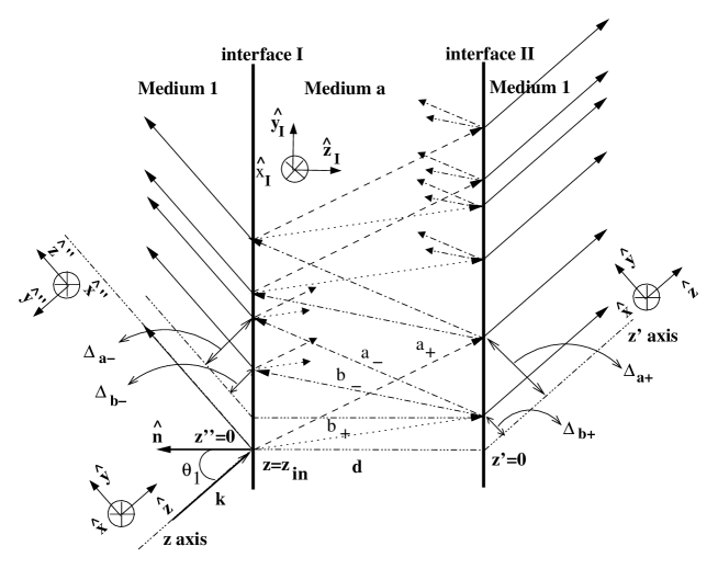
Fig. 1: Schematic view of the plane wave propagation in the anisotropic slab. For the sake of clarity, some of the inner reflected rays are represented by small arrows. The plane of incidence coincides with the plane $yz$. Symbols $a_{\pm}$ and $b_{\pm}$ correspond to the four possible propagation directions for the incident angle $\theta_{1}$. The four elementary transverse walk-offs, $\Delta_{a_{\pm}}$ and $\Delta_{b_{\pm}}$, are indicated. The different vector basis used throughout this article are also shown: $\{\mbox{${\rm\bf\hat{x}}$ },\mbox{${\rm\bf\hat{y}}$ },\mbox{${\rm\bf\hat{z}}$ }\}$ for the incidesfigure4nt and transmitted beams, $\{\mbox{${\rm\bf\hat{x}}$ }^{\prime\prime},\mbox{${\rm\bf\hat{y}}$ }^{\prime\prime},\mbox{${\rm\bf\hat{z}}$ }^{\prime\prime}\}$ for the reflected beam, $\{\mbox{${\rm\bf\hat{x}_{I}}$ },\mbox{${\rm\bf\hat{y}_{I}}$ },\mbox{${\rm\bf\hat{z}_{I}}$ }\}$ to perform calculations of the birefringence effects. Attached to the two former bases are the axis of propagation: $z$ axis for the incident beam, $z^{\prime}$ axes for the transmitted beam and $z^{\prime\prime}$ axis for the reflected beam.

In the paraxial approximation, an electromagnetic scalar field amplitude $\psi(\mbox{ ${\rm\bf r_{\perp}}$},z=0)$ can be expanded according to

$$\psi(\mbox{ ${\rm\bf r_{\perp}}$},0)={\cal F}[{\overline{\psi}}(\mbox{$\rm\bf k_{\perp}$})]=\frac{\displaystyle 1}{\displaystyle 2\pi}\iint{\overline{\psi}}(\mbox{$\rm\bf k_{\perp}$})\exp(-i\mbox{$\rm\bf k_{\perp}$}\cdot\mbox{ ${\rm\bf r}$})d^{2}\mbox{$\rm\bf k_{\perp}$}$$ (1)

where the time dependence has been omitted and where $\mbox{$\rm\bf k_{\perp}$}=k_{x}\mbox{${\rm\bf\hat{x}}$ }+k_{y}\mbox{${\rm\bf\hat{y}}$ }$ and $|\mbox{$\rm\bf k_{\perp}$}|\ll k$ so that $k_{z}\approx k(1-|\mbox{$\rm\bf k_{\perp}$}|^{2}/(2k^{2}))$. In Eq. (1), ${\overline{\psi}}(\mbox{$\rm\bf k_{\perp}$})$ is the scalar field amplitude in the $\rm\bf k_{\perp}$ space. To satisfy the paraxial approximation, ${\overline{\psi}}(\mbox{$\rm\bf k_{\perp}$})$ must be such that the integral has appreciable values only for $|\mbox{$\rm\bf k_{\perp}$}|\ll k$.

At a given plane $z\neq 0$, the field is given by ${}^{\hbox{\immediate{\bf{?}}}}$

$$\psi(\mbox{ ${\rm\bf r_{\perp}}$},z)=\exp\biggl{(}\frac{\displaystyle-iz}{\displaystyle 2k}(P_{x}^{2}+P_{y}^{2})\biggr{)}\psi(\mbox{ ${\rm\bf r_{\perp}}$},0)$$ (2)

where, as all along this article, the term $\exp(ikz)$ has been omitted and where

$$P_{x}=-i\frac{\partial}{\partial x},\,\,P_{y}=-i\frac{\partial}{\partial y}.$$

Eq. (1) can then be written

$$\psi(\mbox{ ${\rm\bf r_{\perp}}$},z)={\cal F}[{\overline{\psi}}(\mbox{$\rm\bf k_{\perp}$},z)],$$

where we define for convenience

$${\overline{\psi}}(\mbox{$\rm\bf k_{\perp}$},z)={\overline{\psi}}(\mbox{$\rm\bf k_{\perp}$})\exp\biggl{(}\frac{\displaystyle iz}{\displaystyle 2k}\mbox{$\rm\bf k^{2}_{\perp}$}\biggr{)}.$$

For a paraxial Gaussian beam, it is easy to show that

$$\psi(\mbox{ ${\rm\bf r_{\perp}}$},0)=\sqrt{\frac{2}{\pi w_{0}^{2}}}\exp\biggl{(}\frac{\displaystyle-\mbox{ ${\rm\bf r^{2}_{\perp}}$}}{\displaystyle w_{0}^{2}}\biggr{)}\Longrightarrow\begin{cases}\psi(\mbox{ ${\rm\bf r_{\perp}}$},z)=\sqrt{\frac{2}{\pi w_{0}^{2}}}\frac{\displaystyle-iz_{R}}{\displaystyle q(z)}\exp\biggl{(}\frac{\displaystyle-ik\mbox{ ${\rm\bf r^{2}_{\perp}}$}}{\displaystyle 2q(z)}\biggr{)}\\ {\overline{\psi}}(\mbox{$\rm\bf k_{\perp}$},z)=\frac{w_{0}}{\sqrt{2\pi}}\exp\biggl{(}\frac{\displaystyle iq(z)\mbox{$\rm\bf k^{2}_{\perp}$}}{\displaystyle 2k}\biggr{)}\end{cases}$$

where $w_{0}$ is the beam waist, $q(z)=z+iz_{R}$ is the complex radius of curvature and $z_{R}=kw_{0}^{2}$ is the Rayleigh range.

Eq. (1) is the plane wave expansion of the vector Gaussian beam. Wave vectors of these plane waves are defined by

$${\rm\bf k_{pw}}=\mbox{$\rm\bf k_{\perp}$}+k_{z}\mbox{${\rm\bf\hat{z}}$ }\approx\mbox{$\rm\bf k_{\perp}$}+k(1-\frac{\displaystyle|\mbox{$\rm\bf k_{\perp}$}|^{2}}{\displaystyle 2k^{2}})\mbox{${\rm\bf\hat{z}}$ }$$ (3)

in the paraxial approximation. However, Eq. (1) does not take into account the vectorial nature of the electromagnetic field. To keep the orthogonality between the electric field, magnetic field and wave vector of each plane waves, one must introduce the six component vector ${}^{\hbox{\immediate{?}}}$

$$F(\mbox{ ${\rm\bf r_{\perp}}$},0)=\begin{pmatrix}E_{x}(\mbox{ ${\rm\bf r_{\perp}}$},0)\\ E_{y}(\mbox{ ${\rm\bf r_{\perp}}$},0)\\ E_{z}(\mbox{ ${\rm\bf r_{\perp}}$},0)\\ B_{x}(\mbox{ ${\rm\bf r_{\perp}}$},0)\\ B_{y}(\mbox{ ${\rm\bf r_{\perp}}$},0)\\ B_{z}(\mbox{ ${\rm\bf r_{\perp}}$},0)\end{pmatrix}$$

and use the following Fourier transformation ${}^{\hbox{\immediate{?}}}$

$$F(\mbox{ ${\rm\bf r_{\perp}}$},0)=\frac{1}{2\pi}\iint{\overline{\psi}}(\mbox{$\rm\bf k_{\perp}$})\exp(-i\mbox{$\rm\bf k_{\perp}$}\cdot\mbox{ ${\rm\bf r_{\perp}}$})\exp\biggl{(}i\frac{\displaystyle k_{x}}{\displaystyle k}G_{x}+i\frac{\displaystyle k_{y}}{\displaystyle k}G_{y}\biggr{)}\begin{pmatrix}a_{1}\\ a_{2}\\ 0\\ -a_{2}\\ a_{1}\\ 0\end{pmatrix}d^{2}\mbox{$\rm\bf k_{\perp}$}$$ (4)

where $G_{x}$ and $G_{y}$ are $6\times 6$ matrices which are derived from the Poincaré group algebra .${}^{\hbox{\immediate{?}}}$ Expressions of these matrices can be found in Ref. ?. It should be noticed that the orthogonality between the electric field, magnetic field and wave vector of the plane waves only holds in the paraxial approximation, i.e. up to the order ${\cal O}(|\mbox{$\rm\bf k_{\perp}$}|^{2}/k^{2})$.

Expression of $F(\mbox{ ${\rm\bf r_{\perp}}$},z)$ is obtained similarly to Eq. (2)

$$F(\mbox{ ${\rm\bf r_{\perp}}$},z)=\frac{1}{2\pi}\iint{\overline{\psi}}(\mbox{$\rm\bf k_{\perp}$},z)\exp(-i\mbox{$\rm\bf k_{\perp}$}\cdot\mbox{ ${\rm\bf r_{\perp}}$})M_{6\times 6}\begin{pmatrix}a_{1}\\ a_{2}\\ 0\\ -a_{2}\\ a_{1}\\ 0\end{pmatrix}d^{2}\mbox{$\rm\bf k_{\perp}$},$$ (5)

with

$$M_{6\times 6}=\left(\begin{array}[]{cccccc}1+{\frac{{{k_{y}^{2}}}-{{k_{x}^{2}}}}{8{k}^{2}}}&{\frac{{-k_{y}}{k_{x}}}{4{k}^{2}}}&{\frac{{k_{x}}}{2k}}&{\frac{{k_{y}}{k_{x}}}{4{k}^{2}}}&{\frac{{{k_{y}^{2}}}-{{k_{x}^{2}}}}{8{k}^{2}}}&{\frac{{-k_{y}}}{2k}}\\ \vskip 6.0pt plus 2.0pt minus 2.0pt\cr{\frac{-{k_{y}}{k_{x}}}{4{k}^{2}}}&{1-\frac{{{k_{y}^{2}}}-{{k_{x}^{2}}}}{8{k}^{2}}}&{\frac{{k_{y}}}{2k}}&{\frac{{{k_{y}^{2}}}-{{k_{x}}}^{2}}{8{k}^{2}}}&{\frac{-{k_{y}}{k_{x}}}{4{k}^{2}}}&{\frac{{k_{x}}}{2k}}\\ \vskip 6.0pt plus 2.0pt minus 2.0pt\cr{\frac{{-k_{x}}}{2k}}&{\frac{{-k_{y}}}{2k}}&1&{\frac{{k_{y}}}{2k}}&{\frac{{-k_{x}}}{2k}}&0\\ \vskip 6.0pt plus 2.0pt minus 2.0pt\cr{\frac{{-k_{y}}{k_{x}}}{4{k}^{2}}}&{\frac{-{{k_{y}^{2}}}+{{k_{x}^{2}}}}{8{k}^{2}}}&{\frac{{k_{y}}}{2k}}&1+{\frac{{{k_{y}^{2}}}-{{k_{x}}}^{2}}{8{k}^{2}}}&{\frac{{-k_{y}}{k_{x}}}{4{k}^{2}}}&{\frac{{k_{x}}}{2k}}\\ \vskip 6.0pt plus 2.0pt minus 2.0pt\cr{\frac{-{{k_{y}^{2}}}+{{k_{x}^{2}}}}{8{k}^{2}}}&{\frac{{k_{y}}{k_{x}}}{4{k}^{2}}}&{\frac{{-k_{x}}}{2k}}&{\frac{-{k_{y}}{k_{x}}}{4{k}^{2}}}&1-{\frac{{{k_{y}^{2}}}-{{k_{x}^{2}}}}{8{k}^{2}}}&{\frac{{k_{y}}}{2k}}\\ \vskip 6.0pt plus 2.0pt minus 2.0pt\cr{\frac{{-k_{y}}}{2k}}&{\frac{{k_{x}}}{2k}}&0&{\frac{{-k_{x}}}{2k}}&{\frac{{-k_{y}}}{2k}}&1\end{array}\right).$$

Focusing on the electric field, Eq. (5) can be reduced to a $3\times 3$ matrix equation

$$\begin{pmatrix}E_{x}(\mbox{ ${\rm\bf r}$})\\ E_{y}(\mbox{ ${\rm\bf r}$})\\ E_{z}(\mbox{ ${\rm\bf r}$})\end{pmatrix} = {\cal F}[{\overline{\psi}}(\mbox{$\rm\bf k_{\perp}$},z)M_{3\times 3}\mbox{${\rm\bf E_{0}}$}]$$

$$= \frac{1}{2\pi}\iint{\overline{\psi}}(\mbox{$\rm\bf k_{\perp}$},z)\exp(-i\mbox{$\rm\bf k_{\perp}$}\cdot\mbox{ ${\rm\bf r_{\perp}}$})M_{3\times 3}\mbox{${\rm\bf E_{0}}$}d^{2}\mbox{$\rm\bf k_{\perp}$}$$

with $\mbox{${\rm\bf E_{0}}$}^{T}=(a_{1},a_{2},0)$ and

$$M_{3\times 3}=\begin{pmatrix}1+{\frac{{{k_{y}^{2}}}-{{k_{x}^{2}}}}{4{k}^{2}}}&{\frac{{-k_{y}}{k_{x}}}{2{k}^{2}}}&0\\ {\frac{{-k_{y}}{k_{x}}}{2{k}^{2}}}&1-{\frac{{{k_{y}^{2}}}-{{k_{x}^{2}}}}{4{k}^{2}}}&0\\ {\frac{{-k_{x}}}{k}}&{\frac{{-k_{y}}}{k}}&0\\ \end{pmatrix}.$$ (7)

Notices that the same expression holds for the magnetic field.

One can verify that, for an electric vector polarized along ${\rm\bf\hat{x}}$ (i.e. $\mbox{${\rm\bf E_{0}}$}^{T}=(1,0,0)$), the integration of Eq. (2) over $\rm\bf k_{\perp}$ leads to the results of Ref. ?. The angular divergence of a Gaussian beam therefore generates crossed polarization effects.

3 Application to anisotropic layer

We shall now consider a Gaussian beam crossing a single anisotropic parallel plate of thickness $d$ surrounded by a dielectric medium of optical index $N_{1}$. The plate is located at $z=z_{in}$ and tilted with respect to ${\rm\bf k}$ (see Fig. 1). The optical axis has an a priori arbitrary orientation. To compute the transmitted beam, the vector Fourier optics and the $4\times 4$ matrix formalism of Ref. ? will be combined. In doing so, multiple reflections inside the parallel plate will be taken into account.

As indicated in Ref. ?, polarization effects induced by the anisotropic plate can be computed by defining an operator acting on every plane waves constituting the Gaussian beam. This is further justified since we do only consider here homogeneous anisotropic media. Hence, writing ${\rm\bf E}_{t}(\mbox{ ${\rm\bf r}$})$ for the transmitted beam, one obtains ${}^{\hbox{\immediate{?},\penalty 1000\hskip 0.91003pt plus 0.70004pt minus 0.70004pt{\bf{?}}}}$

$${\rm\bf E}_{t}(\mbox{ ${\rm\bf r}$}^{\prime})=\exp\biggl{(}\frac{-iz^{\prime}}{2k}(P_{x}^{2}+P_{y}^{2})\biggr{)}{\cal F}\biggl{[}{\overline{M}}_{t}\exp\biggl{(}\frac{-iz_{in}}{2k}(P_{x}^{2}+P_{y}^{2})\biggr{)}{\overline{\psi}}(\mbox{$\rm\bf k_{\perp}$},0)M_{3\times 3}\mbox{${\rm\bf E_{0}}$}\biggr{]}.$$ (8)

In Eq. (8), ${\overline{M}}_{t}$ is a $3\times 3$ matrix acting on the polarization state of each plane wave and $z^{\prime}$ is an axis parallel to the $z$ axis with $z^{\prime}=0$ at the exit of the plate (see Fig. 1). This axis is used to describe the beam propagation after the plate. Inside the plate, the propagation of the plane waves is described by the matrix ${\overline{M}}_{t}$. Let us mention that the position of the $z^{\prime}$ axis along the exit face of the plate can be arbitrarily chosen since it only introduces a global phase shift.

However, in Eq. (8) ${\overline{M}}_{t}$ is determined in the basis $\{\mbox{${\rm\bf\hat{x}}$ },\mbox{${\rm\bf\hat{y}}$ },\mbox{${\rm\bf\hat{z}}$ }\}$. For consistency with the general $4\times 4$ matrix method ,${}^{\hbox{\immediate{?}}}$ ${\overline{M}}_{t}$ must be determined in the plane wave polarization basis. The polarization vector basis is denoted by $\{\mbox{${\rm\bf\hat{s}_{pw}}$},\mbox{${\rm\bf\hat{p}_{pw}}$},\mbox{${\rm\bf\hat{k}_{pw}}$}\}$ where

$$\mbox{${\rm\bf\hat{s}_{pw}}$}=\frac{\mbox{${\rm\bf\hat{k}_{pw}}$}\times{\rm\bf\hat{n}}}{|\mbox{${\rm\bf\hat{k}_{pw}}$}\times{\rm\bf\hat{n}}|},\,\,\,\mbox{${\rm\bf\hat{p}_{pw}}$}=\mbox{${\rm\bf\hat{k}_{pw}}$}\times\mbox{${\rm\bf\hat{s}_{pw}}$}$$

correspond to the TE and TM waves respectively and where ${\rm\bf\hat{n}}$ is the unit vector normal to the interface. The direction of the wave vector reads $\mbox{${\rm\bf\hat{k}_{pw}}$}={\rm\bf k_{pw}}/k$ with ${\rm\bf k_{pw}}$ given by Eq. (3) and by convention, $\{\mbox{${\rm\bf\hat{s}_{pw}}$},\mbox{${\rm\bf\hat{p}_{pw}}$},\mbox{${\rm\bf\hat{k}_{pw}}$}\}=\{\mbox{${\rm\bf\hat{x}}$ },\mbox{${\rm\bf\hat{y}}$ },\mbox{${\rm\bf\hat{z}}$ }\}$ when $\mbox{$\rm\bf k_{\perp}$}=0$.

The plane of incidence being related to the plane wave vector one gets

$${\overline{M}}_{t}=\Omega M_{t}\Omega^{T}$$ (9)

with

$$\Omega = \begin{pmatrix}\mbox{${\rm\bf\hat{x}}$ }\cdot\mbox{${\rm\bf\hat{s}_{pw}}$}&\mbox{${\rm\bf\hat{x}}$ }\cdot\mbox{${\rm\bf\hat{p}_{pw}}$}&\mbox{${\rm\bf\hat{x}}$ }\cdot\mbox{${\rm\bf\hat{k}_{pw}}$}\\ \mbox{${\rm\bf\hat{y}}$ }\cdot\mbox{${\rm\bf\hat{s}_{pw}}$}&\mbox{${\rm\bf\hat{y}}$ }\cdot\mbox{${\rm\bf\hat{p}_{pw}}$}&\mbox{${\rm\bf\hat{y}}$ }\cdot\mbox{${\rm\bf\hat{k}_{pw}}$}\\ \mbox{${\rm\bf\hat{z}}$ }\cdot\mbox{${\rm\bf\hat{s}_{pw}}$}&\mbox{${\rm\bf\hat{z}}$ }\cdot\mbox{${\rm\bf\hat{p}_{pw}}$}&\mbox{${\rm\bf\hat{z}}$ }\cdot\mbox{${\rm\bf\hat{k}_{pw}}$}\end{pmatrix},$$ (10)

$$M_{t} = \left(\begin{array}[]{c c}{\cal M}_{t}&\begin{array}[]{c}0\\ 0\end{array}\\ \begin{array}[]{c c}0&0\end{array}&0\\ \end{array}\right)$$ (16)

and where ${\cal M}_{t}$ is the $2\times 2$ matrix describing the transmission of the plane waves in the $\{\mbox{${\rm\bf\hat{s}_{pw}}$},\mbox{${\rm\bf\hat{p}_{pw}}$}\}$ basis. The matrix ${\cal M}_{t}$ is obtained by reducing the $4\times 4$ matrix method of Ref. ? to a $2\times 2$ matrix algebra as described in the following section.

A $2\times 2$ matrix algebra for plane wave propagation inside anisotropic parallel plates

Because of linearity, the relations between incident, reflected and refracted plane waves amplitudes at an interface between two anisotropic media can be written in a $2\times 2$ matrix form. For the two interfaces I and II of the single layer of Fig. 1, we thus introduce the following $2\times 2$ matrices:

$$\mbox{Reflection $1\rightarrow a$ at interface I }: \,{\cal R}_{1a_{+}}$$ (17)

$$\mbox{Transmission $1\rightarrow a$ at interface I }: \,{\cal P}_{+}^{-1}{\cal T}_{1a_{+}}$$ (18)

$$\mbox{Reflection $a\rightarrow 1$ at interface I }: \,{\cal P}^{-1}_{+}{\cal R}_{a1_{-}}{\cal P}_{-}$$ (19)

$$\mbox{Transmission $a\rightarrow 1$ at interface I }: \,{\cal T}_{a1_{-}}{\cal P}_{-}$$ (20)

$$\mbox{Reflection $a\rightarrow 1$ at interface II }: \,{\cal R}_{a1_{+}}$$ (21)

$$\mbox{Transmission $a\rightarrow 1$ at interface II }: \,{\cal T}_{a1_{+}}$$ (22)

where the $+$ and $-$ subscripts refer to forward and backward beam propagations respectively. ${\cal R}$ and ${\cal T}$ matrices describe the reflection and transmission of the plane waves. ${\cal P}_{\pm}$ are the diagonal phase shift matrices

$${\cal P}_{\pm}=\begin{pmatrix}\exp(id{\rm\bf k}_{a_{\pm}}\cdot{\rm\bf\hat{n}})&0\\ 0&\exp(id{\rm\bf k}_{b_{\pm}}\cdot{\rm\bf\hat{n}})\\ \end{pmatrix}$$

where ${\rm\bf k}_{a_{\pm}}$ and ${\rm\bf k}_{b_{\pm}}$ are the four possible wave vectors ,${}^{\hbox{\immediate{?}}}$ inside the anisotropic medium, corresponding to the incident wave vector defined in Eq. (3). In the above expression, ${\rm\bf\hat{n}}$ is the unit vector normal to the interface.

All the matrices of Eqs. (17-22) are different in the general case of a biaxial medium. They are determined by the electromagnetic field continuity conditions at interfaces I and II of Fig. 1 according to the method of Ref. .${}^{\hbox{\immediate{?}}}$

Writing ${\bf E}_{pw,i}$ and ${\bf E}_{pw,t}$ the electric field vectors for an incident plane wave at interface I and the transmitted plane wave at interface II, we obtain

$${\bf E}_{pw,t}=\biggl{(}{\cal T}_{a1_{+}}{{\cal P}}_{+}^{-1}{\cal T}_{1a_{+}}+{\cal T}_{a_{+}}{{\cal P}}_{+}^{-1}{\cal R}_{a1_{-}}{{\cal P}}_{-}{\cal R}_{a1_{+}}{{\cal P}}_{+}^{-1}{\cal T}_{1a_{+}}+\cdots\biggr{)}{\bf E}_{pw,i},$$

using Eqs. (17-22). This expression can be simplified utilising $\sum_{j=0}^{\infty}X^{j}=(1-X)^{-1}$:

$${\cal M}_{t}={\cal T}_{a1_{+}}\biggl{[}1-{\cal P}^{-1}_{+}{\cal R}_{a1_{-}}{\cal P}_{-}{\cal R}_{a1_{+}}\biggr{]}^{-1}{\cal P}^{-1}{\cal T}_{1a_{+}},$$ (23)

with ${\bf E}_{pw,t}={\cal M}_{t}{\bf E}_{pw,i}$.

Let us mention that using the same procedure one can also determine the reflected electric vector at the interface I of Fig. 1.

B Transmitted beam Intensity

Turning back to the transmission of Gaussian beams, Eq. (8) can be further simplified when one is interested by intensity measurements. For example, if an optical polarization component is located upward the anisotropic medium, the out-coming electric field reads

$${\bf E}_{out}(\mbox{ ${\rm\bf r}$})=\frac{w_{0}}{\sqrt{2\pi}}{\cal F}\biggl{[}\exp\biggl{(}i\frac{(z_{in}+z^{\prime})\mbox{$\rm\bf k^{2}_{\perp}$}}{k}\biggr{)}\exp\biggl{(}\frac{-w_{0}^{2}\mbox{$\rm\bf k^{2}_{\perp}$}}{4}\biggr{)}J{\overline{M}}_{t}M_{3\times 3}\mbox{${\rm\bf E_{0}}$}\biggr{]}$$

where

$$J=\left(\begin{array}[]{c c}{\cal J}&\begin{array}[]{c}0\\ 0\end{array}\\ \begin{array}[]{c c}0&0\end{array}&0\\ \end{array}\right)$$

and ${\cal J}$ is the $2\times 2$ Jones matrix corresponding to this component .${}^{\hbox{\immediate{?}}}$ The total intensity measured after this component is given by

$$I_{out} = \iint|{\rm\bf E}_{out}|^{2}d^{2}\mbox{ ${\rm\bf r_{\perp}}$}$$ (24)

$$= \frac{w_{0}^{2}}{(2\pi)^{3}}\idotsint\exp\biggl{(}\frac{-w_{0}^{2}(\mbox{$\rm\bf k^{2}_{\perp}$}+\mbox{$\rm\bf k^{{}^{\prime}2}_{\perp}$})}{4}\biggr{)}\exp\biggl{(}i\frac{(z_{in}+z^{\prime})(\mbox{$\rm\bf k^{2}_{\perp}$}+\mbox{$\rm\bf k^{{}^{\prime}2}_{\perp}$})}{k}\biggr{)}$$

$$\biggr{[}O_{3\times 3}\mbox{${\rm\bf E_{0}}$}\biggl{]}\cdot\biggl{[}O^{*}_{3\times 3}(\mbox{$\rm\bf k^{\prime}_{\perp}$})\mbox{${\rm\bf E_{0}}$}^{*}\biggr{]}\exp(i(\mbox{$\rm\bf k_{\perp}$}-\mbox{$\rm\bf k^{\prime}_{\perp}$})\cdot\mbox{ ${\rm\bf r_{\perp}}$})d^{2}\mbox{$\rm\bf k_{\perp}$}d^{2}\mbox{$\rm\bf k^{\prime}_{\perp}$}d^{2}\mbox{ ${\rm\bf r_{\perp}}$}$$

with $O_{3\times 3}={J}{\overline{M}}_{t}M_{3\times 3}$ and where the symbol * stands for the complex conjugate.

If the matrix ${J}$ does not depend on the transverse spatial coordinates, the previous equation is simplified

$$I_{out}=\frac{w_{0}^{2}}{2\pi}\iint\exp\biggl{(}\frac{-w_{0}^{2}\mbox{$\rm\bf k^{2}_{\perp}$}}{2}\biggr{)}\biggr{|}O_{3\times 3}\mbox{${\rm\bf E_{0}}$}\biggr{|}^{2}d^{2}\mbox{$\rm\bf k_{\perp}$}$$ (25)

after integrations over ${\rm\bf r_{\perp}}$ and $\rm\bf k^{\prime}_{\perp}$ and using

$$\delta^{2}(\mbox{$\rm\bf k_{\perp}$}-\mbox{$\rm\bf k^{\prime}_{\perp}$})=(2\pi)^{2}\iint\exp(i(\mbox{$\rm\bf k_{\perp}$}-\mbox{$\rm\bf k^{\prime}_{\perp}$})\cdot\mbox{ ${\rm\bf r_{\perp}}$})d^{2}\mbox{ ${\rm\bf r_{\perp}}$}$$

where $\delta^{2}(\mbox{$\rm\bf k_{\perp}$}-\mbox{$\rm\bf k^{\prime}_{\perp}$})$ is the Dirac distribution.

Eq. (25) shows explicitly that the total intensity depends only on the waist and not on the beam size inside the anisotropic system. This observation has been already made and experimentally tested in Ref. ?.

Up to now only the transmission has been considered. Equivalent expressions can be obtained for the reflection by simply replacing ${\cal M}_{t}$ by the extended Jones matrix describing the reflection.

Eq. (25) was obtained under the paraxial approximation. This equation can be used as it is but, depending on the required accuracy, one can perform further simplifications: the plane wave approximation and the Scalar Fourier approximation. The latter is the topic of the following section.

4 Scalar Fourier Approximation

Although the vector Fourier optics is a useful formalism to describe the Gaussian beam, the cross polarization effects are indeed very small ${}^{\hbox{\immediate{?}}}$ (though being observable but essentially in extinction experiments${}^{\hbox{\immediate{?}}}$). In addition, the birefringence induced by the beam angular divergence is also expected to be small, at least for realistic ellipsometry experiments.

To a good approximation, one can then assume that all plane waves constituting the Gaussian beam have the same wave vector ${\rm\bf k}$ (i.e. $\mbox{$\rm\bf k_{\perp}$}=0$). The polarization effects induced by a birefringent plate will then be only related to the direction of the Gaussian beam’s center.

This approximation thus amounts to account for the Gaussian nature of the beam only in the calculation of the interference pattern of the beam after the plate, as in Ref. ?. After the anisotropic plate, the beam is made of a sum of Gaussian beams transversally shifted by a distance (the transverse walk-off), induced by successive internal reflections (see Fig. 1). Using Eqs. (17-22), the first transmitted beam can be written

$${\rm\bf E}_{1t}(\mbox{ ${\rm\bf r}$}^{\prime})= \biggl{(}{\frac{2}{\pi\omega_{0}^{2}}}\biggr{)}^{1/2}\frac{-iz_{R}}{q(z^{\prime}+z_{in})}\exp\biggl{(}\frac{-ikx^{{}^{\prime}2}}{2q(z^{\prime}+z_{in})}\biggr{)}\biggl{[}$$

$${\cal T}_{a1_{+}}\begin{pmatrix}\exp\biggl{(}\frac{-ik(y^{\prime}-\Delta_{a_{+}})^{2}}{2q(z^{\prime}+z_{in})}\biggr{)}&0\\ 0&\exp\biggl{(}\frac{-ik(y^{\prime}-\Delta_{b_{+}})^{2}}{2q(z^{\prime}+z_{in})}\biggr{)}\\ \end{pmatrix}{\cal P}_{+}^{-1}{\cal T}_{1a_{+}}\biggr{]}\mbox{${\rm\bf e_{0}}$}$$ (26)

with $\mbox{${\rm\bf e_{0}}$}^{T}=(a_{1},a_{2})$ and where $\Delta_{a_{+}}$ and $\Delta_{b_{+}}$ are the transverse walk-offs. In biaxial media there are four different elementary transverse walk-offs

$${\Delta}_{a_{\pm}}=\frac{c}{\omega}\frac{N_{1}d\sin\theta_{1}\cos\theta_{1}}{|{\overline{\rm\bf k}}_{a_{\pm}}\cdot{\rm\bf\hat{n}}|},\,\,{\Delta}_{b_{\pm}}=\frac{c}{\omega}\frac{N_{1}d\sin\theta_{1}\cos{\theta_{1}}}{|{\overline{\rm\bf k}}_{b_{\pm}}\cdot{\rm\bf\hat{n}}|},$$

where ${\overline{\rm\bf k}}_{a_{\pm}}$ and ${\overline{\rm\bf k}}_{b_{\pm}}$ are the wave vectors inside the anisotropic plate corresponding to the incident wave vector ${\rm\bf k}$, i.e. the center of the Gaussian beam. We should specify that all the matrices of Eqs. (17-22) are also determined with respect to the direction of the center of the Gaussian beam.

When the transmission and reflection interface matrices are not diagonal it becomes difficult, if not impossible, to write a general formula for the $n^{th}$ transmitted beam. However, using the following property of the Fourier transform

$$\psi(\mbox{ ${\rm\bf r_{\perp}}$},z)={\cal F}[{\overline{\psi}}(\mbox{$\rm\bf k_{\perp}$},z)]\Rightarrow\psi(\mbox{ ${\rm\bf r_{\perp}}$}-\Delta\mbox{${\rm\bf\hat{y}}$ },z)={\cal F}[{\overline{\psi}}(\mbox{$\rm\bf k_{\perp}$},z)\exp(i\Delta k_{y})],$$ (27)

and taking the inverse Fourier transform of Eq. (26), one obtains

$${\cal F}^{-1}[{\rm\bf E}_{1t}(\mbox{ ${\rm\bf r}$}^{\prime})]= \biggl{(}\frac{w_{0}^{2}}{2\pi}\biggr{)}^{1/2}\exp\biggl{(}i\frac{(z_{in}+z^{\prime})\mbox{$\rm\bf k^{2}_{\perp}$}}{k}\biggr{)}\exp\biggl{(}\frac{-w_{0}^{2}\mbox{$\rm\bf k^{2}_{\perp}$}}{4}\biggr{)}\biggl{[}$$

$${\cal T}_{a1_{+}}\begin{pmatrix}\exp(ik_{y}\Delta_{a_{+}})&0\\ 0&\exp(ik_{y}\Delta_{b_{+}})\\ \end{pmatrix}{\cal P}_{+}^{-1}{\cal T}_{1a_{+}}\biggr{]}\mbox{${\rm\bf e_{0}}$}.$$

It is therefore possible to sum up all the transmitted beams in the $\rm\bf k_{\perp}$ space by introducing a new set of $2\times 2$ matrices:

$${\cal W}_{\pm}=\begin{pmatrix}\exp(i{\Delta}_{a_{\pm}}k_{y})&0\\ 0&\exp(i{\Delta}_{b_{\pm}}k_{y})\end{pmatrix}$$ (28)

describing the transverse walk-off of the Gaussian beam’s center (see Fig. 1).
Following the method introduced in the previous section, one then obtains

$${\rm\bf E}_{t}(\mbox{ ${\rm\bf r}$}^{\prime}) = \biggl{(}\frac{w_{0}^{2}}{2\pi}\biggr{)}^{1/2}{\cal F}\biggl{[}\exp\biggl{(}i\frac{(z_{in}+z^{\prime})\mbox{$\rm\bf k^{2}_{\perp}$}}{k}\biggr{)}\exp\biggl{(}\frac{-w_{0}^{2}\mbox{$\rm\bf k^{2}_{\perp}$}}{4}\biggr{)}\biggl{(}{\cal T}_{a1_{+}}\widetilde{{\cal P}}_{+}^{-1}{\cal T}_{1a_{+}}+$$ (29)

$${\cal T}_{a_{+}}\widetilde{{\cal P}}_{+}^{-1}{\cal R}_{a1_{-}}\widetilde{{\cal P}}_{-}{\cal R}_{a1_{+}}\widetilde{{\cal P}}_{+}^{-1}{\cal T}_{1a_{+}}+\cdots\biggr{)}\mbox{${\rm\bf e_{0}}$}\biggr{]}$$

$$= \biggl{(}\frac{w_{0}^{2}}{2\pi}\biggr{)}^{1/2}{\cal F}\biggl{[}\exp\biggl{(}i\frac{(z_{in}+z^{\prime})k_{y}^{2}}{k}\biggr{)}\exp\biggl{(}\frac{-w_{0}^{2}k_{y}^{2}}{4}\biggr{)}\widetilde{{\cal M}}_{t}\mbox{${\rm\bf e_{0}}$}\biggr{]},$$

with

$$\widetilde{{\cal P}}_{+}^{-1} = {\cal W}_{+}{\cal P}_{+}^{-1}$$ (30)

$$\widetilde{{\cal P}}_{-} = {\cal W}_{-}{\cal P}_{-}$$ (31)

$$\widetilde{{\cal M}}_{t} = {\cal T}_{a1_{+}}\biggl{[}1-\widetilde{{\cal P}}^{-1}_{+}{\cal R}_{a1_{-}}\widetilde{{\cal P}}_{-}{\cal R}_{a1_{+}}\biggr{]}^{-1}\widetilde{{\cal P}}^{-1}_{+}{\cal T}_{1a_{+}}.$$ (32)

In the scalar Fourier approximation the usual Stokes vectors ${}^{\hbox{\immediate{\bf{?}}}}$ can be defined

$$S_{in}=\begin{pmatrix}|a_{1}|^{2}+|a_{2}|^{2}\\ |a_{1}|^{2}-|a_{2}|^{2}\\ a_{1}a_{2}^{*}+a_{1}^{*}a_{2}\\ i(a_{1}a_{2}^{*}-a_{1}^{*}a_{2})\end{pmatrix},\,\,S_{out}=\begin{pmatrix}\iint(|E_{tx}|^{2}+|E_{ty}|^{2})d^{2}\mbox{ ${\rm\bf r_{\perp}}$}\\ \iint(|E_{tx}|^{2}-|E_{ty}|^{2})d^{2}\mbox{ ${\rm\bf r_{\perp}}$}\\ \iint(E_{tx}E_{ty}^{*}+E_{tx}^{*}E_{ty})d^{2}\mbox{ ${\rm\bf r_{\perp}}$}\\ i\iint(E_{tx}E_{ty}^{*}-E_{tx}^{*}E_{ty})d^{2}\mbox{ ${\rm\bf r_{\perp}}$}\end{pmatrix},\,\,$$

where $S_{in}$ and $S_{out}$ are related to the incident beam and transmitted beam respectively. From Eq. (29) and following the calculation steps of section 3 one can then determine the extended Mueller matrix of the plate $M_{S}$ such $S_{out}=M_{S}S_{in}$:

$$M_{S}=\begin{pmatrix}(\rho^{2}_{11}+\rho^{2}_{12})/2+&(\rho^{2}_{11}+\rho^{2}_{21})/2-&\rho_{11,12}\cos\phi_{11,12}+&\rho_{11,12}\sin\phi_{11,12}+\\ (\rho^{2}_{21}+\rho^{2}_{22})/2&(\rho^{2}_{12}+\rho^{2}_{22})/2&\rho_{21,22}\cos\phi_{21,22}&\rho_{21,22}\sin\phi_{21,22}\\ &&&&\\ (\rho^{2}_{11}+\rho^{2}_{12})/2-&(\rho^{2}_{11}+\rho^{2}_{22})/2-&\rho_{11,12}\cos\phi_{11,12}-&\rho_{11,12}\sin\phi_{11,12}-\\ (\rho^{2}_{21}+\rho^{2}_{22})/2&(\rho^{2}_{21}+\rho^{2}_{12})/2&\rho_{21,22}\cos\phi_{21,22}&\rho_{21,22}\sin\phi_{21,22}\\ &&&&\\ \rho_{11,21}\cos\phi_{11,21}+&\rho_{11,21}\cos\phi_{11,21}-&\rho_{11,22}\cos\phi_{11,22}+&\rho_{11,22}\sin\phi_{11,22}-\\ \rho_{12,22}\cos\phi_{12,22}&\rho_{12,22}\cos\phi_{12,22}&\rho_{12,21}\cos\phi_{12,21}&\rho_{12,21}\sin\phi_{12,21}\\ &&&&\\ -\rho_{11,21}\sin\phi_{11,21}-&-\rho_{11,21}\sin\phi_{11,21}+&-\rho_{11,22}\sin\phi_{11,22}-&\rho_{11,22}\cos\phi_{11,22}-\\ \rho_{12,22}\sin\phi_{12,22}&\rho_{12,22}\sin\phi_{12,22}&\rho_{12,21}\sin\phi_{12,21}&\rho_{12,21}\cos\phi_{12,21}\\ \end{pmatrix}$$ (33)

with

$$\rho^{2}_{ij} = \frac{w_{0}}{\sqrt{2\pi}}\int\exp\biggl{(}\frac{-w_{0}^{2}k_{y}^{2}}{2}\biggr{)}|m_{ij}|^{2}dk_{y},$$ (34)

$$\rho_{ij,kl} = \frac{w_{0}}{\sqrt{2\pi}}\biggl{|}\int\exp\biggl{(}\frac{-w_{0}^{2}k_{y}^{2}}{2}\biggr{)}m_{ij}m^{*}_{kl}dk_{y}\biggr{|}$$

$$\cos\phi_{ij,kl} = \frac{1}{2\rho_{ij,kl}}\int\exp\biggl{(}\frac{-w_{0}^{2}k_{y}}{2}\biggr{)}[m_{ij}m^{*}_{kl}+m^{*}_{ij}m_{kl}]dk_{y}$$

$$\sin\phi_{ij,kl} = \frac{1}{2i\rho_{ij,kl}}\int\exp\biggl{(}\frac{-w_{0}^{2}k_{y}}{2}\biggr{)}[m_{ij}m^{*}_{kl}-m^{*}_{ij}m_{kl}]dk_{y}$$ (35)

and $i,j,k,l=1,2$. The matrix elements $m_{ij}$ are defined by

$${\cal J}\widetilde{{\cal M}}_{t}=\begin{pmatrix}m_{11}&m_{12}\\ m_{21}&m_{22}\end{pmatrix}.$$

One feature related to the integral form of Eqs. (34-35) is that $\rho_{ij,kl}\neq\rho_{ij}\rho_{kl}$. This means that one cannot define a Jones matrix (integrated over $\rm\bf k_{\perp}$).

5 Example: uniaxial parallel plate

To illustrate our model we shall now consider the very important example of a quarter wave Quartz plate (QWP) .${}^{\hbox{\immediate{\bf{?}}}}$ The equivalence between our approach and the results of Ref. ? is formally proved in Appendix I and details concerning the evaluation of Eq. (25) are given in Appendix II.

To study the accuracy of the plane wave and scalar Fourier approximations we shall adopt one of the examples of Ref. ?: a Gaussian laser beam of wavelength $\lambda=0.6328\,{\rm\mu m}$ and waist $w_{0}=100\,{\rm\mu m}$. For this wavelength, the Quartz ordinary and extraordinary optical indices are $n_{0}=1.542637$ and $n_{e}=1.551646$.

Since interference effects are sensitive to the plate thickness, we choose to compare two realistic components: a first order QWP ($d=87.6010\,{\rm\mu m}$) and a tenth order QWP ($d=719.9686\,{\rm\mu m}$). Finally, two different polar orientations of the optical axis (see Appendix II) are chosen $\theta_{c}=\pi/2$ (= optical axis in the plane of interface) and $\theta_{c}=\pi/4$. The remaining geometric degrees of freedom are the optical axis azimuth $\phi_{c}$ and the incidence angle of the center of the Gaussian beam $\theta_{1}$.

The incident beam is assumed to be polarized along $ox$ so that $\mbox{${\rm\bf E_{0}}$}=\mbox{${\rm\bf\hat{x}}$ }$ (or $S_{in}=(1,1,0,0)$). As in Fig. 1, the beam crosses a Quartz plate and we shall first consider that an intensity measurement is performed after a perfect linear polarizer aligned along $ox$. We shall denote $I_{||,Gauss}$ and $I_{||,pw}$ the corresponding intensities computed according to Eq. (33) (scalar Fourier approximation) and in the plane wave approximation. We checked numerically that results obtained in the scalar Fourier approximation agree with the general expression of 25 (to observe noticeable differences one must consider beam waits as small as $10\,{\rm\mu m}$ which are outside the scope of this article).

The relative numerical precision of the results presented below has been estimated to be of the order of $10^{-6}$. This number was determined by checking the energy conservation and by looking at the difference between the plane wave and the scalar Fourier approximation at normal incidence (they are similar by construction).

$I_{||,Gauss}$ is shown as function of $\phi_{c}$ and $\theta_{1}$ in Fig. 2(a-b) and 3(a-b) for the two plate thickness and the two orientations of the optical axis.

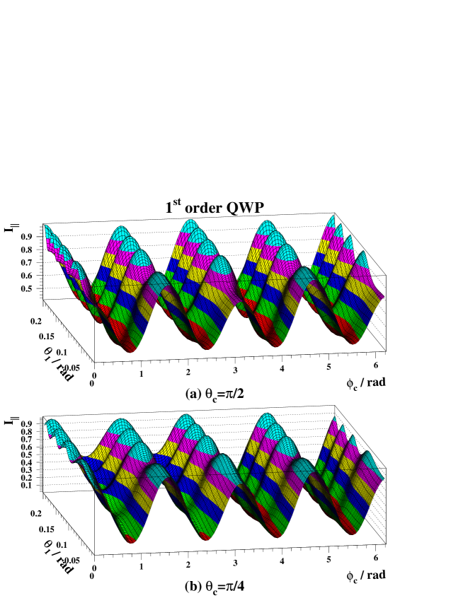
Fig. 2: Intensity of a Gaussian beam measured after a first order QWP and a perfect linear polarizer: (a) for an optical axis in the plane of interface, (b) for an optical axis inclined by $\pi/4$ with respect to the plane of interface. The calculations are performed using the scalar Fourier approximation and are shown as function of the angle of incidence $\theta_{1}$ and the azimuth angle of the optical axis $\phi_{c}$.

As expected ,${}^{\hbox{\immediate{?}}}$ the interference pattern is denser for the tenth order plate (Fig. 3(a) and (b)) and the intensity is not $\pi$ symmetric in $\phi_{c}$ when $\theta_{c}<\pi/2$ and $\theta_{1}\neq 0$ (Fig. 2(b) and 3(a)).

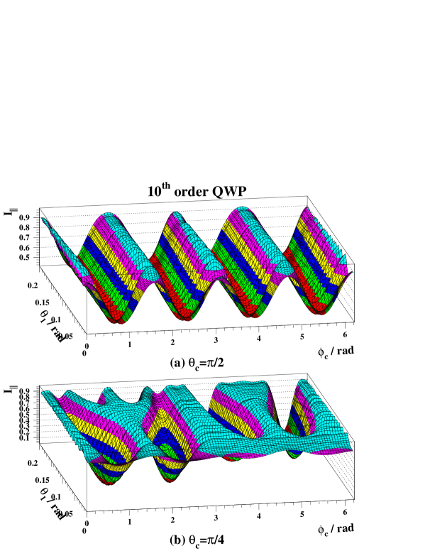
Fig. 3: Same as Fig.2 for a tenth order QWP.

Fixing $(\theta_{c}=\pi/2,\phi_{c}=0)$ and $(\theta_{c}=\pi/4,\phi_{c}=\phi/4)$, $I_{||,Gauss}$ and$I_{||,pw}$ are plotted as function of $\theta_{1}$ in Fig. 4 (a), (b) respectively for the tenth order QWP. In these figures, $I_{||,Gauss}$ is also computed for two beam waists $w_{0}=100\,{\rm\mu m}$ and $200\,{\rm\mu m}$. Sizable differences appear which increase with the incident angle but decrease when the beam waist increases.

To quantify the differences the following ratio is computed

$$\delta(I_{||})=\frac{I_{||,Gauss}-I_{||,pw}}{I_{||,Gauss}}$$

and plotted as function of $\phi_{c}$ and $\theta_{1}$ in Fig. Fig. 5(a-b) and 6(a-b) for the two plate thicknesses and the two orientations of the optical axis. One can sees that $\delta(I_{||})$ increases with the plate thickness and the angle of incidence. At $\theta_{1}\approx 0.2$ rad and $\theta_{c}=\pi/2$, large differences of the order of 10$\%$ appear for the tenth QWP. Variations of $\delta(I_{||})$ with $\phi_{c}$ are also sizable. Especially for $\theta_{c}<\pi/4$ where interference amplitudes are badly reproduced by the plane wave approximation for small values of $I_{||}$.

Fig. 4: Intensity of a Gaussian beam measured after a tenth order QWP and a perfect linear polarizer as function of the angle of incidence $\theta_{1}$. Orientations of the QWP optical axis are fixed to: (a) $\theta_{c}=\pi/2$ and $\phi_{c}=0$, (b) $\theta_{c}=\pi/4$ and $\phi_{c}=\pi/4$. Full lines and dashed lines represent the calculations performed using the scalar Fourier approximations for $w_{0}=100\,{\rm m\mu}$ and $w_{0}=200\,{\rm m\mu}$ respectively. Dotted lines show the calculations performed using the plane wave approximation.

Another interesting quantity is the degree of circular polarisation when the beam passes through a perfect circular polarizer, instead of the linear polarizer of the above example. If the polarizer is circular left, using Eq. (33) and the standard Mueller matrices for perfect polarizers ${}^{\hbox{\immediate{?}}}$ the beam intensity reads

$$I_{L}=\frac{\rho^{2}_{11}+\rho^{2}_{21}}{2}-\rho_{11,21}\sin\phi_{11,21}$$

for $S_{in}=(1,1,0,0)$ and $\theta_{c}=\pi/2$. When $\phi_{c}\approx\pi/4$, $I_{L}$ is small and can be minimized in the $(\theta_{1},\phi_{c})$ space .${}^{\hbox{\immediate{?}}}$ We present here $I_{L}^{-1}$ as function of $\theta_{1}$ and $\phi_{c}$ for the tenth order QWP in Fig. 7(a).
Results of Ref. ? are recovered although rotating the plate and rotating the polarization, as done in this reference, are not strictly equivalent .${}^{\hbox{\immediate{\bf{?}},\penalty 1000\hskip 0.91003pt plus 0.70004pt minus 0.70004pt{\bf{?}},\penalty 1000\hskip 0.91003pt plus 0.70004pt minus 0.70004pt{\bf{?}}}}$ In Fig. 7(b) the relative difference between plane wave and Gaussian beam intensities

$$\delta(I_{L})=\frac{I_{L,Gauss}-I_{L,pw}}{I_{L,Gauss}}$$

is shown. Large differences corresponding to small values of $I_{L}$ are observed. This demonstrate the necessity to account for the Gaussian nature of the beam in such particular, but important, cases. It is to mention that the scalar Fourier approximation and the general paraxial calculations are here also in perfect agreement.

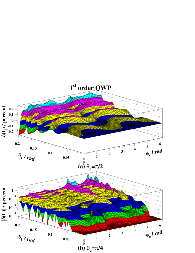
Fig. 5: Relative difference between the quantity of Fig.2 using the plane wave approximation and the scalar Fourier approximation.

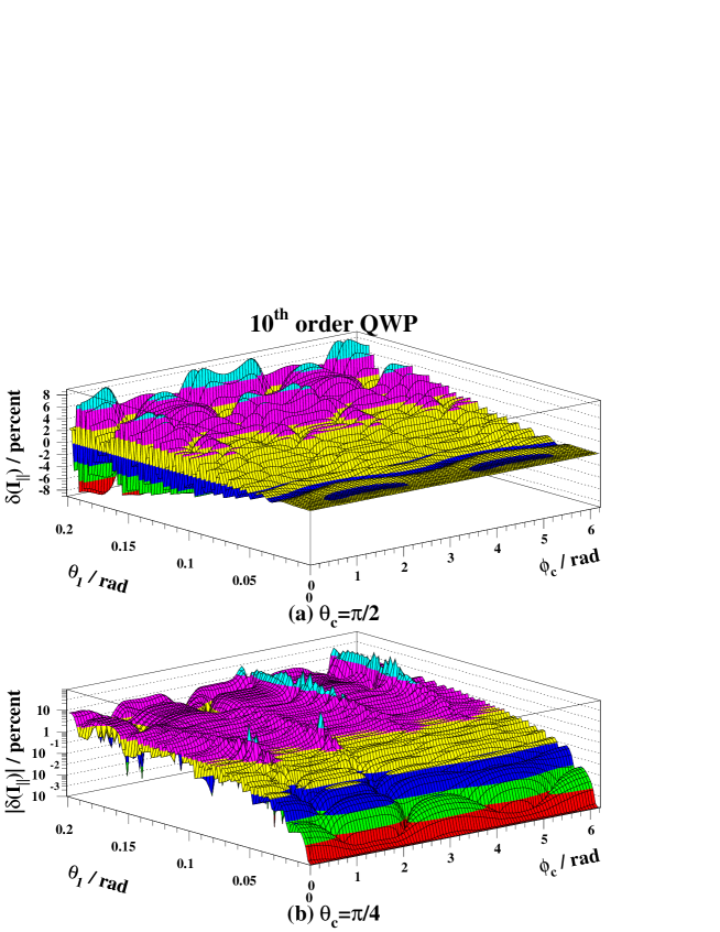
Fig. 6: Same a Fig.5 but the for the quantity of Fig.3.

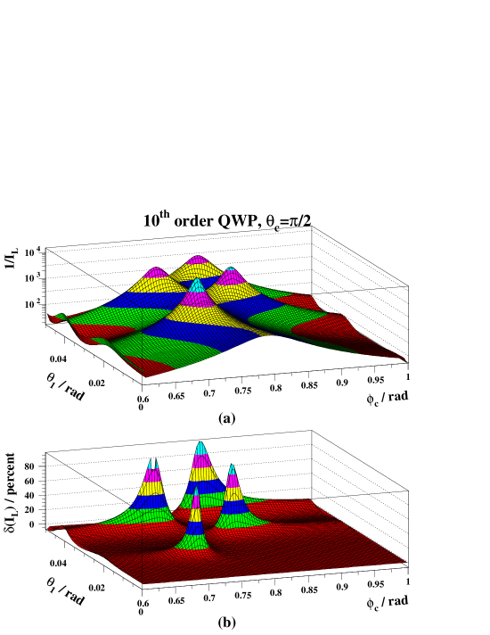
Fig. 7: (a) Inverse of the intensity measured after a tenth order QWP and a perfect circular left polarizer. Calculations are performed using the scalar Fourier approximation and are shown as function of the incident angle $\theta_{1}$ and the azimuth angle of the optical axis $\phi_{c}$. (b) Relative difference between the quantity shown in the top plot calculated using the scalar Fourier approximation and the plane wave approximation. For these figures, the optical axis is taken in the plane of interface ($\theta_{c}=\pi/2$).

Finally the ratio $\rho_{11}\rho_{21}/\rho_{11,21}$ is computed. It increases with $\theta_{1}$ and the plate thickness but, even for the tenth order QWP, it does not exceed 0.2 $\%$ for any values of $\phi_{c}$ and $\theta_{1}=0.2$ rad. Assuming $\rho_{11}\rho_{21}\approx\rho_{11,21}$, a Jones matrix can thus be defined with an accuracy of the order of a few per mill.

From this study one may conclude that:

• the scalar Fourier approximation is very accurate with respect to the paraxial approximation when the beam waist is not too small;

• the plane wave approximation mainly holds for thin Quartz plates, small incident angles, large beam waists and optical axes nearly in the interface plane. If these conditions are not fulfilled, an account for the Gaussian nature of the beam is necessary.

• It is crucial to account for the Gaussian nature of the beam when high performances of QWP are foreseen.

More generally, accuracies of the various approximations strongly depend on the medium birefringence and geometrical configurations.

6 conclusion

General expressions describing the transmission and reflection of a Gaussian beam by anisotropic parallel plates have been obtained. The vector Fourier optics formalism of Refs. ?, ? is used as general frame work. Multiple reflections inside the anisotropic medium are taken into account using a $2\times 2$ matrix algebra derived from the general $4\times 4$ matrix formalism of Ref.?. The only assumption supplied for these calculations is the paraxial approximation.

To simplify the calculations, a useful approximation introduced in Ref. ? is then considered. This approximation consist in taking into account the Gaussian nature of the beam only in the interference pattern of the transmitted (or reflected) beam. Birefringence effects induced by the beam angular divergence are then neglected. Accuracy of this approximation was checked for the particular case of uniaxial Quartz parallel plates. For not too small beam waists, no noticeable differences were observed compared to the general expression.

Precision of the plane wave approximation has also been checked using the example of Quartz plates. Here noticeable differences were observed. These discrepancies do not trivially depend on the geometrical parameters. Roughly, we concluded that they increase with the plate thickness and the angle of incidence. In the case of ellipsometry where a high purity circular polarization is foreseen, it was shown that an account for the Gaussian nature of the beam is necessary.

As a general remark, accuracies of the various approximations presented in this article decisively depend on the birefringence of the medium, laser wavelength, geometrical configuration and type of energy measurements. They must then be checked case by case.

Interference effects, observed in the variations of the transmitted beam intensity as function of the angle of incidence and optical axis azimuth, suggest that a very precise calibration of a birefringent plate can be performed without any other optical components.

7 Appendix I

In Ref. ?, the transmission of a Gaussian beam though a tilted Quartz plate has been determined. The configuration is restricted to a tilt axis perpendicular or parallel to the optical axis, itself located in the interface. In this appendix we show the equivalence between the results of Ref. ? and the formalism of section 4.

The elements of the transmission matrix are written

$$m_{oo} =\frac{t_{1{o}}t_{{o}1}\exp(-i(k_{y}\Delta_{o}+\delta_{o}))}{1-r_{o}^{2}\exp(-2i(k_{y}\Delta_{o}+\delta_{o}))}$$

$$m_{ee} =\frac{t_{1{e}}t_{{e}1}\exp(-i(k_{y}\Delta_{e}+\delta_{e}))}{1-r_{e}^{2}\exp(-2i(k_{y}\Delta_{e}+\delta_{e}))}$$

$$m_{oe} =m_{eo}=0$$

where $e$ and $o$ refer to the extraordinary and ordinary wave respectively. The non zero extended Mueller matrix elements are given by:

$$|\rho_{oo}|^{2} =\sqrt{\frac{w_{0}^{2}k^{2}}{2\pi}}\int|m_{oo}|^{2}\exp\biggl{(}\frac{-w_{0}^{2}k_{y}^{2}}{2}\biggr{)}dk_{y}$$ (36)

$$|\rho_{ee}|^{2} =\sqrt{\frac{w_{0}^{2}k^{2}}{2\pi}}\int|m_{ee}|^{2}\exp\biggl{(}\frac{-w_{0}^{2}k_{y}^{2}}{2}\biggr{)}dk_{y}$$ (37)

$$\rho_{oo;ee}\sin\phi_{oo;ee} =\frac{1}{2i}\int[m_{oo}m_{ee}^{*}-m_{oo}^{*}m_{ee}]\exp\biggl{(}\frac{-w_{0}^{2}k_{y}^{2}}{2}\biggr{)}dk_{y}$$

$$=\sqrt{\frac{w_{0}^{2}k^{2}}{2\pi}}\int[\Re(m_{ee})\Im(m_{oo})-\Re(m_{oo})\Im(m_{ee})]\exp\biggl{(}\frac{-w_{0}^{2}k_{y}^{2}}{2}\biggr{)}dk_{y}$$ (38)

$$\rho_{oo;ee}\cos\phi_{oo;ee} =\frac{1}{2}\int[m_{oo}m_{ee}^{*}+m_{oo}^{*}m_{ee}]\exp\biggl{(}\frac{-w_{0}^{2}k_{y}^{2}}{2}\biggr{)}dk_{y}$$

$$=\sqrt{\frac{w_{0}^{2}k^{2}}{2\pi}}\int[\Re(m_{ee})\Re(m_{oo})+\Im(m_{oo})\Im(m_{ee})]\exp\biggl{(}\frac{-w_{0}^{2}k_{y}^{2}}{2}\biggr{)}dk_{y}$$

with $m_{ij}=\Re(m_{ij})+i\Im(m_{ij})$ and where $r_{e}$, $r_{o}$, $t_{e1}$, $t_{o1}$, $t_{1e}$, $t_{1o}$ are the Fresnel coefficients for the particular geometric configuration studied here (expressions can be found in Ref. ?).

In Ref. ? a Jones matrix

$$\begin{pmatrix}\sqrt{2a_{1}}&0\\ 0&\sqrt{2a_{2}}\exp\biggl{(}-i{\rm arcsin}\frac{a_{3}}{\sqrt{a_{1}a_{2}}}\biggr{)}\\ \end{pmatrix}$$ (39)

is defined and expressions for $a_{1}$, $a_{2}$ and $a_{3}$ are provided (Eqs. (A16a), (A16b) and (A16c) in Appendix I of Ref. ?).

To demonstrate the equivalence between our approach and the one of Ref. ? we must show that Eqs. (36), (37) and (38) are integral forms of $2a_{1}$, $2a_{2}$ and $2a_{3}$ respectively. In order to prove it one just has to expand the integral kernels and then perform the integration over $k_{y}$. Since the scalar Fourier approximation was implicitly assumed in Ref. ?, one finds:

$$\frac{|\rho_{oo}|^{2}}{2}= \frac{t^{2}_{x}}{2}\biggl{(}1+r_{x}^{2}\biggl{[}1+2\cos(4\varphi_{x})\exp\biggl{(}\frac{-2\Delta^{2}}{w_{0}^{2}}\biggr{)}\biggr{]}+$$

$$2r_{x}^{3}\biggl{[}\cos(2\varphi_{x})\exp\biggl{(}\frac{-\Delta^{2}}{2w_{0}^{2}}\biggr{)}+\cos(6\varphi_{x})\exp\biggl{(}\frac{-9\Delta^{2}}{2w_{0}^{2}}\biggr{)}\biggr{]}$$

$$+r_{x}^{4}\biggl{[}1+2\cos(4\varphi_{x})\exp\biggl{(}\frac{-2\Delta^{2}}{w_{0}^{2}}\biggr{)}+2\cos(8\varphi_{x})\exp\biggl{(}\frac{-8\Delta^{2}}{w_{0}^{2}}\biggr{)}\biggr{]}+\cdots\biggl{)}$$ (40)

where notations of Ref. ? $r_{x}=r_{o}^{2}$, $t_{x}=t_{1o}t_{o1}$, $\varphi_{x}=\delta_{e}$, $\varphi_{x}=\delta_{o}$ and $\Delta\approx 2\Delta_{o}\approx 2\Delta_{e}$ have been adopted. Eq. (40) can be further written as a series, and this leads to Eq. (A16a) of Ref. ?.

The series expansion of $|\rho_{ee}|^{2}/2$ is obviously obtained by replacing $r_{x}$ and $t_{x}$ by $r_{y}=r_{e}^{2}$ and $t_{y}=t_{1e}t_{e1}$ respectively in Eq. (40). This leads to Eq. (A16b) of Ref. ?.

In the same way one finally obtains

$$\frac{\rho_{oo;ee}}{2}\sin\phi_{oo;ee}=\frac{t_{x}t_{y}}{2}\biggl{\{}-\sin(\varphi_{x}-\varphi_{y})+\exp\biggl{(}\frac{-\Delta^{2}}{2w_{0}^{2}}\biggr{)}\biggl{(}r_{x}\sin(3\varphi_{x}-\varphi_{y})-r_{y}\sin(3\varphi_{y}-\varphi_{x})\biggr{)}+$$

$$r_{x}r_{y}\biggl{[}-\sin(3[\varphi_{x}-\varphi_{y}])+\exp\biggl{(}\frac{-\Delta^{2}}{2w_{0}^{2}}\biggr{)}\biggl{(}r_{y}\sin(5\varphi_{y}-3\varphi_{x})-r_{x}\sin(5\varphi_{x}-3\varphi_{y})\biggr{)}+$$

$$\exp\biggl{(}\frac{-2\Delta^{2}}{w_{0}^{2}}\biggr{)}\biggl{(}\frac{r_{y}}{r_{x}}\sin(5\varphi_{y}-\varphi_{x})-\frac{r_{x}}{r_{y}}\sin(5\varphi_{x}-\varphi_{y})\biggr{)}+$$

$$\exp\biggl{(}\frac{-9\Delta^{2}}{2w_{0}^{2}}\biggr{)}\biggl{(}\frac{r_{y}^{2}}{r_{x}}\sin(7\varphi_{y}-\varphi_{x})-\frac{r_{x}^{2}}{r_{y}}\sin(7\varphi_{x}-\varphi_{y})\biggr{)}\biggr{]}+\cdots\biggr{\}}$$

which leads to Eq. (A16c) of Ref. ?.

Let us mention that, as stated in section 4, Eq. (39) represents the Jones matrix of a quarter wave plate only under the approximation $\rho_{oo,ee}\approx\rho_{oo}\rho_{ee}$.

8 Appendix II

In this appendix, ingredients for the calculation of the double integral of Eq. (25) are given.

Following Ref. ? we write

$$\mbox{${\rm\bf\hat{c}}$ }=\sin\theta_{c}\cos\phi_{c}\mbox{${\rm\bf\hat{x}_{I}}$ }+\sin\theta_{c}\sin\phi_{c}\mbox{${\rm\bf\hat{y}_{I}}$ }+\cos\theta_{c}\mbox{${\rm\bf\hat{z}_{I}}$ }$$

for the direction of the optical axis inside the Quartz plate. $\{\mbox{${\rm\bf\hat{x}_{I}}$ },\mbox{${\rm\bf\hat{y}_{I}}$ },\mbox{${\rm\bf\hat{z}_{I}}$ }\}$ is the basis attached to the Quartz plate (see Fig. 1). In this basis, the wave vectors of the plane wave (see Eq. (3)) and Gaussian beam center are given by:

$${\rm\bf k_{pw}} =k_{x}\mbox{${\rm\bf\hat{x}_{I}}$ }+(k_{y}\cos\theta_{1}+k_{z}\sin\theta_{1})\mbox{${\rm\bf\hat{y}_{I}}$ }+(k_{z}\cos\theta_{1}-k_{y}\sin\theta_{1})\mbox{${\rm\bf\hat{z}_{I}}$ }$$

$${\rm\bf k} =k\sin\theta_{1}\mbox{${\rm\bf\hat{y}_{I}}$ }+k\cos\theta_{1}\mbox{${\rm\bf\hat{z}_{I}}$ }$$

with $k_{z}\approx k(1-\mbox{$\rm\bf k^{2}_{\perp}$}/(2k^{2})))$. The plane wave incident and azimuth angles read

$$\cos\theta_{1pw}=\frac{k_{z}}{k}\cos\theta_{1}-\frac{k_{y}}{k}\sin\theta_{1},\,\,\tan\phi_{pw}=\frac{k_{z}\sin\theta_{1}+k_{y}\cos\theta_{1}}{k_{x}}.$$

The ordinary and extraordinary wave vectors corresponding to ${\rm\bf k_{pw}}$ and ${\rm\bf\hat{c}}$ are determined using the compact expression of Ref. ?. The electric polarization vectors inside the plate are determined using the general formula of Ref. ?.

Expressions for the interface matrices of Eqs. (17-22) are formally determined thanks to the Mapple software package .${}^{\hbox{\immediate{\bf{?}}}}$ These expressions are much too lengthy to be reproduced here.

The rotation matrix $\Omega$ (see Eq. (10)) is obtained from

$${\rm\bf\hat{s}_{pw}} = N_{s}[(k_{y}\cos\theta_{1}+k_{z}\sin\theta_{1})\mbox{${\rm\bf\hat{x}}$ }-k_{x}\cos\theta_{1}\mbox{${\rm\bf\hat{y}}$ }-k_{x}\sin\theta_{1}\mbox{${\rm\bf\hat{z}}$ }]$$

$${\rm\bf\hat{p}_{pw}} = N_{p}[(k_{x}k_{z}\cos\theta_{1}-k_{x}k_{y}\sin\theta_{1})\mbox{${\rm\bf\hat{x}}$ }+(k_{y}k_{z}\cos\theta_{1}+k_{z}^{2}\sin\theta_{1}+k_{x}^{2}\sin\theta_{1})\mbox{${\rm\bf\hat{y}}$ }$$

$$+(-\mbox{$\rm\bf k_{\perp}$}^{2}\cos\theta_{1}-k_{y}k_{z}\sin\theta_{1})\mbox{${\rm\bf\hat{z}}$ }]$$

$${\rm\bf\hat{k}_{pw}} = N_{k}[k_{x}\mbox{${\rm\bf\hat{x}}$ }+k_{y}\mbox{${\rm\bf\hat{y}}$ }+k_{z}\mbox{${\rm\bf\hat{z}}$ }]$$

where $N_{s}$, $N_{p}$ and $N_{k}$ are normalization factors.

References

• [1] R.M.A. Azzam and N.M. Bashara, Ellipsometry and polarized light (Amsterdam, North-Holland, 1977).
• [2] J. Poirson et al., “Jones matrix of a quarter-wave plate for Gaussian beams”, Appl. Opt. 34, 6806-6818 (1995).
• [3] E.C.G. Sudarshan, R. Simon and N. Mukunda, “Paraxial-wave optics and relativistic front description. I. The scalar theory” Phys. Rev. A 28, 2921-2932 (1983).
• [4] N. Mukunda, R. Simon and E.C.G. Sudarshan, “Paraxial-wave optics and relativistic front description. I. The vector theory”, Phys. Rev. A 28, 2933-2942 (1983).
• [5] P. Yeh, “Electromagnetic propagation in birefringent media”, J. Opt. Soc. Am. 69, 742-756 (1979); P. Yeh, “Optics of anisotropic layered media: a new $4\times 4$ matrix algebra”, Surf. Sci. 96, 41-53 (1980).
• [6] R. Simon, E.C.G. Sudarshan and N. Mukunda, “Cross polarization in laser beams”, Appl. Opt. 26, 1589-1593 (1987).
• [7] H. Bacry and M. Cadihac, “Metaplectic group and Fourier optics”, Phys. Rev. A 23, 2533-2536 (1981).
• [8] Y. Fainman and J. Shamir, “Polarization of nonplanar wave fronts”, Appl. Opt. 23, 3188-3195 (1984).
• [9] N. Mukunda, R. Simon and E.C.G. Sudarshan, “Paraxial Maxwell beams: transformation by general linear optical systems”, J. Opt. Soc. Am. A 2, 1291-1296 (1985).
• [10] S. Huard, Polarisation de la lumière (Masson, Paris, 1993).
• [11] M. Bass et al. Handbook of optics, Vol. II (Mc Graw-Hill, New-York, 1995).
• [12] X. Zhu, “Explicit Jones transformation matrix for a tilted birefringent plate with its optic axis parallel to the plate interface”, Appl. opt. 33, 3502-3506 (1994).
• [13] P. Yeh, “Extended Jones matrix method”, J. Opt. Soc. Am. 72, 507-513 (1982).
• [14] C. Gu and P. Yeh, “Extended Jones matrix method. II”, J. Opt. Soc. Am. A10, 966-973 (1993).
• [15] K. Zander, J. Moser and H. Melle, “Change of polarization of linearly polarized, coherent light transmitted through plane-parallel anisotropic plates”, Optik 70, 6-13 (1985).
• [16] Maple V software program (Waterloo Maple Inc., Ontario, Canada).