EUROPEAN ORGANIZATION FOR NUCLEAR RESEARCH

CERN-EP/2002-063

25 July 2002

Search for Nearly Mass-Degenerate Charginos and Neutralinos at LEP

The OPAL Collaboration

Abstract

A search was performed for charginos with masses close to the mass of the lightest neutralino in $\mathrm{e}^{+}\mathrm{e}^{-}$ collisions at centre-of-mass energies of 189–209 $\mathrm{GeV}$ recorded by the OPAL detector at LEP. Events were selected if they had an observed high-energy photon from initial state radiation, reducing the dominant background from two-photon scattering to a negligible level. No significant excess over Standard Model expectations has been observed in the analysed data set corresponding to an integrated luminosity of 570 pb^-1. Upper limits were derived on the chargino pair-production cross-section, and lower limits on the chargino mass were derived in the context of the Minimal Supersymmetric Extension of the Standard Model for the gravity and anomaly mediated Supersymmetry breaking scenarios.

(To be submitted to Eur. Phys. J.)

The OPAL Collaboration

G. Abbiendi², C. Ainsley⁵, P.F. Åkesson³, G. Alexander²², J. Allison¹⁶, P. Amaral⁹, G. Anagnostou¹, K.J. Anderson⁹, S. Arcelli², S. Asai²³, D. Axen²⁷, G. Azuelos^18,a, I. Bailey²⁶, E. Barberio⁸, R.J. Barlow¹⁶, R.J. Batley⁵, P. Bechtle²⁵, T. Behnke²⁵, K.W. Bell²⁰, P.J. Bell¹, G. Bella²², A. Bellerive⁶, G. Benelli⁴, S. Bethke³², O. Biebel³¹, I.J. Bloodworth¹, O. Boeriu¹⁰, P. Bock¹¹, D. Bonacorsi², M. Boutemeur³¹, S. Braibant⁸, L. Brigliadori², R.M. Brown²⁰, K. Buesser²⁵, H.J. Burckhart⁸, S. Campana⁴, R.K. Carnegie⁶, B. Caron²⁸, A.A. Carter¹³, J.R. Carter⁵, C.Y. Chang¹⁷, D.G. Charlton^1,b, A. Csilling^8,g, M. Cuffiani², S. Dado²¹, G.M. Dallavalle², S. Dallison¹⁶, A. De Roeck⁸, E.A. De Wolf⁸, K. Desch²⁵, B. Dienes³⁰, M. Donkers⁶, J. Dubbert³¹, E. Duchovni²⁴, G. Duckeck³¹, I.P. Duerdoth¹⁶, E. Elfgren¹⁸, E. Etzion²², F. Fabbri², L. Feld¹⁰, P. Ferrari⁸, F. Fiedler³¹, I. Fleck¹⁰, M. Ford⁵, A. Frey⁸, A. Fürtjes⁸, P. Gagnon¹², J.W. Gary⁴, G. Gaycken²⁵, C. Geich-Gimbel³, G. Giacomelli², P. Giacomelli², M. Giunta⁴, J. Goldberg²¹, E. Gross²⁴, J. Grunhaus²², M. Gruwé⁸, P.O. Günther³, A. Gupta⁹, C. Hajdu²⁹, M. Hamann²⁵, G.G. Hanson⁴, K. Harder²⁵, A. Harel²¹, M. Harin-Dirac⁴, M. Hauschild⁸, J. Hauschildt²⁵, C.M. Hawkes¹, R. Hawkings⁸, R.J. Hemingway⁶, C. Hensel²⁵, G. Herten¹⁰, R.D. Heuer²⁵, J.C. Hill⁵, K. Hoffman⁹, R.J. Homer¹, D. Horváth^29,c, R. Howard²⁷, P. Hüntemeyer²⁵, P. Igo-Kemenes¹¹, K. Ishii²³, H. Jeremie¹⁸, P. Jovanovic¹, T.R. Junk⁶, N. Kanaya²⁶, J. Kanzaki²³, G. Karapetian¹⁸, D. Karlen⁶, V. Kartvelishvili¹⁶, K. Kawagoe²³, T. Kawamoto²³, R.K. Keeler²⁶, R.G. Kellogg¹⁷, B.W. Kennedy²⁰, D.H. Kim¹⁹, K. Klein¹¹, A. Klier²⁴, S. Kluth³², T. Kobayashi²³, M. Kobel³, S. Komamiya²³, L. Kormos²⁶, R.V. Kowalewski²⁶, T. Krämer²⁵, T. Kress⁴, P. Krieger^6,l, J. von Krogh¹¹, D. Krop¹², K. Kruger⁸, M. Kupper²⁴, G.D. Lafferty¹⁶, H. Landsman²¹, D. Lanske¹⁴, J.G. Layter⁴, A. Leins³¹, D. Lellouch²⁴, J. Letts^o, L. Levinson²⁴, J. Lillich¹⁰, S.L. Lloyd¹³, F.K. Loebinger¹⁶, J. Lu²⁷, J. Ludwig¹⁰, A. Macpherson^28,i, W. Mader³, S. Marcellini², T.E. Marchant¹⁶, A.J. Martin¹³, J.P. Martin¹⁸, G. Masetti², T. Mashimo²³, P. Mättig^m, W.J. McDonald²⁸, J. McKenna²⁷, T.J. McMahon¹, R.A. McPherson²⁶, F. Meijers⁸, P. Mendez-Lorenzo³¹, W. Menges²⁵, F.S. Merritt⁹, H. Mes^6,a, A. Michelini², S. Mihara²³, G. Mikenberg²⁴, D.J. Miller¹⁵, S. Moed²¹, W. Mohr¹⁰, T. Mori²³, A. Mutter¹⁰, K. Nagai¹³, I. Nakamura²³, H.A. Neal³³, R. Nisius³², S.W. O’Neale¹, A. Oh⁸, A. Okpara¹¹, M.J. Oreglia⁹, S. Orito²³, C. Pahl³², G. Pásztor^4,g, J.R. Pater¹⁶, G.N. Patrick²⁰, J.E. Pilcher⁹, J. Pinfold²⁸, D.E. Plane⁸, B. Poli², J. Polok⁸, O. Pooth¹⁴, M. Przybycień^8,n, A. Quadt³, K. Rabbertz⁸, C. Rembser⁸, P. Renkel²⁴, H. Rick⁴, J.M. Roney²⁶, S. Rosati³, Y. Rozen²¹, K. Runge¹⁰, K. Sachs⁶, T. Saeki²³, O. Sahr³¹, E.K.G. Sarkisyan^8,j, A.D. Schaile³¹, O. Schaile³¹, P. Scharff-Hansen⁸, J. Schieck³², T. Schörner-Sadenius⁸, M. Schröder⁸, M. Schumacher³, C. Schwick⁸, W.G. Scott²⁰, R. Seuster^14,f, T.G. Shears^8,h, B.C. Shen⁴, C.H. Shepherd-Themistocleous⁵, P. Sherwood¹⁵, G. Siroli², A. Skuja¹⁷, A.M. Smith⁸, R. Sobie²⁶, S. Söldner-Rembold^10,d, S. Spagnolo²⁰, F. Spano⁹, A. Stahl³, K. Stephens¹⁶, D. Strom¹⁹, R. Ströhmer³¹, S. Tarem²¹, M. Tasevsky⁸, R.J. Taylor¹⁵, R. Teuscher⁹, M.A. Thomson⁵, E. Torrence¹⁹, D. Toya²³, P. Tran⁴, T. Trefzger³¹, A. Tricoli², I. Trigger⁸, Z. Trócsányi^30,e, E. Tsur²², M.F. Turner-Watson¹, I. Ueda²³, B. Ujvári^30,e, B. Vachon²⁶, C.F. Vollmer³¹, P. Vannerem¹⁰, M. Verzocchi¹⁷, H. Voss⁸, J. Vossebeld^8,h, D. Waller⁶, C.P. Ward⁵, D.R. Ward⁵, P.M. Watkins¹, A.T. Watson¹, N.K. Watson¹, P.S. Wells⁸, T. Wengler⁸, N. Wermes³, D. Wetterling¹¹ G.W. Wilson^16,k, J.A. Wilson¹, G. Wolf²⁴, T.R. Wyatt¹⁶, S. Yamashita²³, D. Zer-Zion⁴, L. Zivkovic²⁴

¹School of Physics and Astronomy, University of Birmingham, Birmingham B15 2TT, UK
²Dipartimento di Fisica dell’ Università di Bologna and INFN, I-40126 Bologna, Italy
³Physikalisches Institut, Universität Bonn, D-53115 Bonn, Germany
⁴Department of Physics, University of California, Riverside CA 92521, USA
⁵Cavendish Laboratory, Cambridge CB3 0HE, UK
⁶Ottawa-Carleton Institute for Physics, Department of Physics, Carleton University, Ottawa, Ontario K1S 5B6, Canada
⁸CERN, European Organisation for Nuclear Research, CH-1211 Geneva 23, Switzerland
⁹Enrico Fermi Institute and Department of Physics, University of Chicago, Chicago IL 60637, USA
¹⁰Fakultät für Physik, Albert-Ludwigs-Universität Freiburg, D-79104 Freiburg, Germany
¹¹Physikalisches Institut, Universität Heidelberg, D-69120 Heidelberg, Germany
¹²Indiana University, Department of Physics, Bloomington IN 47405, USA
¹³Queen Mary and Westfield College, University of London, London E1 4NS, UK
¹⁴Technische Hochschule Aachen, III Physikalisches Institut, Sommerfeldstrasse 26-28, D-52056 Aachen, Germany
¹⁵University College London, London WC1E 6BT, UK
¹⁶Department of Physics, Schuster Laboratory, The University, Manchester M13 9PL, UK
¹⁷Department of Physics, University of Maryland, College Park, MD 20742, USA
¹⁸Laboratoire de Physique Nucléaire, Université de Montréal, Montréal, Québec H3C 3J7, Canada
¹⁹University of Oregon, Department of Physics, Eugene OR 97403, USA
²⁰CLRC Rutherford Appleton Laboratory, Chilton, Didcot, Oxfordshire OX11 0QX, UK
²¹Department of Physics, Technion-Israel Institute of Technology, Haifa 32000, Israel
²²Department of Physics and Astronomy, Tel Aviv University, Tel Aviv 69978, Israel
²³International Centre for Elementary Particle Physics and Department of Physics, University of Tokyo, Tokyo 113-0033, and Kobe University, Kobe 657-8501, Japan
²⁴Particle Physics Department, Weizmann Institute of Science, Rehovot 76100, Israel
²⁵Universität Hamburg/DESY, Institut für Experimentalphysik, Notkestrasse 85, D-22607 Hamburg, Germany
²⁶University of Victoria, Department of Physics, P O Box 3055, Victoria BC V8W 3P6, Canada
²⁷University of British Columbia, Department of Physics, Vancouver BC V6T 1Z1, Canada
²⁸University of Alberta, Department of Physics, Edmonton AB T6G 2J1, Canada
²⁹Research Institute for Particle and Nuclear Physics, H-1525 Budapest, P O Box 49, Hungary
³⁰Institute of Nuclear Research, H-4001 Debrecen, P O Box 51, Hungary
³¹Ludwig-Maximilians-Universität München, Sektion Physik, Am Coulombwall 1, D-85748 Garching, Germany
³²Max-Planck-Institute für Physik, Föhringer Ring 6, D-80805 München, Germany
³³Yale University, Department of Physics, New Haven, CT 06520, USA

^a and at TRIUMF, Vancouver, Canada V6T 2A3
^b and Royal Society University Research Fellow
^c and Institute of Nuclear Research, Debrecen, Hungary
^d and Heisenberg Fellow
^e and Department of Experimental Physics, Lajos Kossuth University, Debrecen, Hungary
^f and MPI München
^g and Research Institute for Particle and Nuclear Physics, Budapest, Hungary
^h now at University of Liverpool, Dept of Physics, Liverpool L69 3BX, UK
ⁱ and CERN, EP Div, 1211 Geneva 23
^j and Universitaire Instelling Antwerpen, Physics Department, B-2610 Antwerpen, Belgium
^k now at University of Kansas, Dept of Physics and Astronomy, Lawrence, KS 66045, USA
^l now at University of Toronto, Dept of Physics, Toronto, Canada
^m current address Bergische Universität, Wuppertal, Germany
ⁿ and University of Mining and Metallurgy, Cracow, Poland
^o now at University of California, San Diego, U.S.A.

1 Introduction

Supersymmetric (SUSY) extensions [1, *Volkov:1973ix, *Wess:1974tw] of the Standard Model (SM) provide a promising approach to overcoming shortcomings of the SM. By introducing supersymmetric partners for each SM particle, differing in spin by 1/2 unit from the SM particles, the hierarchy problem can be solved and large radiative corrections to the Higgs mass cancel out. The simplest potentially realistic supersymmetric field theory is the Minimal Supersymmetric Extension of the Standard Model (MSSM), which introduces only a minimum set of additional particles. Among these new particles are the gauginos and higgsinos which are the fermionic partners of the gauge and Higgs bosons, respectively. The charginos ($\tilde{\chi}^{\pm}_{i=1,2}$) are the mass eigenstates formed by the mixing of the fields of the charged gauginos and higgsinos. The neutralinos ($\tilde{\chi}^{0}_{j=1,\dots,4}$) are correspondingly formed by the mixing of the neutral gauginos and higgsinos.

In this paper the hypothesis of $R$-parity conservation is made. $R$-parity conserving SUSY scenarios allow only the pair-production of SUSY particles. In addition, there must exist a lightest, neutral, weakly interacting SUSY particle (LSP) which terminates the decay chain of any SUSY particle. In the following it is assumed that the lightest neutralino is the LSP. The lack of experimental evidence for supersymmetric particles leads to the assumption that SUSY particles are much heavier than their SM partners. Therefore, SUSY cannot be an exact symmetry of nature. If it exists it must be a broken symmetry. Further assumptions and constraints are imposed in order to reduce the large parameter space arising from the unknown mechanism of SUSY breaking. The results of this paper are interpreted within the gravity mediated SUSY breaking scenario (an expansion of the mSUGRA model [2, 3, *Arnowitt:1997um]) and the anomaly mediated SUSY breaking scenario (AMSB [4, 5]). While the former scenario offers an elegant way of explaining the breaking mechanism without additional fields or interactions, gravity mediated models in general suffer from large flavour changing neutral currents which must be removed by fine-tuning. Within the gravity mediated framework, we will consider both the so-called gaugino-scenario and higgsino-scenario which have different chargino production mechanisms and cross-sections. The AMSB scenario exploits the fact that rescaling anomalies in the supergravity Lagrangian always give rise to soft mass parameters and thus anomalies always contribute to the SUSY breaking mechanism.

If charginos exist and are sufficiently light, they can be pair-produced at LEP and may decay mainly via a virtual $\mathrm{W}$ boson into neutralinos and fermions. The kinematic properties of the final state particles, and therefore the event topologies, depend on the mass difference between chargino and neutralino, $\Delta M$. Chargino search strategies can be roughly categorised by the value of $\Delta M$. For large mass differences ($\Delta M\gtrsim 5\,\mathrm{GeV}$) the final state fermions are quarks or energetic leptons and the signal events can be identified by missing energy (carried away by the neutralinos) plus jets or isolated leptons. For very small mass differences ($\Delta M\lesssim M_{\pi}$) the chargino lifetime increases and the chargino decay vertex should be well separated from the interaction point. Heavy stable charged particles and/or secondary vertices are the signatures for this scenario. Searches for all these topologies were carried out by all LEP experiments [9, *Ackerstaff:1998si, 6, *Barate:1999gm, 7, *Abreu:2001mc, 8, *Acciarri:1999bw], but no evidence for a signal was found.

In this note, scenarios with a mass difference in the intermediate range ($0.17\,\mathrm{GeV}\lesssim\Delta M\lesssim 5\,\mathrm{GeV}$) are investigated. The searches for heavy stable charged particles have high efficiency and hence still some sensitivity to the $\Delta M$ region between $M_{\pi}$ and $0.17\,\mathrm{GeV}$. In the intermediate $\Delta M$ regime the signal final state is characterised by very little hadronic or leptonic activity accompanied by a large amount of missing energy. Events from two-photon processes give rise to a very large background which is difficult to suppress. However, due to the large predicted cross-sections for chargino pair-production, the search can be restricted to events which also have an energetic photon from initial state radiation (ISR). These are distinguishable from two-photon background [10, *Chen:1999yf]. This method was proposed in [11] for the search for heavy charged leptons which are nearly mass degenerate with their neutrino. Recent search results from other LEP experiments, using this method, are reported in [12, 13, 14].

Section 2 of this note describes the OPAL detector while Section 3 details the simulation of both signal and background events. Section 4 deals with event selection and Section 5 with systematic uncertainties. No evidence for chargino pair-production was found and the search results are interpreted in Section 6 in terms of upper limits on the production cross-section and in terms of lower mass-limits within the MSSM framework.

2 The OPAL Detector

The OPAL detector is described in detail in [15, *Anderson:1998xw, *Anderson:1994ve, 16]. It was a multipurpose apparatus with almost complete solid angle coverage. The central detector consisted of two layers of silicon strip detectors and a system of gas-filled tracking chambers in a 0.435 T solenoidal magnetic field which was parallel to the beam axis. The barrel time-of-flight scintillator bars were located outside the solenoid, and the end-caps were equipped with scintillating tiles [16]. The scintillator systems were surrounded by a lead-glass electromagnetic calorimeter (ECAL), which gave hermetic coverage in the region $|\cos\theta|<0.984$. The magnet return yoke was instrumented for hadron calorimetry. The forward region was covered by electromagnetic calorimeters, namely the silicon-tungsten calorimeter (SW, $25\,\mathrm{mrad}<\theta<59\,\mathrm{mrad}$), the forward detector (FD, $47\,\mathrm{mrad}<\theta\lesssim 160\,\mathrm{mrad}$) and the gamma catcher (GC, $143\,\mathrm{mrad}<\theta<193\,\mathrm{mrad}$). Taking into account material to shield the detector from accelerator related backgrounds, the detector was sensitive down to $\theta_{\mathrm{min}}=33\,\mathrm{mrad}$.

3 Data Sample and Monte Carlo Simulation

3.1 The Data Sample

The data analysed in this note were taken in 1998, 1999 and 2000 at centre-of-mass energies $\sqrt{s}$ between 188 and 209 $\mathrm{GeV}$. The search is based on a total of 569.9 $\mathrm{pb}^{-1}$ of data for which all relevant detector components were fully operational. The luminosity weighted mean centre-of-mass energy and the integrated luminosity of each energy bin is listed in Table 1.

year	$\sqrt{s}$ bin range	$\langle\sqrt{s}\rangle$	$\int\mathcal{L}\mathrm{d}t$
	$[\mathrm{GeV}]$	$[\mathrm{GeV}]$	$[\mathrm{pb}^{-1}]$
1998	188.0 – 190.5	188.6	167.6
1999	190.5 – 194.0	191.6	27.7
1999	194.0 – 199.0	195.5	71.2
1999	199.0 – 201.0	199.5	72.1
1999	201.0 – 202.5	201.6	33.9
2000	203.5 – 204.5	204.0	7.7
2000	204.5 – 205.5	205.2	64.9
2000	205.5 – 206.5	206.3	58.6
2000	206.5 – 207.5	206.7	58.9
2000	$>207.5$	208.1	7.3
			569.9

Table 1: The luminosity weighted mean centre-of-mass energy and integrated luminosity of each energy bin.

3.2 Signal Simulation

The SUSYGEN [17] generator was used to simulate the signal events. In this program initial state corrections are incorporated using a factorised “radiator formula” (REMT by Kleiss [18]) where exponentiation of higher orders and the transverse momentum distribution of the photon have been implemented. The generated chargino masses $M_{\tilde{\chi}^{\pm}_{1}}$ ranged from 45 $\mathrm{GeV}$ to 97.5 $\mathrm{GeV}$. The step size was 5 $\mathrm{GeV}$ for $M_{\tilde{\chi}^{\pm}_{1}}\leq 80\,\mathrm{GeV}$. Above this mass the step size was reduced to $2.5\,\mathrm{GeV}$. The simulated mass differences were $\Delta M$=0.17, 0.2, 0.3, 0.4, 0.5, 1.0, 1.5, 2.0, 3.0, 4.0 and 5.0 $\mathrm{GeV}$. The points were chosen to give a ($M_{\tilde{\chi}^{\pm}_{1}}$, $\Delta M$) grid covering all points at which a reasonable signal efficiency was expected, also taking into account existing chargino mass limits from LEP 1. A total of 500 signal events were generated for each grid point at $\sqrt{s}=$189, 192, 196, 200, 202, 204, 205, 206, 207 and 208 $\mathrm{GeV}$, and for both the higgsino-like and gaugino-like scenarios, in view of their different ISR spectrum shapes. The signal events were required to be accompanied by one ISR photon within the ECAL acceptance $|\cos\theta|<0.984$. The transverse momentum of the ISR photon was required to be larger than $0.025\,\sqrt{s}$.

The chargino decay width implemented in SUSYGEN was modified. New hadronic chargino decay channels ($\tilde{\chi}^{-}_{1}\to\pi^{-}\tilde{\chi}^{0}_{1}$, $\tilde{\chi}^{-}_{1}\to\pi^{-}\pi^{0}\tilde{\chi}^{0}_{1}$ and $\tilde{\chi}^{-}_{1}\to\pi^{-}\pi^{-}\pi^{+}\tilde{\chi}^{0}_{1}$) were added reflecting analytical calculations described in [10, *Chen:1999yf, 19]. The hadronic $\tilde{\chi}^{\pm}_{1}$ decays are modelled using these channels as long as the sum of their partial widths is larger than the width of the tree level $\tilde{\chi}^{\pm}_{1}\to\mbox{$\mathrm{q\overline{q}^{\prime}}$}\tilde{\chi}^{0}_{1}$ decay. The $\tilde{\chi}^{\pm}_{1}\to\mbox{$\mathrm{q\overline{q}^{\prime}}$}\tilde{\chi}^{0}_{1}$ decay mode dominates for $\Delta M\gtrsim 1.5\,\mathrm{GeV}$.

3.3 Background Simulation

The following background processes were considered: lepton pairs ($\mathrm{e}^{+}\mathrm{e}^{-}\to{(\mathrm{Z}^{0}/\gamma)}^{\star}\to\ell\bar{\ell}$), multi-hadronic ($\mathrm{e}^{+}\mathrm{e}^{-}\to{(\mathrm{Z}^{0}/\gamma)}^{\star}\to\mathrm{q}\bar{\mathrm{q}}$), four-fermion ($\mathrm{e}^{+}\mathrm{e}^{-}\to\mathrm{f}\bar{\mathrm{f}}\mathrm{f}\bar{\mathrm{f}}$) and two-photon ($\mathrm{e}^{+}\mathrm{e}^{-}\to\mathrm{e}^{+}\mathrm{e}^{-}\gamma\gamma\to\mathrm{e}^{+}\mathrm{e}^{-}X$) processes.

KK2F [20] was used to simulate $\tau^{+}\tau^{-}(\gamma)$, $\mu^{+}\mu^{-}(\gamma)$ and multi-hadronic final states. NUNUGPV [21] was used to generate $\nu\bar{\nu}(\gamma)$ events. TEEGG [22] and BHWIDE [23] were used to simulate $\mathrm{e}^{+}\mathrm{e}^{-}(\gamma)$ events. RADCOR [24] was used to simulate photon pair final states. KORALW [25, *Skrzypek:1996ur] and grc4f [26] were used to generate four-fermion events. The latter was used for all four-fermion final states involving $\mathrm{e}^{+}\mathrm{e}^{-}$ pairs. Both KORALW and grc4f simulate ISR, but only the KORALW samples include ISR photons with transverse momentum.

PHOJET [27, *Engel:1995sb, *Engel:1996yd], HERWIG [28] and VERMASEREN [29] were used to simulate two-photon collisions resulting in electron pair or hadronic final states. None of these Monte Carlo generators include QED radiative corrections. The generator of Berends, Darverveldt and Kleiss (BDK) [30, *Berends:1986if, *Berends:1986ig, *Berends:1986ih] is able to handle these corrections. The program was written to simulate $\mathrm{e}^{+}\mathrm{e}^{-}\to\mathrm{e}^{+}\mathrm{e}^{-}\gamma^{\star}\gamma^{\star}(\gamma)\to\mathrm{e}^{+}\mathrm{e}^{-}\mu^{+}\mu^{-}(\gamma)$ events. For this analysis BDK was modified to allow the generation of $\tau$ final states. While for the $\tau$ samples no cuts were applied at generator level, in the case of the $\mu$ samples an event was accepted if it satisfied one of the following three requirements: it contained at least one particle with $|\cos\theta|<0.975$ and a transverse momentum (with respect to the beam axis) larger than 4.0 $\mathrm{GeV}$ or it contained two particles with $|\cos\theta|<0.975$ and the total missing transverse momentum (with respect to the beam axis) of the event was larger than 1.0 $\mathrm{GeV}$ or it contained more than two particles with $|\cos\theta|<0.975$. Since BDK includes only the QED coupling of photons, it cannot be used to describe all features of two-photon processes, e.g. the hadron-like structure of photons. Therefore no attempt was made to fully model the background from radiative hadronic two-photon events. However, BDK was used to verify that the veto on these events operates efficiently. The veto cuts (see Section 4.1.2) depend predominantly on the characteristics of the ISR photon and the beam electrons and not on the properties of the two-photon system.

Unless specified, JETSET 7.4 [31, *Sjostrand:1994yw] was used for the fragmentation of final states involving quarks. The number of events generated was typically well above the number expected in data. All Monte Carlo events generated were passed through a complete simulation of the OPAL detector [32], and processed in the same way as the data.

4 The Analysis

Signal events from the process $\mbox{$\mathrm{e}^{+}\mathrm{e}^{-}$}\to\tilde{\chi}^{+}_{1}\tilde{\chi}^{-}_{1}\gamma\to\tilde{\chi}^{0}_{1}\tilde{\chi}^{0}_{1}\gamma+X$ are characterised by an energetic photon accompanied by large missing energy and momentum and little hadronic or leptonic activity. The photon increases the total visible energy of the event and guarantees a high trigger efficiency ($\sim 100\%$). Since only a small fraction of signal events are accompanied by a hard ISR photon the signal efficiency is expected to be rather low. However, given the high integrated luminosities of the LEP 2 data samples a signal would still be observable.

Radiative two-photon events $\mbox{$\mathrm{e}^{+}\mathrm{e}^{-}$}\to\mbox{$\mathrm{e}^{+}\mathrm{e}^{-}$}\gamma+X$ can lead to a similar topology to the signal. However, in this case a final state electron can also be observed if it has a polar angle larger than $\theta_{\mathrm{min}}$. This angle can be related to the minimum transverse energy $E_{\mathrm{T}}^{\gamma\mathrm{min}}$ of the detected photon [33]:

$$E_{\mathrm{T}}^{\gamma}\gtrsim{E_{\mathrm{T}}^{\gamma}}^{\mathrm{min}}=\sqrt{s}\frac{\sin\theta_{\mathrm{min}}}{1+\sin\theta_{\mathrm{min}}}.$$ (1)

Therefore, requiring a photon with $E_{\mathrm{T}}^{\gamma}>{E_{\mathrm{T}}^{\gamma}}^{\mathrm{min}}$ in the final state allows an efficient reduction of two-photon processes by vetoing events with a scattered beam electron. The expression in Eq. (1) is an approximation, which allows for resolution effects.

Unless specified, the same quality requirements for tracks and ECAL clusters were used as in [34]. Double-counting of energy between tracks and calorimeter clusters was corrected as in [35]. This procedure results in a set of reconstructed particles. Photons were identified by an algorithm similar to that described in detail in [36, *Abbiendi:1999aa]. Photon candidates were identified as one of three types:

• A photon candidate was defined as an ECAL cluster including at least two lead-glass blocks, and with no reconstructed track compatible with being associated with the cluster. Furthermore, the energy of additional tracks and clusters in a $15^{\circ}$ half-angle cone defined by the photon direction had to be less than 2 $\mathrm{GeV}$. The photon candidate was accepted if $|\cos\theta^{\gamma}|<0.976$. If several photon candidates were found they were ordered according to their energy beginning with the highest energy.

• Two-track photon conversions were selected using an artificial neural network.

• Conversions where only a single track was reconstructed were defined as an ECAL cluster associated with a reconstructed track which was consistent with pointing to the primary vertex.

For this analysis only non-converted ISR photon candidates were considered.

4.1 Event Selection

4.1.1 Pre-Selection

Events were selected if a photon candidate was found in the ECAL. The photon transverse energy had to be larger than 5 $\mathrm{GeV}$. In order to reduce the background the reduced visible energy, $E_{\mathrm{vis}}$, defined as the difference between total visible energy and the photon candidate energy, $E^{\gamma}$, was required to be less than $0.35\,\sqrt{s}$. High-multiplicity events were rejected by requiring that the number of tracks passing the track quality cuts [34], excluding tracks which had been assigned to a photon conversion, had to be at least two and at most ten. In addition beam-gas and beam-wall interactions and cosmic background were rejected by a veto described in [37] using ECAL cluster shapes, information from the time-of-flight system, the tile end-cap scintillators, the muon chambers and the hadronic calorimeter. After this rather loose pre-selection all events had to pass the veto on two-photon events (V), a more refined cleaning selection (C), and a final selection (F). If events contained more than one photon candidate the chain of cuts was repeated for each photon separately starting with the one with the highest energy until one candidate was found passing all cuts or all candidates failed one cut.

4.1.2 The Two-Photon Veto

Two-photon events were vetoed by additional energy deposited in the detector from a final state electron (“two-photon veto”).

• The photon candidate had to pass the $E_{\mathrm{T}}^{\gamma}$ requirement Eq. (1). With a minimal accessible electron polar angle of $\theta_{\mathrm{min}}=33$ mrad the transverse photon energy was required to satisfy ${E_{\mathrm{T}}^{\gamma}}\geqslant 0.0319\sqrt{s}$.

• The sum of energies, $E_{\mathrm{fwd}}$, detected in the forward detectors SW, FD, GC on either side had to be smaller than 5 $\mathrm{GeV}$.

From the two-photon samples produced with the BDK generator a two-photon veto efficiency of $\varepsilon^{\gamma\gamma}>99.9\%$ was derived.

4.1.3 Cleaning Cuts

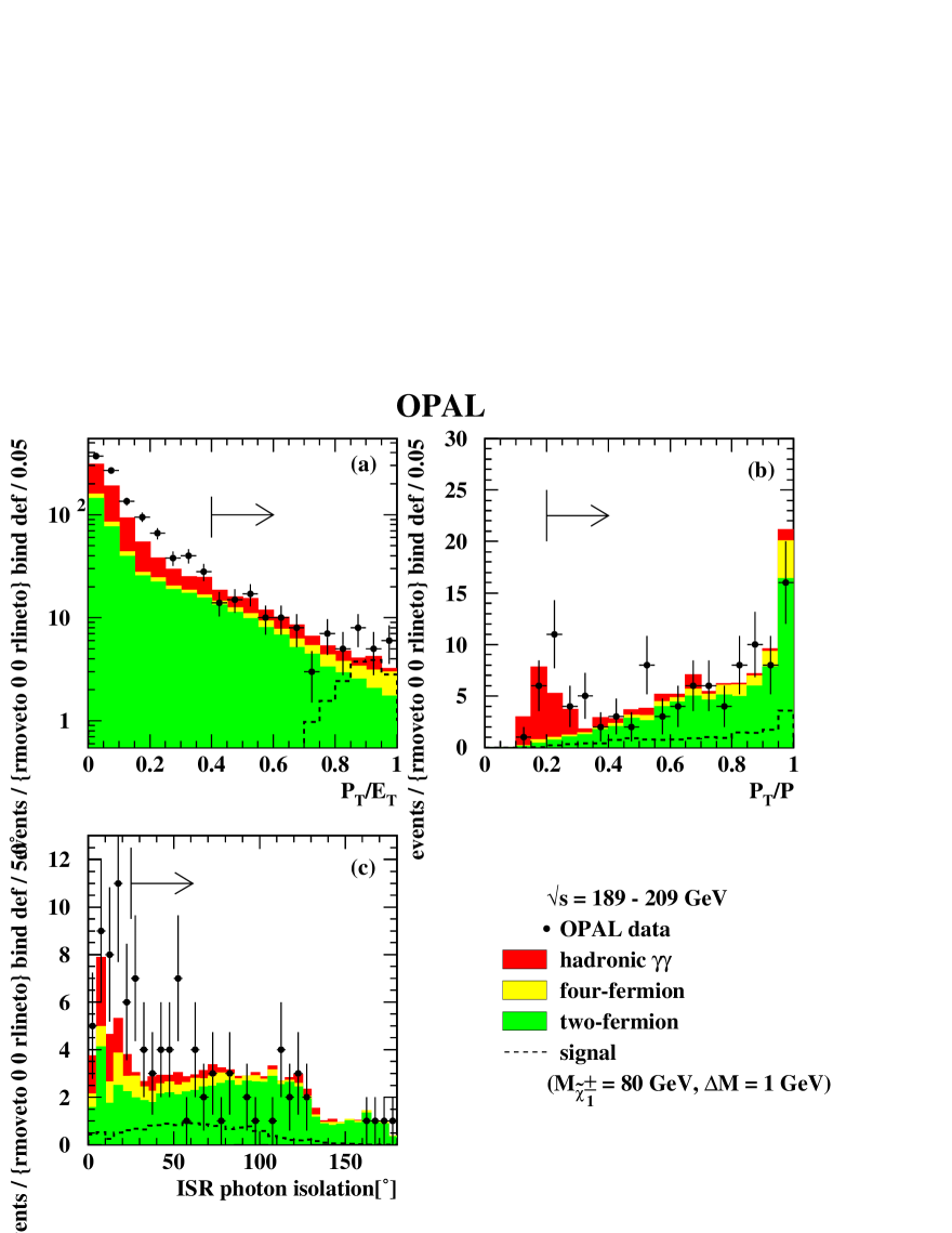
Figure 1: Variables used as cleaning cuts. The OPAL data are indicated by points with error bars (statistical error) and the background distributions by the histograms. Signal distributions are plotted as dashed lines and correspond to a chargino with $M_{\tilde{\chi}^{\pm}_{1}}=80\,\mathrm{GeV}$ and $\Delta M=1\,\mathrm{GeV}$. The accumulated events for $\sqrt{s}=$189 – 209 $\mathrm{GeV}$ are shown. Each plot shows the distribution after the cuts on the preceeding variables. The arrows indicate the accepted regions.

After the pre-selection and the two-photon veto, the remaining events in the background sample are mainly hadronic two-photon events with a faked or misinterpreted ISR photon, or from two-fermion events. Figure 1 shows the distributions of the variables used for the cleaning cuts against this background. The cut variables are based mainly on the properties of the reconstructed particles: The total transverse momentum $P_{\mathrm{T}}$ is the component of the total momentum $P$ (including the ISR candidate) transverse to the beam axis. The transverse visible energy $E_{\mathrm{T}}$ was calculated by summing up the absolute transverse momenta (with respect to the beam axis) of all reconstructed particles.

• Most of the events from hadronic two-photon processes and two-fermion events were removed by demanding that the ratio of the total transverse momentum to the transverse energy $P_{\mathrm{T}}/E_{\mathrm{T}}$ is larger than 0.4.

• A further reduction of the hadronic two-photon background was achieved by requiring that the ratio of the total transverse momentum to the total momentum $P_{\mathrm{T}}/P$ is larger than 0.2.

• The definition of a photon candidate was further restricted with the following cuts. The relative photon energy measurement error had to be less than $30\%$. In addition the angle between the photon candidate and any track or ECAL cluster was required to be larger then $25^{\circ}$.

As shown in Figure 1 the agreement between data and Monte Carlo is poor, but this is expected due to the unmodelled ISR spectrum in most of the Monte Carlo samples and the uncertainty on the two-photon cross-sections. However, the largest disagreement lies outside the accepted regions.

4.1.4 The Final Selection

To optimise the signal to background ratio, the final two cuts are a function of the point in the ($M_{\tilde{\chi}^{\pm}_{1}}$, $\Delta M$) space which is being tested.

• The ISR photon candidate recoil mass is defined as $M_{\mathrm{rec}}=\sqrt{s}(1-2E^{\gamma}/\sqrt{s})^{\frac{1}{2}}$. The recoil mass should be at least twice the tested chargino mass $M_{\tilde{\chi}^{\pm}_{1}}$. Taking resolution effects into account the cut on the recoil mass was set to $2\times M_{\tilde{\chi}^{\pm}_{1}}-2.5\,\mathrm{GeV}$.

• The visible energy $E_{\mathrm{vis}}$ depends to first order on the tested mass difference $\Delta M$. In order to retain the maximum signal efficiency, $E_{\mathrm{vis}}$ was required to be smaller than $4\times\Delta M$.

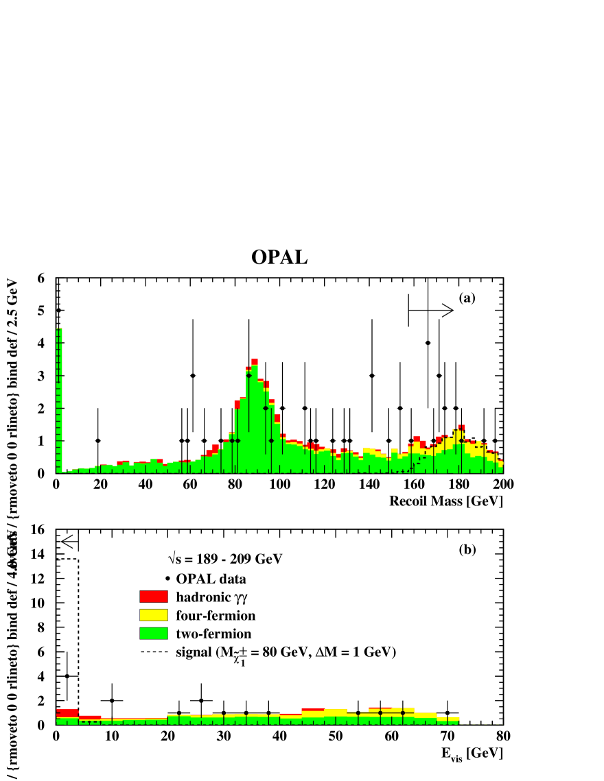
Figure 2: Variables used in the final event selection. The OPAL data are indicated by points with error bars (statistical error) and the background distributions by the histograms. Signal distributions are plotted as dashed lines and correspond to a chargino with $M_{\tilde{\chi}^{\pm}_{1}}=80\,\mathrm{GeV}$ and $\Delta M=1\,\mathrm{GeV}$. The accumulated events for $\sqrt{s}=$189 – 209 $\mathrm{GeV}$ are shown. Each plot shows the distribution after the cuts on the preceeding variables. The arrows indicate the accepted regions.

The recoil mass distribution after cut C3 and the visible energy distribution after cut F1 are shown in Figure 2.

4.2 Selection Results

The numbers of observed events and expected background events after each cut for the full available data set ($\sqrt{s}=$189 – 209 $\mathrm{GeV}$) are summarised in Table 2. The disagreement between data and Monte Carlo during the pre-selection vanishes after the two-photon veto. After the final cut F2 no excess over the SM background is observed.

	two-fermion	four-fermion	two-photon	total bkg.	data
P	$584.7\pm 8.4$	$69.2\pm 1.1$	$923.0\pm 13.5$	$1580\pm 16$	2432
V1	$561.0\pm 8.2$	$63.1\pm 1.1$	$607.9\pm 9.9$	$1235\pm 13$	1881
V2	$427.8\pm 7.3$	$47.4\pm 0.9$	$393.2\pm 8.0$	$870.7\pm 10.9$	1150
C1	$71.0\pm 0.9$	$12.9\pm 0.4$	$24.4\pm 1.3$	$108.3\pm 1.6$	108
C2	$70.6\pm 0.9$	$12.4\pm 0.4$	$14.4\pm 1.0$	$97.4\pm 1.4$	101
C3	$58.4\pm 0.8$	$8.1\pm 0.3$	$5.4\pm 0.6$	$72.0\pm 1.0$	52
F1	$9.7\pm 0.3$	$5.5\pm 0.3$	$1.5\pm 0.3$	$16.7\pm 0.5$	16
F2	$0.5\pm 0.1$	$0.09\pm 0.02$	$0.7\pm 0.2$	$1.3\pm 0.2$	4

Table 2: Number of expected background events and number of candidates after each cut. The first three rows list the contributions to the expected background from fermion-pair, four-fermion and two-photon events. The hadronic two-photon events passing the two-photon veto are those produced with generators without QED radiative corrections. The errors are statistical. All numbers correspond to the full analysed data set (569.9 pb^-1). For the final cuts F1 and F2 a chargino mass of $M_{\tilde{\chi}^{\pm}_{1}}=80\,\mathrm{GeV}$ and a mass difference of $\Delta M=1\,\mathrm{GeV}$ were assumed.

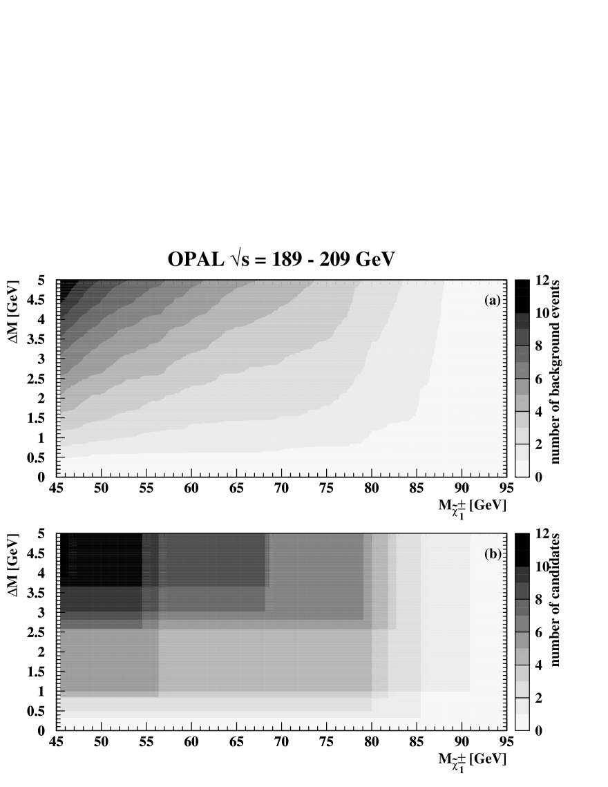
Figure 3: Number of expected background events (a) and number of candidates (b) passing the final selection cuts. The accumulated events for $\sqrt{s}=$189 – 209 $\mathrm{GeV}$ are shown.

The numbers of candidates and expected events after the final cut F2 for a selection of ($M_{\tilde{\chi}^{\pm}_{1}}$, $\Delta M$) grid points are listed in Table 3. The distribution of candidates and expected events in the ($M_{\tilde{\chi}^{\pm}_{1}}$,$\Delta M$) plane is illustrated in Figure 3.

$M_{\tilde{\chi}^{\pm}_{1}}\,[\mathrm{GeV}]$	$\Delta M\,[\mathrm{GeV}]$	total bkg.	data
50	4	$7.3\pm 0.5$	10
60	3	$4.1\pm 0.4$	6
70	2	$2.4\pm 0.3$	4
80	1	$1.3\pm 0.2$	4
90	0.5	$0.2\pm 0.1$	1

Table 3: Number of expected background events and number of candidates after the final cut F2 for a selection of ($M_{\tilde{\chi}^{\pm}_{1}}$, $\Delta M$) points. The errors are statistical. All numbers correspond to the full analysed data set (569.9 pb^-1).

As an example Figures 4 (a) and (b) show the signal efficiencies $\varepsilon$ at $\sqrt{s}=208\,\mathrm{GeV}$ for a constant mass difference $\Delta M$ and a constant chargino mass $M_{\tilde{\chi}^{\pm}_{1}}$ respectively. The rather low signal efficiencies are due to the requirement of having a high energy ISR photon within the detector fiducial region. To obtain the efficiencies for arbitrary masses and mass differences the measured efficiencies were interpolated by a spline fit. In order to demonstrate the sensitivity of the analysis, the “relative efficiency”, $\varepsilon^{\prime}$, i.e. the efficiency for a subset of generated events with $E_{\mathrm{T}}^{\gamma}>0.025\sqrt{s}$ and $|\cos\theta^{\gamma}|<0.985$, is presented in Figure 4 (c) and (d). The significant drop in efficiency for very small mass differences ($\Delta M<0.5\,\mathrm{GeV}$, see Figures 4 (b) and (d)) is due to reduced phase space. In this case all of the chargino decay products are particles with low momentum and most of these events do not pass the track quality cuts during the pre-selection. Chargino lifetime effects, which play a significant role in most SUSY scenarios in this very small $\Delta M$ region ($\Delta M<0.5\,\mathrm{GeV}$), were not taken into account. This region is included in the experimental results but is not used for the theoretical interpretation due to the theoretical uncertainties.

5 Systematic Uncertainties

The systematic errors on the signal efficiency arise from several sources. They are described in the following. The size of the uncertainties strongly depends on the tested ($M_{\tilde{\chi}^{\pm}_{1}}$, $\Delta M$) point.

• To take into account the uncertainty due to the limited Monte Carlo statistics and the uncertainty introduced when interpolating the signal efficiencies the signal efficiencies were randomly smeared within their statistical errors and the resulting distribution was interpolated. This process was repeated 100 times and the absolute values of the differences between the original and the smeared fits were averaged. The mean difference in each tested ($M_{\tilde{\chi}^{\pm}_{1}}$, $\Delta M$) point was taken as a measure of the systematic error.

• The size of the uncertainty arising from the ISR photon simulation was estimated by re-weighting the transverse momentum spectrum of ISR photons in SUSYGEN. Event weights were extracted from a comparison of the ISR transverse momentum spectra of $\mathrm{W^{+}}$$\mathrm{W^{-}}$ events produced with the KORALW generator with and without QED corrections up to order $\alpha^{3}$. The maximum difference between the interpolated signal efficiencies calculated with un-weighted events and the interpolated signal efficiencies calculated with re-weighted events was used as the systematic uncertainty for all grid points and centre-of-mass energies.

• Another systematic uncertainty arises from the modelling of the ECAL energy scale and the ECAL energy resolution which directly affect the reconstructed ISR photon candidate. The size of the data-Monte Carlo discrepancy for the energy scale and the energy resolution was studied using $\mbox{$\mathrm{e}^{+}\mathrm{e}^{-}$}\to\mbox{$\mathrm{e}^{+}\mathrm{e}^{-}$}$ events from high energy data as well as $\mathrm{Z^{0}}$ calibration data.
  To account for energy scale uncertainty, the ISR photon energy was shifted by $\pm 1\%$. The resulting interpolated efficiencies were compared with the original efficiency spline. The maximum deviation in each tested ($M_{\tilde{\chi}^{\pm}_{1}}$, $\Delta M$) point from the original spline was used as a measure of the systematic error.
  To study the ECAL resolution effects the difference between true and measured photon energy divided by the measured energy error was calculated. This pull distribution was broadened by $\pm 20\%$. Event weights were extracted from the ratios of the original and broadened pull distributions. The resulting signal efficiencies were interpolated and the fits were compared with the original efficiency spline. Again, the maximum deviation in each tested ($M_{\tilde{\chi}^{\pm}_{1}}$, $\Delta M$) point was taken as the systematic uncertainty.

• In addition, the systematic uncertainty on modelling the cut variables were studied. The cut on the visible energy, F2, was of particular importance. It was shifted by $\pm 5\%$ and the resulting efficiencies were compared with the original ones. The maximum deviation in each tested ($M_{\tilde{\chi}^{\pm}_{1}}$, $\Delta M$) point from the original spline was assumed as systematic error.

• The effect of changing the decay model as described in Section 3.2 was studied. It was found to be small and therefore was neglected in the interpretation.

The following sources of systematic uncertainties on the number of expected background events were investigated. The limited Monte Carlo statistics was taken into account. The systematic uncertainties due to the Monte Carlo modelling of the ECAL energy and the ECAL energy resolution as well as the modelling of the cut variables were estimated as described above. As an example Table 4 gives an overview on the size of systematic uncertainties for the signal efficiency and the number of expected background events at $M_{\tilde{\chi}^{\pm}_{1}}=80\,\mathrm{GeV}$ and $\Delta M=1\,\mathrm{GeV}$.

	signal efficiency ($\sqrt{s}=208\,\mathrm{GeV}$)	background ($\sqrt{s}=189-208\,\mathrm{GeV}$)
central value	$1.3\%$	1.3
statistical error/
interpolation	$\pm 1.5\%$	$\pm 0.2$
ISR modelling	$\pm 22.3\%$	–
ECAL resolution	$\pm 7.6\%$	$\pm 0.6$
energy scale	$\pm 0.8\%$	$\pm 0.1$
cut modelling	$\pm 1.5\%$	$\pm 0.1$
total	$\pm 23.7\%$	$\pm 0.6$

Table 4: The left column lists the signal efficiency and relative statistical and systematic uncertainties at $\sqrt{s}=208\,\mathrm{GeV}$ for $M_{\tilde{\chi}^{\pm}_{1}}=80\,\mathrm{GeV}$ and $\Delta M=1\,\mathrm{GeV}$ after the final cut F2. The right column shows the total number of expected background events and the absolute statistical and systematic uncertainties for $M_{\tilde{\chi}^{\pm}_{1}}=80\,\mathrm{GeV}$ and $\Delta M=1\,\mathrm{GeV}$ after the final cut F2.

For the two-photon veto a cut on the amount of energy deposited in the forward detectors was applied (see Section 4.1.2). This energy could also have been deposited by accelerator related activity which was not included in the Monte Carlo simulation. The assumed integrated luminosity used for the limit calculation was reduced by $\sim 3\%$, estimated from a sample of random beam crossing events, to account for this.

6 Results

No evidence was observed for $\tilde{\chi}^{+}_{1}$$\tilde{\chi}^{-}_{1}$ production. Exclusion regions and limits were determined for various scenarios using the likelihood ratio method described in [38]. The method is able to combine results from different search channels. This feature was used for the combination of the results at different centre-of-mass energies. Systematic uncertainties were taken into account using a Monte Carlo technique allowing for a correct treatment of correlated errors.

6.1 Cross-section Limits

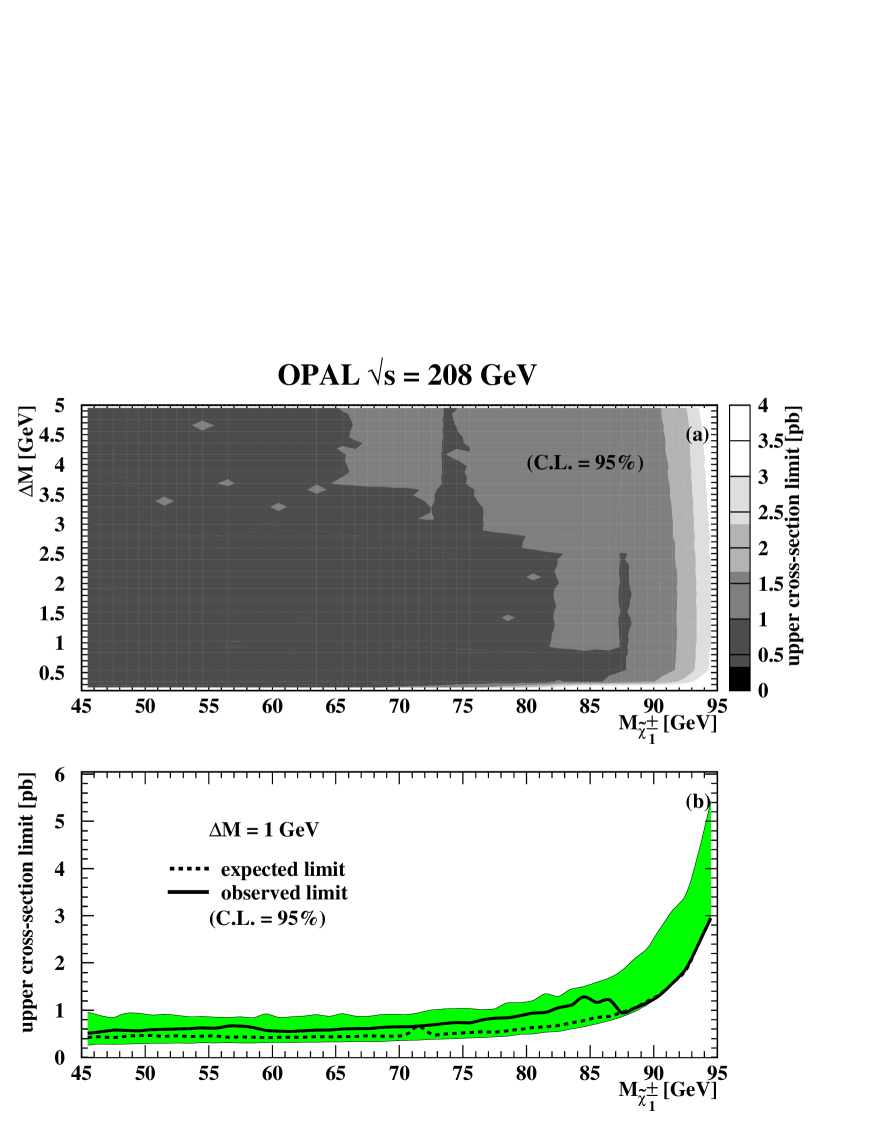
Figure 5: Upper signal cross-section limit rescaled to $\sqrt{s}=208\,\mathrm{GeV}$ at the 95% confidence level as a function of the mass difference and the chargino mass (a) and for a constant mass difference of $\Delta M=1\,\mathrm{GeV}$ (b). The band in (b) indicates the $\pm 2\sigma$ interval around the median expected value.

An upper limit for the $\tilde{\chi}^{+}_{1}$$\tilde{\chi}^{-}_{1}$ production cross-section $\sigma$ was derived from the number of expected background events, the number of observed candidates and the higgsino-like scenario signal efficiencies. The signal efficiencies of the higgsino-like scenario are slightly smaller than those of the gaugino-like scenario and therefore result in more conservative limits. Figure 5 (a) shows the observed upper cross-section limits in the ($M_{\tilde{\chi}^{\pm}_{1}}$, $\Delta M$) plane. Production cross-sections above $\sim$ 0.4 – 3.7 pb were excluded for chargino masses up to $\sim 95$ $\mathrm{GeV}$ and for $0.5\,\mathrm{GeV}\leq\Delta M\leq 5.0\,\mathrm{GeV}$ at the $95\%$ confidence level ($\mathrm{C.L.}$) rescaled to $\sqrt{s}=208\,\mathrm{GeV}$ assuming the signal cross-section evolution with $\sqrt{s}$ calculated by SUSYGEN. The expected and observed upper cross-section limits for $\Delta M$=1 $\mathrm{GeV}$ as a function of the chargino mass are illustrated in Figure 5 (b).

6.2 Interpretation within the MSSM

Within the supergravity version of the MSSM [2, 3, *Arnowitt:1997um], the chargino and neutralino masses depend on four parameters: the ratio of the two Higgs vacuum expectation values, $\tan\beta$; the Higgs mixing parameter, $\mu$ and the $U(1)$ and $SU(2)$ gaugino mass parameters, $M_{1}$ and $M_{2}$ respectively:

$$M_{\tilde{\chi}^{\pm}_{i=1,2}} = M_{\tilde{\chi}^{\pm}_{i=1,2}}(M_{2},\mu,\tan\beta),$$

$$M_{\tilde{\chi}^{0}_{i=1\dots 4}} = M_{\tilde{\chi}^{0}_{i=1\dots 4}}(M_{1},M_{2},\mu,\tan\beta).$$

Unless specified, in the following the value of $\tan\beta$ was set to 1.5. The MSSM can have small mass differences $\Delta M$ in the following two scenarios:

• If $|\mu|\ll M_{2}$, the lightest chargino $\tilde{\chi}^{\pm}_{1}$ is almost a higgsino. In this scenario the lightest chargino and neutralino are mass-degenerate ($M_{\tilde{\chi}^{\pm}_{1}}$$\sim$$M_{\tilde{\chi}^{0}_{1}}$$\simeq|\mu|$) for very large values of $M_{2}$. We call this the higgsino-like scenario.

• If $M_{2}\ll|\mu|$, the lightest chargino $\tilde{\chi}^{\pm}_{1}$ is almost a gaugino $\tilde{\mathrm{W}}^{\pm}$ with $M_{\tilde{\chi}^{\pm}_{1}}\sim M_{2}$. The mass of the lightest neutralino $\tilde{\chi}^{0}_{1}$ is given by $M_{\tilde{\chi}^{0}_{1}}\sim\min(M_{1},\,M_{2})$. Therefore small mass splittings only occur if $M_{2}<M_{1}$. If the masses of all gauginos are assumed to be identical at the grand unification scale (GUT), then the relation between $M_{1}$ and $M_{2}$ at the $\mathrm{Z}$-scale is given by:

  $$M_{1} = \tan^{2}\theta_{W}M_{2}\simeq\dfrac{1}{2}M_{2}.$$ (2)

  In this case the model does not predict a small $\Delta M$ gaugino-like scenario. In more general scenarios, Eq. (2) does not hold and can be generalised introducing an arbitrary factor $R_{\mathrm{S}}$:

  $$M_{1} = R_{\mathrm{S}}M_{2}.$$ (3)

  Some string theory motivated SUSY scenarios [39] explicitly predict $R_{\mathrm{S}}\not=\tan^{2}\theta_{W}$. For $R_{\mathrm{S}}\gtrsim 1$ the lightest chargino and neutralino are degenerate in mass with $M_{\tilde{\chi}^{\pm}_{1}}\sim M_{\tilde{\chi}^{0}_{1}}\sim M_{2}$.

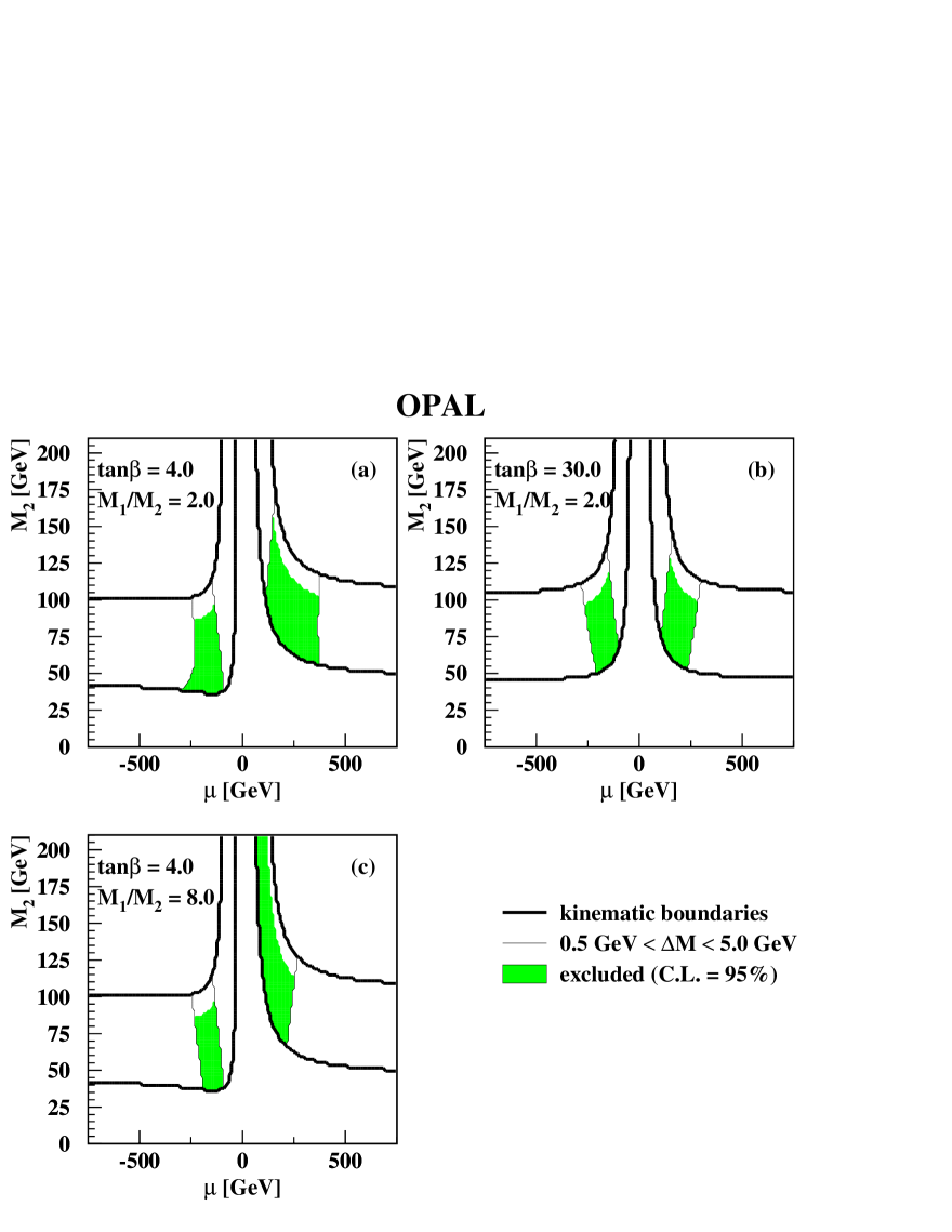
Figure 8: Exclusion regions at 95% C.L. in the $\mu$-$M_{2}$ plane within the mSUGRA framework for two values of $M_{1}/M_{2}$ and two different values of $\tan\beta$. The kinematic boundaries $(45\,\mathrm{GeV}<M_{\tilde{\chi}^{\pm}_{1}}<104\,\mathrm{GeV})$ are shown by the thick line. The thin line indicates the $\Delta M$ region considered. The shaded areas are the regions excluded by this analysis for $M_{\tilde{\chi}^{\pm}_{1}}<92\,\mathrm{GeV}$.

Figure 6 shows the cross-sections used to calculate the mass exclusion limits for the gaugino- and higgsino-scenarios. Since the coupling of the higgsino component of the chargino to the sneutrino is suppressed, the cross-sections in case of the gaugino-like scenario are more sensitive to the interfering $t$-channel production and therefore more sensitive to the sneutrino mass. The chargino mass exclusion regions for both scenarios are presented in Figure 7. From these results we derive the lower chargino mass limits listed in Table 5. The limits are valid for $0.5\,\mathrm{GeV}\leqslant\Delta M\leqslant 5.0\,\mathrm{GeV}$ and zero chargino lifetime assuming a 100% branching ratio $\tilde{\chi}^{\pm}_{1}\to\tilde{\chi}^{0}_{1}\mathrm{W}^{\pm(\star)}$. These mass limits can be directly translated into exclusion regions for the above mentioned mSUGRA parameters as shown in Figure 8.

scenario	lower $M_{\tilde{\chi}^{\pm}_{1}}$ limit (95% $\mathrm{C.L.}$)
higgsino-like	89 $\mathrm{GeV}$
gaugino-like
($M_{\tilde{\nu}}=1000\,\mathrm{GeV})$	92 $\mathrm{GeV}$
gaugino-like
($M_{\tilde{\nu}}=100\,\mathrm{GeV})$	74 $\mathrm{GeV}$

Table 5: Lower chargino mass limits at the 95% C.L. within the mSUGRA framework. The limits are valid for $0.5\,\mathrm{GeV}\leqslant\Delta M\leqslant 5.0\,\mathrm{GeV}$ and zero chargino lifetime.

6.3 Interpretation within the Anomaly Mediated SUSY Breaking Scenario

Alternatives to gravity mediated SUSY breaking scenarios can have the SUSY breaking not directly communicated from the hidden to the visible sector, as in the Anomaly Mediated SUSY Breaking Scenario (AMSB). As already mentioned in Section 1 anomalies always contribute to soft mass parameters. In AMSB gaugino masses are generated at one loop and scalar masses at two loops as a consequence of the super-Weyl anomaly [4, 5]. Here we restrict the AMSB models to those models without any further contributions from other SUSY breaking mechanisms.

In this scenario the chargino is gaugino-like and the $M_{1}/M_{2}$ ratio is $\sim 2.8$. AMSB models are described by the following parameters: a universal scalar mass at the GUT scale, $m_{0}$; the gravitino mass $m_{3/2}$; $\tan\beta$ and $\mathrm{sign}\,\mu$.

Since SUSYGEN is not able to handle AMSB scenarios, we re-interpreted our mSUGRA gaugino-like scenario results in order to give exclusion limits for the AMSB scenario. The ISAJET generator [40] was used to calculate the AMSB spectra which then were mapped to the corresponding mSUGRA cross-sections. The corresponding exclusion regions within the AMSB parameter space are shown in Figure 9.

7 Conclusions

We have searched for almost mass-degenerate charginos and neutralinos at centre-of-mass energies between 189 and 209 $\mathrm{GeV}$ with the OPAL detector at LEP. No significant excess was observed with respect to the Standard Model background. We derived a lower limit on the chargino mass of 74 $\mathrm{GeV}$ at the 95% $\mathrm{C.L.}$ for $0.5\,\mathrm{GeV}\leq\Delta M\leq 5\,\mathrm{GeV}$ in the case of light sneutrinos ($M_{\tilde{\nu}}>100\,\mathrm{GeV}$) within the mSUGRA framework. Cross-section and mass limits were translated into mSUGRA and AMSB parameter exclusion regions.

Figure 4: Absolute signal efficiency (number of selected signal events normalised to the number of generated events), $\varepsilon$, and relative efficiency (number of selected signal events normalised to a subset of generated events with $E_{\mathrm{T}}^{\gamma}>0.025\sqrt{s}$ and $|\cos\theta^{\gamma}|<0.985$), $\varepsilon^{\prime}$, at $\sqrt{s}=208\,\mathrm{GeV}$ for a constant mass difference $\Delta M=1\,\mathrm{GeV}$ ((a)+(c)) and for a constant chargino mass $M_{\tilde{\chi}^{\pm}_{1}}=80\,\mathrm{GeV}$ ((b)+(d)). The efficiencies for the gaugino-like scenario are indicated by the points. The circles correspond to the efficiencies in the case of a higgsino-like chargino.

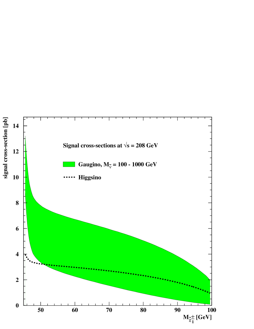
Figure 6: Signal cross-sections as a function of the chargino mass at $\sqrt{s}=208\,\mathrm{GeV}$. The shaded band shows the cross-sections in case of a gaugino-like chargino for sneutrino masses ranging from 100 to 1000 $\mathrm{GeV}$. The dashed line corresponds to the higgsino-like scenario.

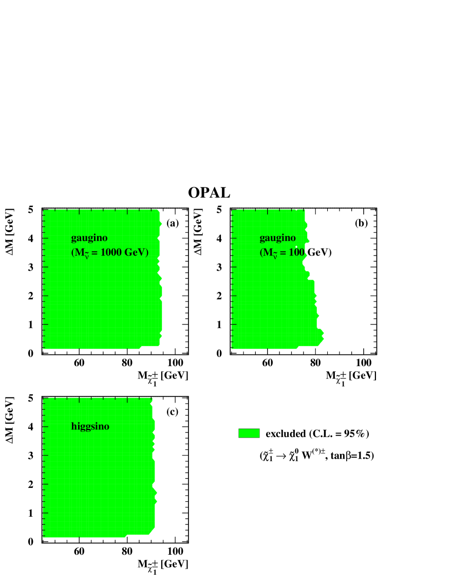
Figure 7: Lower mass limits at the 95% confidence level for various scenarios. These limits are valid for the case of a 100% branching ratio $\tilde{\chi}^{\pm}_{1}\to\tilde{\chi}^{0}_{1}\mathrm{W}^{\pm(\star)}$. The limits shown for $\Delta M<0.5\,\mathrm{GeV}$ are only valid with the assumption of a zero chargino lifetime. For the gaugino-like scenario with a light sneutrino (b) the same signal efficiencies as in the case of a heavy sneutrino (a) were assumed.

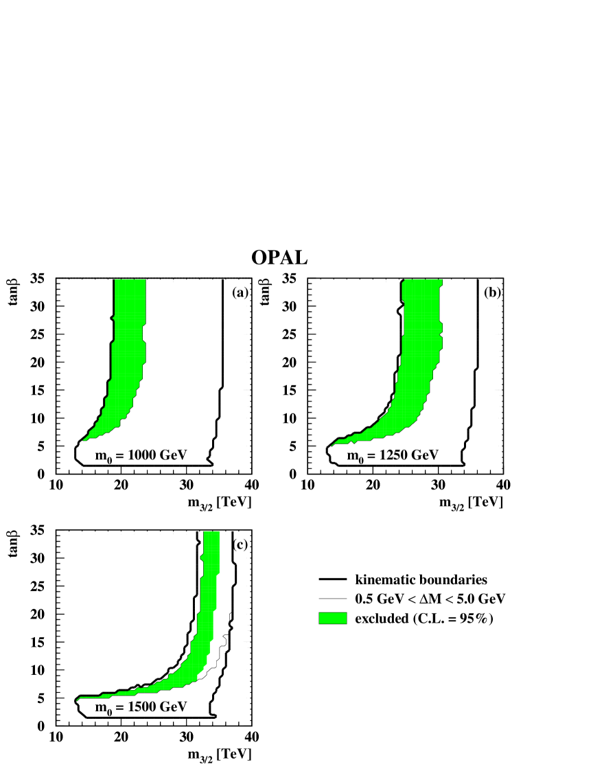
Figure 9: Exclusion regions at 95% C.L. in the $\tan\beta$-$m_{3/2}$ plane for various values of $m_{0}$ within the AMSB framework. The kinematic boundaries $(45\,\mathrm{GeV}<M_{\tilde{\chi}^{\pm}_{1}}<104\,\mathrm{GeV})$ are shown by the thick line. The region below $\tan\beta=1.5$ is theoretically inaccessible. The thin line indicates the $\Delta M$ region considered. The shaded areas are the regions excluded by this analysis.

References

-
[1]
Y.A. Golfand and E.P. Likhtman, JETP Lett. 13 (1971) 323;
D.V. Volkov and V.P. Akulov, Phys. Lett. B 46 (1973) 109;
J. Wess and B. Zumino, Nucl. Phys. B 70 (1974) 39. - [2] H.P. Nilles, Phys. Rept. 110 (1984) 1.
-
[3]
S.P. Martin, A Supersymmetry Primer, in G.L. Kane (ed.):
Perspectives On Supersymmetry, 1, hep-ph/9709356;
R. Arnowitt and P. Nath, Supergravity Unified Models, in G.L. Kane (ed.): Perspectives On Supersymmetry, 442, hep-ph/9708254. - [4] L. Randall and R. Sundrum, Nucl. Phys. B 557 (1999) 79.
- [5] G.F. Giudice, M.A. Luty, H. Murayama and R. Rattazzi, JHEP 9812 (1998) 027.
-
[6]
ALEPH Collaboration, R. Barate et al., Eur. Phys. J. C
11 (1999) 193;
ALEPH Collaboration, R. Barate et al., Eur. Phys. J. C 16 (2000) 71. -
[7]
DELPHI Collaboration, P. Abreu et al., Phys. Lett. B 479 (2000) 129;
DELPHI Collaboration, P. Abreu et al., Phys. Lett. B 503 (2001) 34. -
[8]
L3 Collaboration, M. Acciarri et al., Phys. Lett. B 472 (2000) 420;
L3 Collaboration, M. Acciarri et al., Phys. Lett. B 462 (1999) 354. -
[9]
OPAL Collaboration, G. Abbiendi et al., Eur. Phys. J. C
14 (2000) 187;
OPAL Collaboration, K. Ackerstaff et al., Phys. Lett. B 433 (1998) 195. - [10] C.H. Chen, M.Drees and J.F. Gunion, Phys. Rev. Lett. 76 (1996) 2002.
- [11] K. Riles et al., Phys. Rev. D 42 (1990) 1.
- [12] ALEPH Collaboration, A. Heister et al., Phys. Lett. B 533 (2002) 223.
- [13] DELPHI Collaboration, P. Abreu et al., Phys. Lett. B 485 (2000) 95.
- [14] L3 Collaboration, M. Acciarri et al., Phys. Lett. B 482 (2000) 31.
-
[15]
OPAL Collaboration, K. Ahmet et al., Nucl. Instrum. Meth. A 305 (1991) 275;
OPAL Collaboratio, S. Anderson et al., Nucl. Instrum. Meth. A 403 (1998) 326;
OPAL Collaboration, B. E. Anderson et al., IEEE Trans. Nucl. Sci. 41 (1994) 845. - [16] G. Aguillion et al., Nucl. Instrum. Meth. A 417 (1998) 266.
- [17] S. Katsanevas and P. Morawitz, Comput. Phys. Commun. 112 (1998) 227.
- [18] W. Beenakker et al., WW Cross-sections and Distributions, In Physics at LEP2, vol. 1, 79, hep-ph/9602351.
- [19] S. Thomas and J.D. Wells, Phys. Rev. Lett. 81 (1998) 34.
- [20] S. Jadach, B.F. Ward and Z. Was, Comput. Phys. Commun. 130 (2000) 260.
- [21] G. Montagna, M. Moretti, O. Nicrosini and F. Piccinini, Nucl. Phys. B 541 (1999) 31.
- [22] D. Karlen, Nucl. Phys. B 289 (1987) 23.
- [23] S. Jadach, W. Placzek and B.F. Ward, Phys. Lett. B 390 (1997) 298.
- [24] F.A. Berends and R. Kleiss, Nucl. Phys. B 186 (1981) 22.
-
[25]
M. Skrzypek, S. Jadach, W. Placzek and Z. Was, Comput. Phys. Commun. 94 (1996) 216;
M. Skrzypek, S. Jadach, M. Martinez, W. Placzek and Z. Was, Phys. Lett. B 372 (1996) 289. - [26] J. Fujimoto et al., Comput. Phys. Commun. 100 (1997) 128.
-
[27]
R. Engel, Z. Phys. C 66 (1995) 203;
R. Engel, J. Ranft and S. Roesler, Phys. Rev. D 52 (1995) 1459;
R. Engel and J. Ranft, Phys. Rev. D 54 (1996) 4244. - [28] G. Marchesini, B.R. Webber, G. Abbiendi, I.G. Knowles, M.H. Seymour and L. Stanco, Comput. Phys. Commun. 67 (1992) 465.
- [29] J.A.M. Vermaseren, Nucl. Phys. B 229 (1983) 347.
-
[30]
F.A. Berends, P.H. Daverveldt and R. Kleiss, Nucl. Phys. B 253 (1985) 421;
F.A. Berends, P.H. Daverveldt and R. Kleiss, Comput. Phys. Commun. 40 (1986) 271;
F.A. Berends, P.H. Daverveldt and R. Kleiss, Comput. Phys. Commun. 40 (1986) 285;
F.A. Berends, P.H. Daverveldt and R. Kleiss, Comput. Phys. Commun. 40 (1986) 309. - [31] T. Sjostrand, Comput. Phys. Commun. 39 (1986) 347.
- [32] OPAL Collaboration, J. Allison et al., Nucl. Instrum. Meth. A 317 (1992) 47.
- [33] J.F. Gunion and S. Mrenna, Phys. Rev. D 64 (2001) 075002.
- [34] OPAL Collaboration, G. Abbiendi et al., Eur. Phys. J. C 16 (2000) 185.
- [35] OPAL Collaboration, K. Ackerstaff et al., Eur. Phys. J. C 2 (1998) 213.
-
[36]
OPAL Collaboration, K. Ackerstaff et al., Phys. Lett. B
437 (1998) 218;
OPAL Collaboration, G. Abbiendi et al., Phys. Lett. B 471 (1999) 293. - [37] G. Abbiendi et al. [OPAL Collaboration], Eur. Phys. J. C 18 (2000) 253.
- [38] T. Junk, Nucl. Instrum. Meth. A 434 (1999) 435.
- [39] C.H. Chen, M. Drees and J.F. Gunion, Phys. Rev. D 55 (1997) 330.
- [40] H. Baer, F.E. Paige, S.D. Protopopescu and X. Tata, ISAJET 7.48: A Monte Carlo Event Generator for p p, anti-p p, and Reactions, (1999), hep-ph/0001086.