EUROPEAN ORGANIZATION FOR NUCLEAR RESEARCH

CERN-EP/2002-057

15th July, 2002

Charged Particle Momentum Spectra in $\mathrm{e^{+}e^{-}}$ Annihilation at $\sqrt{s}~{}=~{}192-209$ GeV

The OPAL Collaboration

Abstract

Charged particle momentum distributions are studied in the reaction $\mathrm{e^{+}e^{-}}$ $\rightarrow$ hadrons, using data collected with the OPAL detector at centre-of-mass energies from 192 GeV to 209 GeV. The data correspond to an average centre-of-mass energy of 201.7 GeV and a total integrated luminosity of 433 $\mathrm{pb}^{-1}$. The measured distributions and derived quantities, in combination with corresponding results obtained at lower centre-of-mass energies, are compared to QCD predictions in various theoretical approaches to study the energy dependence of the strong interaction and to test QCD as the theory describing it. In general, a good agreement is found between the measurements and the corresponding QCD predictions.

Submitted to Eur. Phys. J.

The OPAL Collaboration

G. Abbiendi², C. Ainsley⁵, P.F. Åkesson³, G. Alexander²², J. Allison¹⁶, P. Amaral⁹, G. Anagnostou¹, K.J. Anderson⁹, S. Arcelli², S. Asai²³, D. Axen²⁷, G. Azuelos^18,a, I. Bailey²⁶, E. Barberio⁸, R.J. Barlow¹⁶, R.J. Batley⁵, P. Bechtle²⁵, T. Behnke²⁵, K.W. Bell²⁰, P.J. Bell¹, G. Bella²², A. Bellerive⁶, G. Benelli⁴, S. Bethke³², O. Biebel³¹, I.J. Bloodworth¹, O. Boeriu¹⁰, P. Bock¹¹, D. Bonacorsi², M. Boutemeur³¹, S. Braibant⁸, L. Brigliadori², R.M. Brown²⁰, K. Buesser²⁵, H.J. Burckhart⁸, S. Campana⁴, R.K. Carnegie⁶, B. Caron²⁸, A.A. Carter¹³, J.R. Carter⁵, C.Y. Chang¹⁷, D.G. Charlton^1,b, A. Csilling^8,g, M. Cuffiani², S. Dado²¹, G.M. Dallavalle², S. Dallison¹⁶, A. De Roeck⁸, E.A. De Wolf⁸, K. Desch²⁵, B. Dienes³⁰, M. Donkers⁶, J. Dubbert³¹, E. Duchovni²⁴, G. Duckeck³¹, I.P. Duerdoth¹⁶, E. Elfgren¹⁸, E. Etzion²², F. Fabbri², L. Feld¹⁰, P. Ferrari⁸, F. Fiedler³¹, I. Fleck¹⁰, M. Ford⁵, A. Frey⁸, A. Fürtjes⁸, P. Gagnon¹², J.W. Gary⁴, G. Gaycken²⁵, C. Geich-Gimbel³, G. Giacomelli², P. Giacomelli², M. Giunta⁴, J. Goldberg²¹, E. Gross²⁴, J. Grunhaus²², M. Gruwé⁸, P.O. Günther³, A. Gupta⁹, C. Hajdu²⁹, M. Hamann²⁵, G.G. Hanson⁴, K. Harder²⁵, A. Harel²¹, M. Harin-Dirac⁴, M. Hauschild⁸, J. Hauschildt²⁵, C.M. Hawkes¹, R. Hawkings⁸, R.J. Hemingway⁶, C. Hensel²⁵, G. Herten¹⁰, R.D. Heuer²⁵, J.C. Hill⁵, K. Hoffman⁹, R.J. Homer¹, D. Horváth^29,c, R. Howard²⁷, P. Hüntemeyer²⁵, P. Igo-Kemenes¹¹, K. Ishii²³, H. Jeremie¹⁸, P. Jovanovic¹, T.R. Junk⁶, N. Kanaya²⁶, J. Kanzaki²³, G. Karapetian¹⁸, D. Karlen⁶, V. Kartvelishvili¹⁶, K. Kawagoe²³, T. Kawamoto²³, R.K. Keeler²⁶, R.G. Kellogg¹⁷, B.W. Kennedy²⁰, D.H. Kim¹⁹, K. Klein¹¹, A. Klier²⁴, S. Kluth³², T. Kobayashi²³, M. Kobel³, S. Komamiya²³, L. Kormos²⁶, R.V. Kowalewski²⁶, T. Krämer²⁵, T. Kress⁴, P. Krieger^6,l, J. von Krogh¹¹, D. Krop¹², K. Kruger⁸, M. Kupper²⁴, G.D. Lafferty¹⁶, H. Landsman²¹, D. Lanske¹⁴, J.G. Layter⁴, A. Leins³¹, D. Lellouch²⁴, J. Letts¹², L. Levinson²⁴, J. Lillich¹⁰, S.L. Lloyd¹³, F.K. Loebinger¹⁶, J. Lu²⁷, J. Ludwig¹⁰, A. Macpherson^28,i, W. Mader³, S. Marcellini², T.E. Marchant¹⁶, A.J. Martin¹³, J.P. Martin¹⁸, G. Masetti², T. Mashimo²³, P. Mättig^m, W.J. McDonald²⁸, J. McKenna²⁷, T.J. McMahon¹, R.A. McPherson²⁶, F. Meijers⁸, P. Mendez-Lorenzo³¹, W. Menges²⁵, F.S. Merritt⁹, H. Mes^6,a, A. Michelini², S. Mihara²³, G. Mikenberg²⁴, D.J. Miller¹⁵, S. Moed²¹, W. Mohr¹⁰, T. Mori²³, A. Mutter¹⁰, K. Nagai¹³, I. Nakamura²³, H.A. Neal³³, R. Nisius³², S.W. O’Neale¹, A. Oh⁸, A. Okpara¹¹, M.J. Oreglia⁹, S. Orito²³, C. Pahl³², G. Pásztor^4,g, J.R. Pater¹⁶, G.N. Patrick²⁰, J.E. Pilcher⁹, J. Pinfold²⁸, D.E. Plane⁸, B. Poli², J. Polok⁸, O. Pooth¹⁴, M. Przybycień^8,n, A. Quadt³, K. Rabbertz⁸, C. Rembser⁸, P. Renkel²⁴, H. Rick⁴, J.M. Roney²⁶, S. Rosati³, Y. Rozen²¹, K. Runge¹⁰, K. Sachs⁶, T. Saeki²³, O. Sahr³¹, E.K.G. Sarkisyan^8,j, A.D. Schaile³¹, O. Schaile³¹, P. Scharff-Hansen⁸, J. Schieck³², T. Schörner-Sadenius⁸, M. Schröder⁸, M. Schumacher³, C. Schwick⁸, W.G. Scott²⁰, R. Seuster^14,f, T.G. Shears^8,h, B.C. Shen⁴, C.H. Shepherd-Themistocleous⁵, P. Sherwood¹⁵, G. Siroli², A. Skuja¹⁷, A.M. Smith⁸, R. Sobie²⁶, S. Söldner-Rembold^10,d, S. Spagnolo²⁰, F. Spano⁹, A. Stahl³, K. Stephens¹⁶, D. Strom¹⁹, R. Ströhmer³¹, S. Tarem²¹, M. Tasevsky⁸, R.J. Taylor¹⁵, R. Teuscher⁹, M.A. Thomson⁵, E. Torrence¹⁹, D. Toya²³, P. Tran⁴, T. Trefzger³¹, A. Tricoli², I. Trigger⁸, Z. Trócsányi^30,e, E. Tsur²², M.F. Turner-Watson¹, I. Ueda²³, B. Ujvári^30,e, B. Vachon²⁶, C.F. Vollmer³¹, P. Vannerem¹⁰, M. Verzocchi¹⁷, H. Voss⁸, J. Vossebeld^8,h, D. Waller⁶, C.P. Ward⁵, D.R. Ward⁵, P.M. Watkins¹, A.T. Watson¹, N.K. Watson¹, P.S. Wells⁸, T. Wengler⁸, N. Wermes³, D. Wetterling¹¹ G.W. Wilson^16,k, J.A. Wilson¹, G. Wolf²⁴, T.R. Wyatt¹⁶, S. Yamashita²³, D. Zer-Zion⁴, L. Zivkovic²⁴

¹School of Physics and Astronomy, University of Birmingham, Birmingham B15 2TT, UK
²Dipartimento di Fisica dell’ Università di Bologna and INFN, I-40126 Bologna, Italy
³Physikalisches Institut, Universität Bonn, D-53115 Bonn, Germany
⁴Department of Physics, University of California, Riverside CA 92521, USA
⁵Cavendish Laboratory, Cambridge CB3 0HE, UK
⁶Ottawa-Carleton Institute for Physics, Department of Physics, Carleton University, Ottawa, Ontario K1S 5B6, Canada
⁸CERN, European Organisation for Nuclear Research, CH-1211 Geneva 23, Switzerland
⁹Enrico Fermi Institute and Department of Physics, University of Chicago, Chicago IL 60637, USA
¹⁰Fakultät für Physik, Albert-Ludwigs-Universität Freiburg, D-79104 Freiburg, Germany
¹¹Physikalisches Institut, Universität Heidelberg, D-69120 Heidelberg, Germany
¹²Indiana University, Department of Physics, Swain Hall West 117, Bloomington IN 47405, USA
¹³Queen Mary and Westfield College, University of London, London E1 4NS, UK
¹⁴Technische Hochschule Aachen, III Physikalisches Institut, Sommerfeldstrasse 26-28, D-52056 Aachen, Germany
¹⁵University College London, London WC1E 6BT, UK
¹⁶Department of Physics, Schuster Laboratory, The University, Manchester M13 9PL, UK
¹⁷Department of Physics, University of Maryland, College Park, MD 20742, USA
¹⁸Laboratoire de Physique Nucléaire, Université de Montréal, Montréal, Quebec H3C 3J7, Canada
¹⁹University of Oregon, Department of Physics, Eugene OR 97403, USA
²⁰CLRC Rutherford Appleton Laboratory, Chilton, Didcot, Oxfordshire OX11 0QX, UK
²¹Department of Physics, Technion-Israel Institute of Technology, Haifa 32000, Israel
²²Department of Physics and Astronomy, Tel Aviv University, Tel Aviv 69978, Israel
²³International Centre for Elementary Particle Physics and Department of Physics, University of Tokyo, Tokyo 113-0033, and Kobe University, Kobe 657-8501, Japan
²⁴Particle Physics Department, Weizmann Institute of Science, Rehovot 76100, Israel
²⁵Universität Hamburg/DESY, Institut für Experimentalphysik, Notkestrasse 85, D-22607 Hamburg, Germany
²⁶University of Victoria, Department of Physics, P O Box 3055, Victoria BC V8W 3P6, Canada
²⁷University of British Columbia, Department of Physics, Vancouver BC V6T 1Z1, Canada
²⁸University of Alberta, Department of Physics, Edmonton AB T6G 2J1, Canada
²⁹Research Institute for Particle and Nuclear Physics, H-1525 Budapest, P O Box 49, Hungary
³⁰Institute of Nuclear Research, H-4001 Debrecen, P O Box 51, Hungary
³¹Ludwig-Maximilians-Universität München, Sektion Physik, Am Coulombwall 1, D-85748 Garching, Germany
³²Max-Planck-Institute für Physik, Föhringer Ring 6, D-80805 München, Germany
³³Yale University, Department of Physics, New Haven, CT 06520, USA

^a and at TRIUMF, Vancouver, Canada V6T 2A3
^b and Royal Society University Research Fellow
^c and Institute of Nuclear Research, Debrecen, Hungary
^d and Heisenberg Fellow
^e and Department of Experimental Physics, Lajos Kossuth University, Debrecen, Hungary
^f and MPI München
^g and Research Institute for Particle and Nuclear Physics, Budapest, Hungary
^h now at University of Liverpool, Dept of Physics, Liverpool L69 3BX, UK
ⁱ and CERN, EP Div, 1211 Geneva 23
^j and Universitaire Instelling Antwerpen, Physics Department, B-2610 Antwerpen, Belgium
^k now at University of Kansas, Dept of Physics and Astronomy, Lawrence, KS 66045, USA
^l now at University of Toronto, Dept of Physics, Toronto, Canada
^m current address Bergische Universität, Wuppertal, Germany
ⁿ and University of Mining and Metallurgy, Cracow, Poland

1 Introduction

Charged particle momentum distributions are studied in the hadronic decays of virtual photons or Z bosons (hereafter referred to as $(\mathrm{Z}/\gamma)^{*}$ decays) at centre-of-mass (c.m.) energies, $\sqrt{s}$, between 192 and 209 GeV, the highest available $\mathrm{e^{+}e^{-}}$ energies. These distributions can be measured with relatively high precision. Combined with lower energy data they provide a powerful test of quantum chromodynamics (QCD) as the theory describing the strong interaction.

Previous studies using $\mathrm{e^{+}e^{-}}$ annihilation data at c.m. energies from 130 up to 189 GeV have shown that QCD based models and calculations give a good description of most of the measured distributions [1, 2, 3, 4, 5, 6]. With the yet higher energy data used in this paper, we obtain even more stringent tests of the models and theory. In addition we use these highest energy data in combination with earlier measurements at lower c.m. energies to study the energy dependence of the strong interaction.

We measure the charged particle momentum distribution, $1/\sigma\cdot\mathrm{d}\sigma_{\mathrm{ch}}/\mathrm{d}x_{p}$, and the $\xi_{p}$ distribution, $1/\sigma\cdot\mathrm{d}\sigma_{\mathrm{ch}}/\mathrm{d}\xi_{p}$, where $x_{p}=2p/\sqrt{s}$, $\xi_{p}=\ln(1/x_{p})$, $p$ is the particle momentum, $\sigma$ is the cross-section for non-radiative hadronic $(\mathrm{Z}/\gamma)^{*}$ decays and $\sigma_{\mathrm{ch}}$ is the charged particle cross-section in these events. We also measure the distribution of the rapidity, $y=\frac{1}{2}\left|\ln\left({{E+p_{\|}}\over{E-p_{\|}}}\right)\right|$, where $p_{\|}$ is the momentum component parallel to the thrust axis and $E$ is the energy of the particle, and the distributions of the 3-momentum components in, $p_{\perp}^{\mathrm{in}}$, and perpendicular to, $p_{\perp}^{\mathrm{out}}$, the event plane. This plane is defined by the eigenvectors associated with the two largest eigenvalues of the momentum tensor, as in reference [1].

We present comparisons of the fractional momentum distributions $1/\sigma\cdot\mathrm{d}\sigma_{\mathrm{ch}}/\mathrm{d}x_{p}$ and $1/\sigma\cdot\mathrm{d}\sigma_{\mathrm{ch}}/\mathrm{d}\xi_{p}$ in the range $\sqrt{s}=14-202$ GeV to QCD predictions in different theoretical approaches. As in earlier publications [1, 2, 3] we also study the evolution with the c.m. energy of the peak position $\xi_{0}$ in the $\xi_{p}$ distribution.

In Section 2 a brief description of the OPAL detector is given. The samples of data and simulated events used in the analysis are described in Section 3. In Section 4 the event selection and analysis procedure are described. In Section 5 we present the observed distributions and, together with those obtained at lower energies, compare them to the predictions of different Monte Carlo programs and analytic QCD predictions. A summary and conclusions are given in Section 6.

2 The OPAL detector

The OPAL detector was operated at the LEP $\mathrm{e^{+}e^{-}}$ collider at CERN. A detailed description can be found in [7]. The analysis presented here relies mainly on the measurement of momenta and directions of charged particles in the tracking chambers and of energy deposited in the electromagnetic calorimeters of the detector.

All tracking systems were located inside a solenoidal magnet which provided a uniform axial magnetic field of 0.435 T along the beam axis. The magnet was surrounded by a lead glass electromagnetic calorimeter and a hadron calorimeter of the sampling type. Outside the hadron calorimeter, the detector was surrounded by a system of muon chambers. There were similar layers of detectors in the forward and backward endcaps.

The tracking system consisted of a silicon microvertex detector, an inner vertex chamber, a large volume jet chamber, and specialised chambers at the outer radius of the jet chamber to improve the measurements in the $z$ direction. The main tracking detector was the central jet chamber. This device was approximately 4 m long and had an outer radius of about 1.85 m. It had 24 sectors with radial planes of 159 sense wires spaced by 1 cm. The momenta $p$ of tracks in the $r$-$\phi$ plane were measured with a precision $\sigma_{p}/p=\sqrt{0.02^{2}+(0.0015\cdot p[\mathrm{GeV}/c])^{2}}$.

The electromagnetic calorimeters in the barrel and the endcap sections of the detector consisted of 11704 lead glass blocks with a depth of $24.6$ radiation lengths in the barrel and typically $22$ radiation lengths in the endcaps. The barrel section covered the angular region $|\cos{\theta}|<0.82$ and the endcap section the region $0.82<|\cos{\theta}|<0.98$.

3 Data and Monte Carlo samples

The data used in this measurement were recorded in 1999 and 2000, the final two years of the LEP 2 program. During this time $\mathrm{e^{+}e^{-}}$ interactions were collected at c.m. energies in the range 192-209 GeV. The total integrated luminosity of the data sample, as evaluated using small angle Bhabha collisions, is 433 $\mathrm{pb}^{-1}$. The luminosity collected at the different c.m. energies is detailed in Figure 1 and in Table 1.

Monte Carlo event samples were generated at c.m. energies of 192, 196, 200, 202, 206 and 208 GeV and were processed using a full simulation of the OPAL detector [8]. Distributions at intermediate energies were obtained by linear interpolation between the distributions at the nearest neighbouring available c.m. energies. In general, the Monte Carlo samples contain at least 10 times the statistics of the data. Signal $\mathrm{e^{+}e^{-}}\rightarrow(\mathrm{Z}/\gamma)^{*}\rightarrow\mathrm{q\overline{q}}({\rm g})$ events were generated using the PYTHIA 6.125 [9, 10] Monte Carlo program for the parton shower and hadronisation stage, which was interfaced with the KK2F program [11] to obtain a more accurate description of initial state radiation (ISR). The simulation parameters were tuned to OPAL data taken at the $\mathrm{Z}$ peak [12]. The PYTHIA Monte Carlo model has previously been shown to provide a good description of $\mathrm{e^{+}e^{-}}$ annihilation data for c.m. energies up to 189 GeV (see e.g. [1, 2, 3, 4, 5, 6, 12]).

As an alternative to the string fragmentation model implemented in PYTHIA, events were generated using the HERWIG 5.9 [13] Monte Carlo program, also tuned to OPAL data as described in [2, 12]. The HERWIG Monte Carlo program implements the cluster fragmentation model.

In addition, we generated events of the type $\mathrm{e^{+}e^{-}}\rightarrow 4$ fermions (diagrams without intermediate gluons). These 4-fermion events, in particular those with four quarks in the final state, constitute the major background in this analysis. Simulated 4-fermion events with hadronic and leptonic final states were generated using the GRC4F 2.1 [14] Monte Carlo program. The final states were produced via $s$-channel or $t$-channel diagrams, including $\mathrm{W^{+}W^{-}}$ and $\mathrm{ZZ}$ production. This generator was interfaced to JETSET 7.4 [9] using the same parameter set [12] for the fragmentation and decays as used for $(\mathrm{Z}/\gamma)^{*}$ events. The JETSET program implements the string fragmentation model.

Two other possible sources of background events were simulated. Hadronic two-photon processes were evaluated using the VERMASEREN [15], HERWIG and PHOJET [16] programs. Production of $\mathrm{e^{+}e^{-}}\rightarrow(\mathrm{Z}/\gamma)^{*}\rightarrow\tau^{+}\tau^{-}$ was evaluated using the KK2F event generator in combination with the TAUOLA [17] decay library to simulate the decay of the tau leptons.

In addition to PYTHIA and HERWIG we also used the ARIADNE 4.08 [18] event generator to compare to our corrected data distributions. The ARIADNE program implements the colour dipole model to describe the parton shower process. For the fragmentation stage the generator was interfaced to the JETSET 7.4 program. The parameter set used for ARIADNE is documented in [19]. This model provides a good description of global $\mathrm{e^{+}e^{-}}$ event properties at $\sqrt{s}=M_{\mathrm{Z}}$, as do PYTHIA and HERWIG.

4 Data analysis

4.1 Selection of events

The majority of hadronic events produced at c.m. energies above the $\mathrm{Z}$ resonance are radiative events in which initial state photon radiation reduces the invariant mass of the hadronic system to about $M_{\mathrm{Z}}$. An experimental separation between radiative and non-radiative events is therefore required. In addition, at the present energies above 190 GeV, $\mathrm{ZZ}$ and $\mathrm{W^{+}W^{-}}$ production are kinematically possible and form a significant background to the $(\mathrm{Z}/\gamma)^{*}\rightarrow\mathrm{q\overline{q}}$ events. In this paper we use similar techniques to those of our previous analyses of $\mathrm{e^{+}e^{-}}$ annihilation data at lower c.m. energies [1, 2, 3], to select non-radiative $(\mathrm{Z}/\gamma)^{*}\rightarrow\mathrm{q\overline{q}}$ events.

4.1.1 Preselection

Hadronic events are identified using criteria as described in [20]. The efficiency of selecting non-radiative hadronic events is greater than 98% at all c.m. energies, as can be seen in Table 1. We define as particles tracks recorded in the tracking chambers and clusters recorded in the electromagnetic calorimeter. The tracks are required to have transverse momentum relative to the beam axis, $p_{T}>150$ MeV/$c$, a number of hits in the jet chamber, $N_{\rm hits}\geq 40$, a distance of the point of closest approach to the collision point in the $r$-$\phi$ plane, $d_{0}\leq 2$ cm, and along the $z$ axis, $z_{0}\leq 25$ cm. The clusters in the electromagnetic calorimeter are required to have a minimum energy of 100 MeV in the barrel and 250 MeV in the endcap sections.

4.1.2 ISR-fit selection

To reject radiative events, we determine the effective c.m. energy $\sqrt{s^{\prime}}$ of the observed hadronic system as follows [21].

First isolated photons are identified by looking for energy deposits greater than 3 GeV in the electromagnetic calorimeter, having less than 1 GeV of additional energy deposited in a cone of 0.2 radians around its direction. The remaining particles are formed into jets using the Durham [22] algorithm with a value for the resolution parameter $y_{\mathrm{cut}}=0.02$. A matching algorithm [23] is employed to reduce double counting of energy in cases where charged tracks point towards electromagnetic clusters. The energy of additional photons emitted close to the beam direction is estimated by performing three separate kinematic fits assuming zero, one or two such photons. Of the acceptable fits, the one with the lowest number of photons is selected. The value of $\sqrt{s^{\prime}}$ is computed from the fitted momenta of the jets, excluding photons identified in the detector or close to the beam directions. The value of $\sqrt{s^{\prime}}$ is set to $\sqrt{s}$ if the fit assuming zero initial state photons was selected. The 4-momenta of all measured particles are boosted into the rest frame of the observed hadronic system.

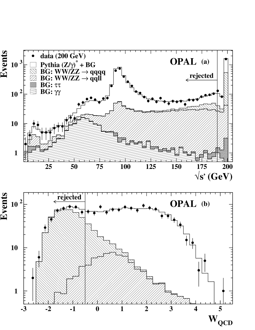
Figure 2: Distributions of (a) the effective c.m. energy $\sqrt{s^{\prime}}$ and (b) the QCD event weight $W_{\mathrm{QCD}}$ in the data at $\sqrt{s}=200$ GeV (full points). The data are shown with statistical errors only. Estimated signal and background (BG) contributions are shown as detailed in the upper figure. The vertical lines indicate where the selection cuts are applied.

To reject events with large initial-state radiation (ISR), we require $\sqrt{s^{\prime}}>\sqrt{s}-10$ GeV. This is referred to as the “ISR-fit” selection. In Figure 2a we compare the $\sqrt{s^{\prime}}$ distribution of the data set at $\sqrt{s}$=200 GeV, after the preselection was applied, to simulated $(\mathrm{Z}/\gamma)^{*}$ events and to 4-fermion and other background events. Simulated $(\mathrm{Z}/\gamma)^{*}$ events are classified into radiative events, $\sqrt{s^{\prime}_{\mathrm{true}}}<\sqrt{s}-1$ GeV, where $\sqrt{s^{\prime}_{\mathrm{true}}}$ is the true effective c.m. energy, and non-radiative events, which is the complement. Though about 27% of the selected $(\mathrm{Z}/\gamma)^{*}$ events are by this definition radiative events, the fraction of selected events with $\sqrt{s^{\prime}_{\mathrm{true}}}<\sqrt{s}-10$ GeV is only 5%. The background from 4-fermion events and the efficiency of selecting non-radiative events are given in Table 1.

4.1.3 Final selection

The estimated background from $\mathrm{e^{+}e^{-}}\rightarrow\tau^{+}\tau^{-}$ and two-photon events of the type $\gamma\gamma\rightarrow\mathrm{q\overline{q}}$ is small at high $\sqrt{s^{\prime}}$. To reject this background further and to ensure events are well contained in the OPAL detector we require at least seven accepted tracks, and the cosine of the polar angle of the thrust axis, $|\cos\theta_{T}|<0.9$. The background from the $\tau^{+}\tau^{-}$ and two-photon events in the final selected sample is estimated from Monte Carlo samples to be about 0.1% and is neglected.

To reduce the background of 4-fermion events in the remaining sample, we test the compatibility of the events with QCD-like production processes. A QCD event weight $W_{\mathrm{QCD}}$ is computed as follows. We force each event into a four-jet configuration in the Durham jet scheme and use the EVENT2 [24] program to calculate the $\mathcal{O}(\alpha_{s}^{2})$ matrix element $\left|{\cal M}(p_{1},p_{2},p_{3},p_{4})\right|^{2}$ for the processes $\mathrm{e^{+}e^{-}}\rightarrow\mathrm{q\bar{q}q\bar{q},q\bar{q}gg}$ [25], where $p_{1}$, $p_{2}$, $p_{3}$ and $p_{4}$ are the momenta of the reconstructed jets. Since neither quark nor gluon identification is performed on the jets, we calculate the matrix element for each permutation of the jet momenta and use the permutation with the largest value for the matrix element to define the event weight,

$$W_{\mathrm{QCD}}=\max_{\left\{p_{1},p_{2},p_{3},p_{4}\right\}}\log\left(\left|{\cal M}(p_{1},p_{2},p_{3},p_{4})\right|^{2}\right).$$ (1)

Note that the definition of the event weight contains kinematic information only and is independent of the value of $\alpha_{s}$.

The weight $W_{\mathrm{QCD}}$ is expected to have large values for processes described by the QCD matrix element, originating from $(\mathrm{Z}/\gamma)^{*}\rightarrow\mathrm{q\overline{q}}$, and smaller values for $\mathrm{W^{+}W^{-}}$ or $\mathrm{ZZ}$ events. In Figure 2b we compare the data distribution of $W_{\mathrm{QCD}}$, after the ISR-fit selection, to the expectations of our simulation. A good separation between the $(\mathrm{Z}/\gamma)^{*}$ and 4-fermion events is achieved by requiring $W_{\mathrm{QCD}}\geq-0.5$.

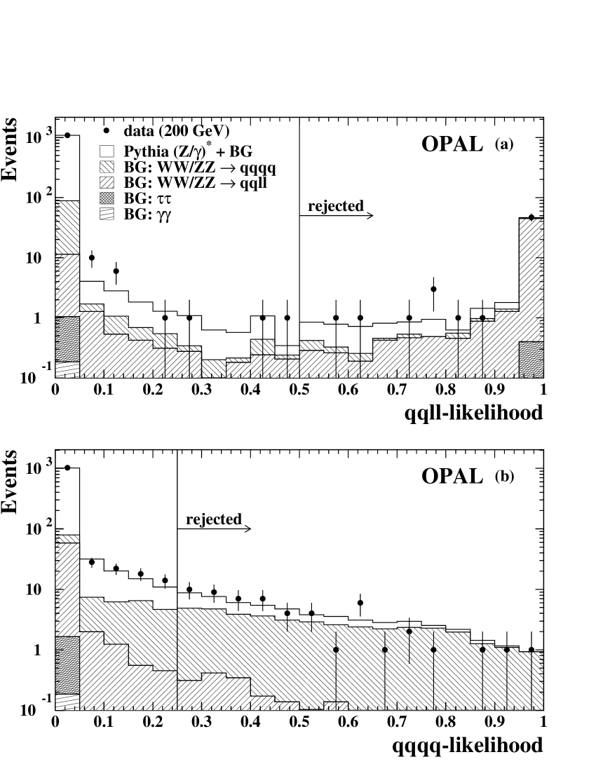
Figure 3: Distributions of the likelihood for events to be (a) a semi-leptonic 4-fermion event or (b) a hadronic 4-fermion event, in the data at $\sqrt{s}=200$ GeV (full points). The data are shown with statistical errors only. Estimated signal and background (BG) contributions are shown as detailed in the upper figure. The vertical lines indicate where the selection cuts are applied.

In addition to the cut on $W_{\mathrm{QCD}}$, used also in our earlier papers, we apply a likelihood based rejection of hadronic and semi-leptonic $\mathrm{ZZ}$ and $\mathrm{W^{+}W^{-}}$ decays (see [26] and references therein). The distributions for the semi-leptonic and hadronic likelihoods, after all selection cuts described above, are shown in Figure 3a and 3b, for the data and for the signal and background Monte Carlo expectations. Events are rejected if the semi-leptonic likelihood is greater than 0.5 or the hadronic likelihood is greater than 0.25, thus reducing the remaining 4-fermion background by more than a factor two while reducing the expected signal by only about 2.2%. After the final selection criteria the estimated efficiency for selecting signal events is around 76% while the remaining 4-fermion background in estimated to be around 5%. The individual numbers for each of the six energy ranges are given Table 1.

4.2 Correction procedure

The remaining 4-fermion background in each bin of each observable was estimated by Monte Carlo simulation and is subtracted from the observed bin content. A bin-by-bin multiplication procedure is then used to correct the observed distributions for the effects of detector resolution and acceptance as well as for the presence of remaining radiative $(\mathrm{Z}/\gamma)^{*}$ events. A bin-by-bin correction procedure is suitable for the measured distributions as the effects of finite resolution and acceptance cause only limited migration (and therefore correlation) between bins and the data are well described by the Monte Carlo programs used to determine the corrections.

For the multiplicative correction each bin, after background subtraction, is corrected from the “detector level” to the “hadron level” using two samples of Monte Carlo $(\mathrm{Z}/\gamma)^{*}$ events at each c.m. energy. The hadron level sample does not include initial state radiation or detector effects and allows all particles with lifetimes shorter than $3\times 10^{-10}$ s to decay. The detector level sample includes full simulation of the OPAL detector and initial state radiation and contains only those events which pass the same cuts as are applied to the data. The bin-by-bin correction factors are derived from the ratio of the distributions at the hadron level to those at the detector level. The correction factors tend to be around 1.15 in most bins, with values further away from 1 at the edges of the distributions.

4.3 Systematic uncertainties

The experimental systematic uncertainties are estimated by repeating the analysis with varied experimental conditions. To reduce statistical fluctuations in the magnitudes of the systematic uncertainties the average over three neighbouring bins is taken. In addition, all results and errors obtained for the different energy ranges are combined in a single set of results, as described in Section 4.4, thus further reducing any statistical fluctuations in the systematic uncertainties.

Possible inadequacies in the simulation of the response of the detector in the endcap regions are accounted for by restricting the analysis to the barrel region of the detector, requiring the thrust axis of accepted events to lie within the range $|\cos\theta_{T}|<0.7$. This reduces the event sample by approximately 26%. The corresponding systematic error is the deviation of the results from those of the standard analysis.

To evaluate uncertainties due to inadequacies in the track modelling the selection criteria for tracks were modified. The maximum allowed distance of the point of closest approach of a track to the collision point in the $r$-$\phi$ plane, $d_{0}$, was changed from 2 to 5 cm, the maximum distance in the $z$ direction, $z_{0}$, from 25 to 10 cm and the minimum number of hits from 40 to 80. These modifications change the number of selected tracks by up to approximately 12%. In addition, track momenta in the Monte Carlo samples were smeared to degrade the resolution by 10%. The quadratic sum over the deviations from the standard result, obtained from each of these variations, is included in the total systematic uncertainty.

Uncertainties arising from the selection of non-radiative events are estimated by repeating the analysis using a different technique[2] to determine the value for $\sqrt{s^{\prime}}$. This technique differs from our standard $\sqrt{s^{\prime}}$ algorithm in that in this case the kinematic fit always assumes one photon, either unobserved close to the beam direction, or detected in the ECAL. The final event sample with this $\sqrt{s^{\prime}}$ algorithm has an overlap of approximately 97% with the standard sample and is approximately the same size. The difference relative to the standard result is included in the total systematic error.

Systematic uncertainties associated with the subtraction of the 4-fermion background events are estimated by varying the cut on $W_{\mathrm{QCD}}$ and on the 4-fermion likelihoods. We use $W_{\mathrm{QCD}}\geq-0.8$ which increases the event sample by approximately 2%, and $W_{\mathrm{QCD}}\geq 0$ which reduces the event sample by approximately 8%. We also vary the cuts on the likelihood values between 0.1 and 0.4 for hadronic 4-fermion events and between 0.25 and 0.75 for semi-leptonic events. The maximum deviation from the standard result obtained from the variations of the cuts on $W_{\mathrm{QCD}}$ and the hadronic 4-fermion likelihood is included in the total systematic uncertainty, as is the maximum deviation obtained from the variations of the cut on the semi-leptonic likelihood.

In addition, we vary the predicted background to be subtracted, up and down by 5%, slightly more than its measured uncertainty at $\sqrt{s}$= 189 GeV of 4% [26], and include the largest difference from the standard result in the systematic uncertainty.

The difference in the results when we determine the bin-to-bin correction factors from simulated $(\mathrm{Z}/\gamma)^{*}$ events generated using HERWIG instead of PYTHIA is taken as the uncertainty in the modelling of the $(\mathrm{Z}/\gamma)^{*}$ events.

All systematic uncertainties are added in quadrature to obtain the total systematic errors. The largest contribution to the total uncertainty is that obtained using HERWIG as an alternative hadronisation model in the correction procedure. Other significant contributions to the systematic uncertainties arise from varying the quality criteria on tracks and from varying the 4-fermion rejection cuts.

4.4 Combining results

The event selection, the correction procedure and the estimate of systematic uncertainties are performed independently for each of the six energy regions detailed in Table 1. Afterwards the results are combined to obtain a single set of results with the best possible statistical precision. The combination procedure assumes all systematic uncertainties to be fully correlated between the energy regions. This means data points obtained at different energies are combined into a weighted average, using the statistical errors to determine the weights.

To obtain the systematic uncertainty on the combined results all individual contributions to the systematic uncertainty, described in Section 4.3, are first determined separately in each energy region. For the combined results the individual contributions to the systematic uncertainty are then taken as the average over the corresponding values obtained in each of the six energy regions. Finally, the combination of the thus averaged individual contributions into the total systematic uncertainty on the combined results is done, as in Section 4.3, by adding all contributions in quadrature.

5 Results and comparison to theory

The $p_{\perp}^{\mathrm{in}}$, $p_{\perp}^{\mathrm{out}}$, $y$, $x_{p}$ and $\xi_{p}$ distributions, averaged over the full c.m. energy range $\sqrt{s}~{}=~{}192-209$ GeV, are tabulated in Tables 2 to 6 and shown in Figures 4 and 5. These distributions correspond to an average c.m. energy of $\langle\sqrt{s}\,\rangle=201.7$ GeV with a standard deviation of 4.8 GeV. They are compared to the corresponding predictions of the PYTHIA, HERWIG and ARIADNE Monte Carlo programs. In general, a reasonable agreement is observed between the predictions and the data for the different distributions. The HERWIG Monte Carlo program agrees better with the data than the PYTHIA and ARIADNE models. The $p_{\perp}^{\mathrm{out}}$ distribution is harder in the data than predicted by any of the Monte Carlo programs.

There are different theoretical approaches in which fractional energy spectra of final state hadrons can be calculated. At high $x$, conventional perturbation theory, utilising expansions in powers of $\alpha_{s}$, is applicable. Non-perturbative effects occurring at the final stage of the hadronisation process are not calculable but they can be factorised out and left to be determined experimentally. At low $x$, perturbation theory can also be applied, provided that logarithmically enhanced terms (e.g. $\sim\ln(1/x)$) are resummed to all orders. Remaining singular effects are not accounted for and as a consequence the predictions obtained are formally only valid for asymptotically high energies. Corrections to these asymptotic predictions can be calculated as an expansion in powers of $\sqrt{\alpha_{s}}$. An important precondition to the validity of these asymptotic predictions is that the non-perturbative hadron formation process is local, i.e. the properties of the hadronic final state closely follow the properties of the partons before hadronisation. This presumed equivalence is referred to as Local Parton-Hadron Duality (LPHD) [27]. For a recent review of particle production in the low $x$ region we refer to [28].

In the following, we compare $x_{p}$ and $\xi_{p}$ distributions over a large range of c.m. energies to theoretical predictions applicable to either the low $x$ or high $x$ regions, in order to test the validity of these QCD approaches and the LPHD hypothesis. Since the ranges in $x_{p}$ or $\xi_{p}$ over which the different predictions are valid depend not only on the terms included in these predictions, but also on those that are missing, we do not quantitatively know these ranges a priori. Our approach, therefore, is to fit predictions to the data in a range where they can be observed to describe the data well. We subsequently vary these ranges and extrapolate the fitted predictions outside them to establish the limits of the validity of the predictions.

5.1 Comparisons to theory at low $x$

5.1.1 Fong and Webber prediction

At low $x$, QCD predicts destructive interference effects in soft gluon emissions, causing the asymptotic shape of the $\xi$ distribution to be Gaussian [29]. The position of the peak in the distribution is predicted to increase linearly with $\tau=\ln{(\sqrt{s}/2\Lambda)}$, where $\Lambda$ is the QCD scale, defined using the one loop expression: $\alpha_{s}(\tau)=2\pi/\beta\tau$, with $\beta=11-2N_{f}/N_{c}$, $N_{c}$ the number of colours and $N_{f}$ the number of active flavours. Corrections to this asymptotic prediction were calculated up to $\mathcal{O}(\alpha_{s})$ by Fong and Webber [30], yielding a skewed Gaussian shape for the $\xi$ spectrum:

$$F_{q}(\xi,\tau)={N(\tau)\over\sigma\sqrt{2\pi}}\exp\left({k\over 8}-{s\delta\over 2}-{(2+k)\delta^{2}\over 4}+{s\delta^{3}\over 6}+{k\delta^{4}\over 24}\right),$$ (2)

where $\delta=(\xi-\bar{\xi})/\sigma$ and, for quark initiated jets:

$$\bar{\xi} = {\tau\over 2}\left(1+{\rho\over 24}\sqrt{48\over\beta\tau}\right)\left(1-{\omega\over 6\tau}\right)+\bar{\xi}_{0}\,,$$ (3)

$$\sigma = \sqrt{\tau\over 3}\left({\beta\tau\over 48}\right)^{1\over 4}\left(1-{\beta\over 64}\sqrt{48\over\beta\tau}\right)\left(1+{\omega\over 8\tau}\right)\,,$$ (4)

$$s = -{\rho\over 16}\sqrt{3\over\tau}\left({48\over\beta\tau}\right)^{1\over 4}\left(1-{3\omega\over 8\tau}\right)\,,$$ (5)

$$k = -{27\over 5\tau}\left(\sqrt{\beta\tau\over 48}-{\beta\over 24}\right)\left(1-{\omega\over 12\tau}\right)\,,$$ (6)

with $\rho=11+2N_{f}/N_{c}^{3}\,$ and $\omega=1+N_{f}/N_{c}^{3}$. The term $\bar{\xi_{0}}$ is a non-perturbative offset to the $\xi$ distribution.

We have fitted Equation (2) simultaneously to the $\xi_{p}$ distribution measured in the present study and in previous studies by OPAL [31, 1, 2, 3] and lower energy experiments [32, 33], covering the range $\sqrt{s}=14-202$ GeV. As the energy scale involved in coherent parton emissions, as described by the formalism, is expected to be low, we apply the formalism assuming three active flavours. The free parameters in the prediction are $\Lambda$ and $\bar{\xi_{0}}$. The overall normalisation $N(\tau)$ is also not predicted in the formalism of Equation (2). We therefore vary the normalisation separately at each c.m. energy in the fit.

When comparing the measured $\xi_{p}$ distributions to the predicted $\xi$ distributions, we neglect the effects of the finite masses of the hadrons produced in the final state. For this reason the highest $\xi_{p}$ values, corresponding to momenta lower than 300 MeV/$c$, are excluded from the fit, avoiding the region where such mass effects could play a significant role. Moreover, as the formalism of Equation (2) is not expected to be valid at low $\xi$ (high $x$), where logarithms of the form $\ln(1-x)$ are important, data below $\xi_{p}=2.0$ are also not considered in the fit.

Figure 6 shows the $\xi_{p}$ data compared to the fitted predictions of Equation (2). For clarity, not all OPAL data included in the fit are shown in the figure, specifically our data at 161, 172, 183 and 189 GeV. The data in the range included in the fit (full lines) are well described by the prediction. At low $\xi_{p}$ the prediction clearly lies above the data, while at high $\xi_{p}$ it appears to give a reasonable description of the measurements beyond the fitted range. The total $\chi^{2}$ of the fit is 121 for 174 degrees of freedom when including the full experimental errors (statistical and systematic errors added in quadrature) in the fit and assuming them to be uncorrelated. This is the only way to treat all data consistently since for the lower energy results only the combined statistical and systematic uncertainties are available. As a consequence, the quoted $\chi^{2}$ value presumably underestimates the true $\chi^{2}$ of the fit.

The obtained values for $\Lambda$ and $\bar{\xi_{0}}$ are $153\pm 7\pm 55$ MeV and $-0.70\pm 0.03\pm 0.23$, respectively, where the first errors are the fit uncertainties, defined as the square root of the diagonal elements of the covariance matrix, and the second errors were obtained by varying the fit range. The lower limit on $\xi_{p}$ was varied between 1.5 and 2.5 and the upper limit between the $\xi_{p}$ values corresponding to particle momenta of 200 and 400 MeV/$c$. The errors on the parameters do not include an estimate of how they may be affected by missing terms in the predictions. Therefore these parameters are only meaningful within the formalism. A more detailed test of the formalism of Equation (2) than the one presented here would need to account for more subtle effects such as e.g. the changing flavour composition with c.m. energy. For this, additional information would need to be included in the fit, which goes beyond the scope of our analysis.

5.1.2 MLLA prediction

A prediction for the $\xi$ distribution can also be formulated in the so-called modified leading-log-approximation (MLLA, for a review see e.g. [28]). This approximation constitutes a complete resummation of single and double logarithmic terms [29, 34]. In the MLLA approach a so-called limiting spectrum prediction for the $\xi$ distribution can be formulated in which the QCD scale, $\Lambda$, and the scale at which the perturbative process terminates, $Q_{0}$, are taken to have the same value. In this study we use the equations given in [28]:

$${1\over\sigma}{\mathrm{d}\sigma^{h}\over\mathrm{d}\xi}=2K^{h}{C_{F}\over N_{c}}D^{\rm lim}(\xi,\tau),$$ (7)

where $C_{F}=(N_{c}^{2}-1)/2N_{c}$ and $K^{h}$ is a hadronisation constant which accounts for the number of hadrons of type $h$ produced per final state parton. In some earlier publications the factor of 2 in Equation (7), accounting for the two quark jets present in $e^{+}e^{-}$ annihilation, was incorporated into $K^{h}$. From the LPHD hypothesis $K^{h}$ is expected to be independent of the underlying process, including its scale. For the expression for the limiting spectrum distribution, $D^{\rm lim}$, we refer to [28]. In this formalism $\tau=\ln{(\sqrt{s}/2\Lambda_{\rm eff})}$, where $\Lambda_{\rm eff}$ is an effective scale factor representing both the QCD scale, $\Lambda$, and the cut-off scale, $Q_{0}$. Contrary to the Fong and Webber prediction, the MLLA limiting spectrum formalism predicts not only the shape of the $\xi$ distribution but, apart from the hadronisation correction, also its normalisation.

In Figure 7a, the same $\xi_{p}$ data shown in Figure 6 are compared to the fitted predictions of Equation (7), where the free parameters are the effective scale, $\Lambda_{\rm eff}$, and a separate hadronisation constant, $K^{h}$, for each c.m. energy. We choose to fit a separate hadronisation constant at every energy in order subsequently to examine the obtained $K^{h}$ values to establish how well the formalism and the LPHD hypothesis work. Higher order effects, not accounted for in the formalism, are expected to give rise to some energy dependence in the $K^{h}$ factors, in particular at the lowest c.m. energies (see e.g. [35]). As in Section 5.1.1, we apply the formalism assuming three active flavours. The fit is restricted to the region around the peaks defined by $0.75+0.33\log(\sqrt{s}\,)<\xi_{p}<0.9+0.8\log(\sqrt{s}\,)$.

We find the fit describes the data well within the fitted range (full line) as illustrated by the total $\chi^{2}$ of the fit of 122 for 132 degrees of freedom. Outside the fit range, both at low and high $\xi_{p}$, deviations of the predictions from the data are observed. The MLLA fit is seen to describe the low $\xi_{p}$ data better, but the high $\xi_{p}$ data worse, than the fit of the Fong and Webber prediction discussed in Section 5.1.1 (see Figure 6). The value of $\Lambda_{\rm eff}$ obtained from the fit is $254\pm 3\pm 31$ MeV, where the first error is the fit uncertainty and the second error is obtained from varying the fit range. Both the lower and upper limits on $\xi_{p}$ were lowered and raised by 0.5 units in $\xi_{p}$.

In Figure 7b the obtained $K^{h}$ factors are shown as a function of the c.m. energy. The errors shown are the fit error and the combined error from the fit and from varying the fit range, as above. Above 130 GeV the $K^{h}$ factors obtained from our fit are consistent with being constant. Below 50 GeV a modest rise in the values of the $K^{h}$ factors is observed.

5.1.3 The energy dependence of $\xi_{0}$

The MLLA also provides a prediction for the energy evolution of the peak position, $\xi_{0}$, of the $\xi$ distribution [36, 35]:

$$\xi_{0}=\tau\left[{1\over 2}+\sqrt{C\over\tau}-{C\over\tau}+\mathcal{O}(\tau^{-{3\over 2}})\right],$$ (8)

with $\tau$ defined as in Section 5.1.1 and $C=a^{2}/16N_{c}b$.

To determine the peak position $\xi_{0}$ of the measured $\xi_{p}$ distributions in each of the energy regions of the present study, we fitted Equation (2) to these distributions in the range $2.0<\xi_{p}\ <6.2$, taking the position of the maximum of the fitted function as the result for $\xi_{0}$. The systematic uncertainties are determined by repeating the fit using the systematic variations described in Section 4.3. In addition, the uncertainty due to the choice of the fit range is estimated by repeating the fit using two alternative fit ranges: $3.2<\xi_{p}<4.8$ and $1.6<\xi_{p}<6.6$, taking the larger deviation from the nominal result as the systematic uncertainty. The uncertainties are added in quadrature to obtain the total systematic uncertainty. As for the momentum distributions, we combine the $\xi_{0}$ results from the different energies to obtain:

$$\xi_{0}(201.7~{}\mathrm{GeV}) = 4.158\pm 0.007\mathrm{(stat.)}\pm 0.036\mathrm{(syst.)}.$$

At c.m. energies below 91 GeV, with the exception of the TOPAZ result [33], no $\xi_{0}$ determinations were published. Therefore, we determined $\xi_{0}$ values for all energies below 91 GeV by fitting Equation (2) to the published $\xi_{p}$ (or $x_{p}$) results in a narrow region around the peak. This procedure ensures that the $\xi_{0}$ results are obtained in a uniform manner over the entire range of energies studied. The error on $\xi_{0}$ for the lower energies is taken from the variation in the peak position when modifying the fit range. For energies above 91 GeV this was found to be the dominant source of uncertainty.

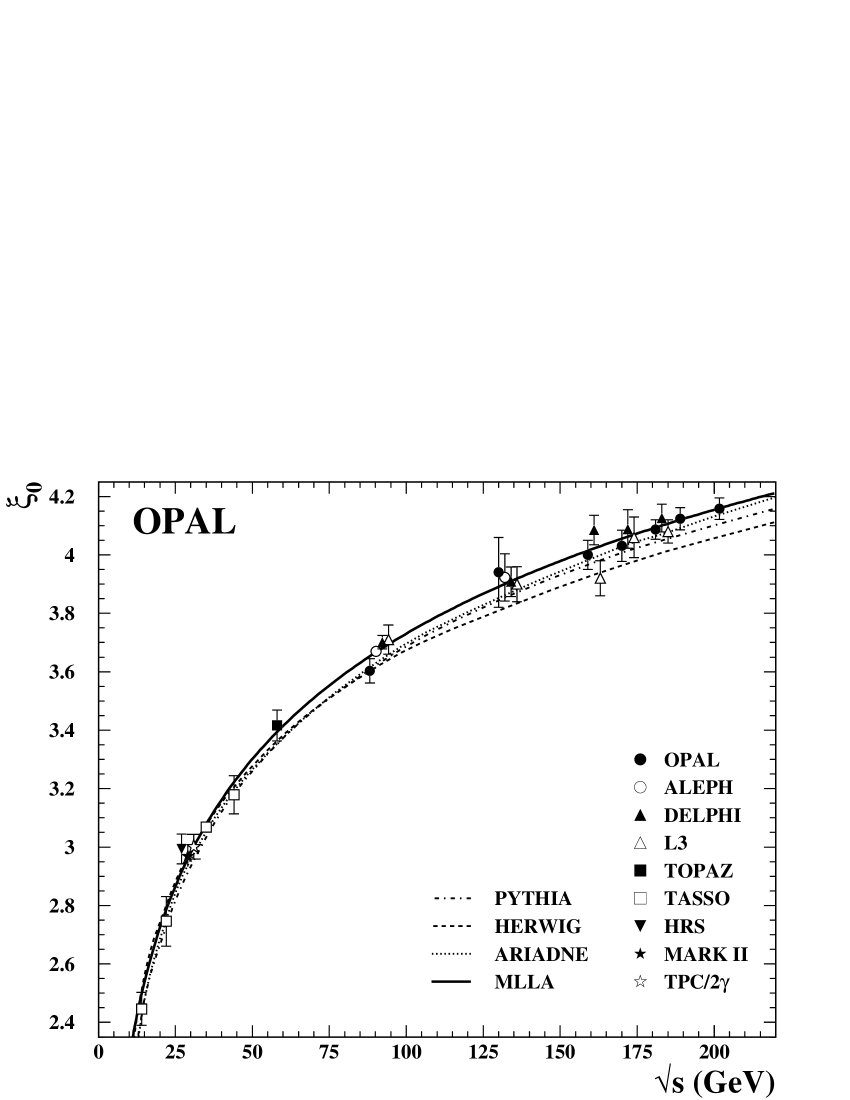
Figure 8: Evolution of the position of the peak in the $\xi_{p}$ distribution, $\xi_{0}$, with c.m. energy, in the range $\sqrt{s}=14-202$ GeV, compared to the fitted MLLA prediction (Equation (8) in this paper) and to predictions of PYTHIA, HERWIG and ARIADNE. The error bars of the data represent the combined statistical and systematic uncertainties.

In Figure 8 our $\xi_{0}$ result is shown together with earlier $\xi_{0}$ results from OPAL [31, 1, 2, 3] and other LEP experiments [5, 37, 38] and the $\xi_{0}$ values we determined for the lower energy experiments [32, 33, 39, 40, 41]. The results are compared to the predictions of PYTHIA, HERWIG and ARIADNE and to the fitted prediction of Equation (8). For the fit three active flavours were assumed and the scale, $\Lambda$, was the only free parameter. The fit yields $\Lambda=203\pm 2$ MeV, where the error is the fit uncertainty. The fitted MLLA prediction is in good agreement with the data. The PYTHIA and ARIADNE predictions are slightly below the data, while the HERWIG prediction, in particular at the highest c.m. energies, is much lower than the data.

5.2 Comparisons to theory at high $x$

Another theoretical framework for momentum distributions is formulated in terms of the scale evolution of fragmentation functions. In this framework, a factorisation between the perturbative scattering process on one hand, and the parton emission cascade and non-perturbative hadronisation stage on the other hand, is formulated as follows (see e.g. [42, 43, 44]):

$${{1\over\sigma}{\mathrm{d}\sigma^{h}\over\mathrm{d}x}} = \int_{x}^{1}{\mathrm{d}z\over z}\sum_{f=g,u,d,s,c,b}C_{f}(z,\alpha_{s},\sqrt{s}\,)D^{h}_{f}({x\over z},\mu).$$ (9)

The $C_{f}(x,\alpha_{s},\sqrt{s})$ are coefficient functions, describing the probability to obtain a parton $f$ (gluon, $g$, or quark, $u,d,s,c,b$) with energy fraction $x$ in an $\mathrm{e^{+}e^{-}}$ collision, and $D^{h}_{f}(x,\mu)$ are fragmentation functions, describing the expected distribution of final state hadrons $h$ from an initial parton $f$ at scale $\mu$. The $x$ dependence of fragmentation functions is not known a priori, but their dependence on the energy scale is predicted by theory. In QCD this scale dependence, also known as scaling violation, is described by parton evolution equations [45], or “DGLAP” equations. These equations, as well as the coefficient functions of Equation (9), are currently known to next-to-leading order (NLO) accuracy in $\alpha_{s}$ [46, 42, 43, 44].

Using a computer program [47] written for scaling violation analyses of proton structure functions in NLO QCD, to which we added NLO evolution equations for fragmentation functions and NLO coefficient functions for $\mathrm{e^{+}e^{-}}$ annihilation, we performed a fit of Equation (9) to OPAL and lower energy data. These data include the inclusive charged particle $x_{p}$ distributions measured here and at lower energies [50, 1, 2, 3, 32, 39, 48, 49], flavour tagged $x_{p}$ distributions [50], and results on the helicity components in charged particle production [51].

The fit involves defining fragmentation functions $D^{h}_{f}(x,\mu_{0})$ at an arbitrarily chosen input scale, $\mu_{0}$, evolving these over the entire relevant range of scales using the parton evolution equations, and using them to calculate the theory expectation for the measured distributions (Equation (9)). The a priori unknown input consists of the input fragmentation functions and the strong coupling constant $\alpha_{s}$. The fragmentation functions are parameterised, similarly to reference [51], as

$$xD^{h}_{i}(x,\mu_{0}) = N_{i}(1-x)^{\alpha_{i}}x^{\beta_{i}}e^{-c_{i}(\ln{x})^{2}},$$ (10)

where the parameters $N_{i}$, $\alpha_{i}$, $\beta_{i}$ and $c_{i}$ are determined independently for $i=g,u,(ds),c,b$. The separation between the fragmentation functions of the different quark flavours relies on the $(uds)$, $c$ and $b$ flavour tagged data included in the fit and on the fact that as a consequence of the different electric and weak charges the relative contributions from $d$, $s$ and $b$ quarks compared those from $u$ and $c$ quarks, vary with the c.m. energy. No data included in the fit provide information to separate the contributions from $d$ and $s$ quarks. Therefore only one fragmentation function is defined for these two flavours.

In earlier studies [42, 44, 52, 53, 54], similar fits were performed, including data up to c.m. energies of 91 GeV, to obtain measurements of $\alpha_{s}$. The higher energy LEP 2 data do not add significantly to the achievable precision on $\alpha_{s}$, which is mostly constrained by the very precise low energy and LEP 1 results. We therefore choose, in our default fit, to fix $\alpha_{s}$ at its current best estimate of $\alpha_{s}(M_{\mathrm{Z}})=0.1181\pm 0.002$ [55], to test how well the fitted predictions describe the data over the now extended range of scales. The data included in the fit are restricted to $x_{p}$ values between 0.07 and 0.80. In addition, the particle momenta were required to be greater than 1 GeV/$c$, effectively raising the lower $x_{p}$ limit for the lowest energy experiments. This cut is motivated by the fact that the present formalism does not account for destructive interference effects in soft gluon emissions (see Section 5.1).

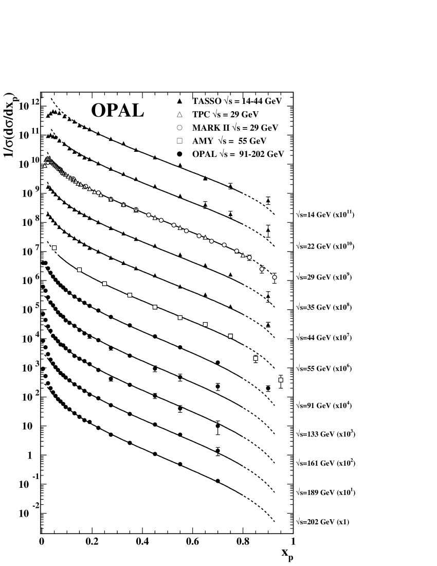
Figure 9: $x_{p}$ spectra measured in the range $\sqrt{s}=14-202$ GeV, compared to fitted NLO predictions (Equation (9) in this paper) using the world average value of $\alpha_{s}(M_{\mathrm{Z}})=0.1181$. The full lines indicate the region of the fit. The uncertainties of the data represent the combined statistical and systematic errors.

In Figure 9, $x_{p}$ distributions measured at c.m. energies from 14 to 202 GeV are compared to the fitted predictions. The theory predictions are in good agreement with the data in the fitted range (full lines). The total $\chi^{2}$ of the fit is 198 for 188 degrees of freedom. As for the fits described in Section 5.1, this $\chi^{2}$ result is based on the full (statistical and systematic) uncertainties on the data and neglects any correlations between data points. Outside the fitted range, at low $x_{p}$ and low c.m. energies, charged particle production is suppressed. This suppression is not described by the predictions, which do not include soft gluon interference effects, as stated above.

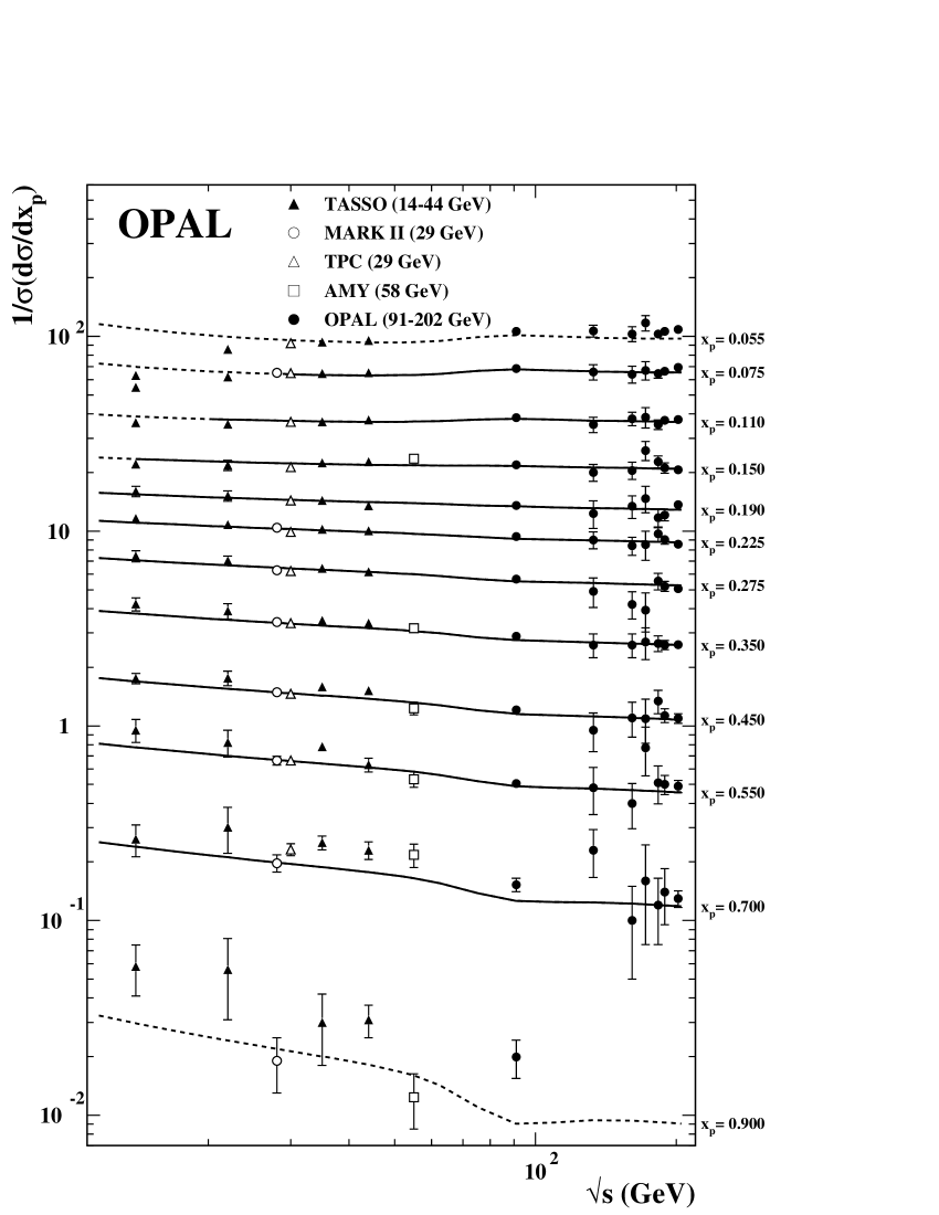
Figure 10: Inclusive charged particle rate, $1/\sigma\cdot\mathrm{d}\sigma_{\mathrm{ch}}/\mathrm{d}x_{p}$, as a function of $\sqrt{s}$ in bins of $x_{p}$, compared to fitted NLO predictions (Equation (9) in this paper) using the world average value of $\alpha_{s}(M_{\mathrm{Z}})=0.1181$. The full lines indicate the region of the fit. The uncertainties of the data represent the combined statistical and systematic errors.

Scaling violations in charged particle production are shown in Figure 10, where the $1/\sigma\cdot\mathrm{d}\sigma_{\mathrm{ch}}/\mathrm{d}x_{p}$ results are shown as a function of $\sqrt{s}$ for a number of $x_{p}$ bins. Negative scaling violations are visible for the higher $x_{p}$ values. At low $x_{p}$ the charged particle production rate demonstrates little dependence on the c.m. energy. Changes in the flavour composition with c.m. energy also influence the observed level of scaling violations, especially at high $x_{p}$ and around $\sqrt{s}=91$ GeV where a relatively large fraction of events is expected to contain $b$ quarks.

The data in Figure 10 are also compared to the fitted NLO predictions. Overall, a good agreement between data and theory is found in the region of the fit (full lines). We thus conclude that inclusive charged particle production data can be described by the QCD based parton evolution formalism, using the world-average value for $\alpha_{s}$. When we leave $\alpha_{s}$ as a free parameter in the fit, we obtain $\alpha_{s}(M_{\mathrm{Z}})=0.113\pm 0.005\pm 0.007$, where the first error is the fit uncertainty and the second the uncertainty obtained by independently varying the renormalisation and factorisation scales up and down by a factor 2. For the dependence of Equation (9) and the parton evolution equations on these scales we refer to [45, 46, 42, 43, 44].

6 Summary and conclusion

We have presented a measurement of charged particle momentum distributions in hadronic $\mathrm{e^{+}e^{-}}$ annihilation events produced at LEP 2 at c.m. energies between 192 and 209 GeV. The results are combined into a single set of distributions, corresponding to an average c.m. energy of $\langle\sqrt{s}\,\rangle=201.7$ GeV.

The results, in combination with those obtained at lower c.m. energies, were compared to QCD Monte Carlo models and to analytical QCD predictions calculated in various approaches. In general, good agreement is observed between the data and these theory predictions in the regions where the latter are expected to be valid.

$\sqrt{s}$ range (GeV)	191 – 193	195 – 197	199 – 201
$\langle\sqrt{s}\,\rangle$ (GeV)	191.6	195.5	199.5
Integrated luminosity ($\mathrm{pb}^{-1}$)	$29.15\pm 0.09$	$72.57\pm 0.19$	$74.51\pm 0.20$
Preselection	2796	6820	6262
Expected	$2769\pm 8$	$6448\pm 16$	$6284\pm 15$
4-fermion background (%)	$20.1\pm 0.1$	$21.9\pm 0.1$	$24.8\pm 0.1$
Eff. non-rad. events (%)	$98.4\pm 0.1$	$98.3\pm 0.1$	$98.5\pm 0.1$
“ISR-fit” Selection	765	1848	1734
Expected	$745\pm 4$	$1793\pm 8$	$1771\pm 8$
4-fermion background (%)	$30.2\pm 0.3$	$31.8\pm 0.3$	$33.6\pm 0.3$
Eff. non-rad. events (%)	$89.9\pm 0.3$	$90.0\pm 0.2$	$89.8\pm 0.2$
Final selection	507	1111	1047
Expected	$461\pm 4$	$1074\pm 6$	$1039\pm 6$
4-fermion background (%)	$4.6\pm 0.1$	$4.6\pm 0.1$	$5.3\pm 0.1$
Eff. non-rad. events (%)	$77.0\pm 0.4$	$76.3\pm 0.3$	$76.1\pm 0.3$
$\sqrt{s}$ range (GeV)	201 – 202.5	202.5 – 205.5	205.5 – 209.5
$\langle\sqrt{s}\,\rangle$ (GeV)	201.6	204.9	206.6
Integrated luminosity ($\mathrm{pb}^{-1}$)	$37.97\pm 0.11$	$81.96\pm 0.19$	$137.14\pm 0.29$
Preselection	2971	6031	9847
Expected	$3021\pm 8$	$6240\pm 16$	$10114\pm 26$
4-fermion background (%)	$24.4\pm 0.1$	$25.8\pm 0.2$	$26.5\pm 0.2$
Eff. non-rad. events (%)	$98.3\pm 0.1$	$98.5\pm 0.1$	$98.4\pm 0.1$
“ISR-fit” Selection	838	1781	2840
Expected	$881\pm 4$	$1857\pm 8$	$3052\pm 14$
4-fermion background (%)	$33.7\pm 0.3$	$34.5\pm 0.3$	$34.8\pm 0.3$
Eff. non-rad. events (%)	$89.4\pm 0.2$	$89.8\pm 0.2$	$89.7\pm 0.2$
Final selection	494	1091	1647
Expected	$514\pm 3$	$1075\pm 6$	$1758\pm 10$
4-fermion background (%)	$5.2\pm 0.1$	$5.6\pm 0.2$	$5.7\pm 0.2$
Eff. non-rad. events (%)	$75.6\pm 0.3$	$75.8\pm 0.3$	$75.9\pm 0.3$

Table 1: Data samples corresponding to six ranges in c.m. energy. The luminosities and the luminosity weighted mean c.m. energies are given in the first two rows. The rows labelled as “Preselection”, “ISR-fit selection” and “Final selection” correspond to the number of events passing these criteria. For each of these selection stages the expected number of events, the remaining fraction of 4-fermion background and the signal efficiency are also given. The errors on the integrated luminosity include statistical and systematic uncertainties added in quadrature. All other errors are the statistical errors only.

$p_{\perp}^{\mathrm{in}}$ (GeV/$c$)	$1/\sigma\cdot\mathrm{d}\sigma_{\mathrm{ch}}/\mathrm{d}$$p_{\perp}^{\mathrm{in}}$ $({\rm GeV}/c)^{-1}$
0.00-0.10	55.8 $\pm$	0.4 $\pm$	2.0
0.10-0.20	44.8 $\pm$	0.3 $\pm$	1.4
0.20-0.30	33.58 $\pm$	0.29 $\pm$	0.80
0.30-0.40	25.35 $\pm$	0.24 $\pm$	0.42
0.40-0.50	18.73 $\pm$	0.21 $\pm$	0.18
0.50-0.60	14.83 $\pm$	0.19 $\pm$	0.10
0.60-0.70	11.49 $\pm$	0.17 $\pm$	0.15
0.70-0.80	9.48 $\pm$	0.15 $\pm$	0.16
0.80-0.90	7.71 $\pm$	0.14 $\pm$	0.16
0.90-1.00	6.46 $\pm$	0.13 $\pm$	0.07
1.00-1.20	4.926 $\pm$	0.083 $\pm$	0.048
1.20-1.40	3.689 $\pm$	0.073 $\pm$	0.038
1.40-1.60	2.933 $\pm$	0.064 $\pm$	0.057
1.60-2.00	2.052 $\pm$	0.043 $\pm$	0.054
2.00-2.50	1.240 $\pm$	0.030 $\pm$	0.045
2.50-3.00	0.754 $\pm$	0.023 $\pm$	0.019
3.00-3.50	0.528 $\pm$	0.020 $\pm$	0.023
3.50-4.00	0.360 $\pm$	0.016 $\pm$	0.020
4.00-5.00	0.217 $\pm$	0.010 $\pm$	0.011
5.00-6.00	0.123 $\pm$	0.008 $\pm$	0.007
6.00-7.00	0.074 $\pm$	0.006 $\pm$	0.005
7.00-8.00	0.054 $\pm$	0.005 $\pm$	0.006

Table 2: Measured values of the distribution $1/\sigma\cdot\mathrm{d}\sigma_{\mathrm{ch}}/\mathrm{d}$$p_{\perp}^{\mathrm{in}}$ at $\langle\sqrt{s}\,\rangle=201.7$ GeV. The first error is statistical, the second systematic.

$p_{\perp}^{\mathrm{out}}$ (GeV/$c$)	$1/\sigma\cdot\mathrm{d}\sigma_{\mathrm{ch}}/\mathrm{d}$$p_{\perp}^{\mathrm{out}}$ $({\rm GeV}/c)^{-1}$
0.00-0.10	81.7 $\pm$	0.5 $\pm$	2.0
0.10-0.20	62.2 $\pm$	0.4 $\pm$	1.2
0.20-0.30	43.39 $\pm$	0.33 $\pm$	0.46
0.30-0.40	28.93 $\pm$	0.27 $\pm$	0.31
0.40-0.50	19.14 $\pm$	0.22 $\pm$	0.25
0.50-0.60	12.60 $\pm$	0.18 $\pm$	0.29
0.60-0.70	8.49 $\pm$	0.15 $\pm$	0.21
0.70-0.80	6.08 $\pm$	0.13 $\pm$	0.17
0.80-0.90	4.14 $\pm$	0.11 $\pm$	0.07
0.90-1.00	3.143 $\pm$	0.098 $\pm$	0.054
1.00-1.20	1.883 $\pm$	0.059 $\pm$	0.072
1.20-1.40	1.266 $\pm$	0.049 $\pm$	0.064
1.40-1.60	0.798 $\pm$	0.040 $\pm$	0.042
1.60-2.00	0.445 $\pm$	0.024 $\pm$	0.017
2.00-2.40	0.237 $\pm$	0.020 $\pm$	0.025
2.40-2.80	0.102 $\pm$	0.014 $\pm$	0.034
2.80-3.20	0.047 $\pm$	0.011 $\pm$	0.018
3.20-3.60	0.035 $\pm$	0.011 $\pm$	0.026

Table 3: Measured values of the distribution $1/\sigma\cdot\mathrm{d}\sigma_{\mathrm{ch}}/\mathrm{d}$$p_{\perp}^{\mathrm{out}}$ at $\langle\sqrt{s}\,\rangle=201.7$ GeV. The first error is statistical, the second systematic.

$y$	$1/\sigma\cdot\mathrm{d}\sigma_{\mathrm{ch}}/\mathrm{d}$$y$
0.00-0.33	7.44 $\pm$	0.12 $\pm$	0.34
0.33-0.67	8.26 $\pm$	0.13 $\pm$	0.34
0.67-1.00	8.22 $\pm$	0.12 $\pm$	0.25
1.00-1.33	8.26 $\pm$	0.11 $\pm$	0.15
1.33-1.67	8.08 $\pm$	0.10 $\pm$	0.12
1.67-2.00	7.65 $\pm$	0.09 $\pm$	0.09
2.00-2.33	7.18 $\pm$	0.08 $\pm$	0.10
2.33-2.67	6.56 $\pm$	0.07 $\pm$	0.12
2.67-3.00	5.91 $\pm$	0.06 $\pm$	0.15
3.00-3.33	5.12 $\pm$	0.06 $\pm$	0.17
3.33-3.67	4.14 $\pm$	0.05 $\pm$	0.14
3.67-4.00	3.034 $\pm$	0.047 $\pm$	0.088
4.00-4.33	1.936 $\pm$	0.039 $\pm$	0.050
4.33-4.67	1.118 $\pm$	0.029 $\pm$	0.022
4.67-5.00	0.588 $\pm$	0.021 $\pm$	0.014
5.00-5.33	0.258 $\pm$	0.013 $\pm$	0.014
5.33-5.67	0.108 $\pm$	0.009 $\pm$	0.008
5.67-6.00	0.049 $\pm$	0.006 $\pm$	0.003
6.00-6.33	0.011 $\pm$	0.003 $\pm$	0.001

Table 4: Measured values of the distribution $1/\sigma\cdot\mathrm{d}\sigma_{\mathrm{ch}}/\mathrm{d}$$y$ at $\langle\sqrt{s}\,\rangle=201.7$ GeV. The first error is statistical, the second systematic.

$x_{p}$	$1/\sigma\cdot\mathrm{d}\sigma_{\mathrm{ch}}/\mathrm{d}$$x_{p}$
0.00-0.01	927. $\pm$	7. $\pm$	23.
0.01-0.02	522. $\pm$	4. $\pm$	10.
0.02-0.03	296.4 $\pm$	2.8 $\pm$	6.0
0.03-0.04	199.8 $\pm$	2.2 $\pm$	3.9
0.04-0.05	144.2 $\pm$	1.9 $\pm$	3.3
0.05-0.06	108.4 $\pm$	1.6 $\pm$	2.3
0.06-0.07	84.0 $\pm$	1.3 $\pm$	2.2
0.07-0.08	69.4 $\pm$	1.2 $\pm$	1.5
0.08-0.09	57.6 $\pm$	1.1 $\pm$	1.4
0.09-0.10	45.2 $\pm$	1.0 $\pm$	1.0
0.10-0.12	37.4 $\pm$	0.6 $\pm$	1.1
0.12-0.14	27.59 $\pm$	0.55 $\pm$	0.72
0.14-0.16	20.60 $\pm$	0.47 $\pm$	0.69
0.16-0.18	15.76 $\pm$	0.42 $\pm$	0.35
0.18-0.20	13.69 $\pm$	0.39 $\pm$	0.34
0.20-0.25	8.57 $\pm$	0.19 $\pm$	0.17
0.25-0.30	5.06 $\pm$	0.15 $\pm$	0.17
0.30-0.40	2.61 $\pm$	0.07 $\pm$	0.11
0.40-0.50	1.092 $\pm$	0.045 $\pm$	0.041
0.50-0.60	0.489 $\pm$	0.029 $\pm$	0.019
0.60-0.80	0.130 $\pm$	0.009 $\pm$	0.008

Table 5: Measured values of the distribution $1/\sigma\cdot\mathrm{d}\sigma_{\mathrm{ch}}/\mathrm{d}$$x_{p}$ at $\langle\sqrt{s}\,\rangle=201.7$ GeV. The first error is statistical, the second systematic.

$\xi_{p}$	$1/\sigma\cdot\mathrm{d}\sigma_{\mathrm{ch}}/\mathrm{d}$$\xi_{p}$
0.00-0.20	0.015 $\pm$	0.003 $\pm$	0.006
0.20-0.40	0.063 $\pm$	0.006 $\pm$	0.016
0.40-0.60	0.157 $\pm$	0.011 $\pm$	0.014
0.60-0.80	0.370 $\pm$	0.018 $\pm$	0.018
0.80-1.00	0.588 $\pm$	0.024 $\pm$	0.029
1.00-1.20	1.012 $\pm$	0.033 $\pm$	0.043
1.20-1.40	1.398 $\pm$	0.039 $\pm$	0.047
1.40-1.60	1.936 $\pm$	0.045 $\pm$	0.044
1.60-1.80	2.575 $\pm$	0.053 $\pm$	0.060
1.80-2.00	3.106 $\pm$	0.058 $\pm$	0.075
2.00-2.20	3.82 $\pm$	0.06 $\pm$	0.11
2.20-2.40	4.19 $\pm$	0.07 $\pm$	0.11
2.40-2.60	5.02 $\pm$	0.07 $\pm$	0.12
2.60-2.80	5.39 $\pm$	0.08 $\pm$	0.12
2.80-3.00	5.93 $\pm$	0.08 $\pm$	0.13
3.00-3.20	6.42 $\pm$	0.09 $\pm$	0.14
3.20-3.40	6.85 $\pm$	0.09 $\pm$	0.15
3.40-3.60	7.02 $\pm$	0.09 $\pm$	0.15
3.60-3.80	7.33 $\pm$	0.09 $\pm$	0.13
3.80-4.00	7.63 $\pm$	0.10 $\pm$	0.15
4.00-4.20	7.50 $\pm$	0.10 $\pm$	0.14
4.20-4.40	7.63 $\pm$	0.10 $\pm$	0.13
4.40-4.60	7.37 $\pm$	0.10 $\pm$	0.09
4.60-4.80	7.39 $\pm$	0.10 $\pm$	0.09
4.80-5.00	6.75 $\pm$	0.09 $\pm$	0.15
5.00-5.20	6.18 $\pm$	0.09 $\pm$	0.18
5.20-5.40	5.55 $\pm$	0.08 $\pm$	0.20
5.40-5.60	4.97 $\pm$	0.08 $\pm$	0.17
5.60-5.80	4.03 $\pm$	0.07 $\pm$	0.17
5.80-6.00	3.34 $\pm$	0.06 $\pm$	0.18
6.00-6.20	2.50 $\pm$	0.06 $\pm$	0.17

Table 6: Measured values of the distribution $1/\sigma\cdot\mathrm{d}\sigma_{\mathrm{ch}}/\mathrm{d}$$\xi_{p}$ at $\langle\sqrt{s}\,\rangle=201.7$ GeV. The first error is statistical, the second systematic.

Figure 1: Integrated luminosity collected by OPAL in 1999 and 2000 at different c.m. energies.

Figure 4: Distributions of the charged particle momenta (a) $p_{\perp}^{\mathrm{in}}$ and (b) $p_{\perp}^{\mathrm{out}}$ and of the rapidity (c) $y$ at $\langle\sqrt{s}\,\rangle=201.7$ GeV, compared to the corresponding PYTHIA, HERWIG and ARIADNE predictions. The statistical errors and the combined statistical and systematic errors are shown as the inner and outer error bars, respectively.

Figure 5: Distributions of the charged particle fractional momenta (a) $x_{p}$ and (b) $\xi_{p}$ at $\langle\sqrt{s}\,\rangle=201.7$ GeV, compared to the corresponding PYTHIA, HERWIG and ARIADNE predictions. The statistical errors and the combined statistical and systematic errors are shown as the inner and outer error bars, respectively.

Figure 6: $\xi_{p}$ spectra measured in the range $\sqrt{s}=14-202$ GeV, compared to the Fong and Webber [30] predictions (Equation (2) in this paper), fitted to the data. The full lines indicate the region of the fit. For clarity, not all OPAL data included in the fit are shown in the figure. The error bars on the data represent the combined statistical and systematic uncertainties.

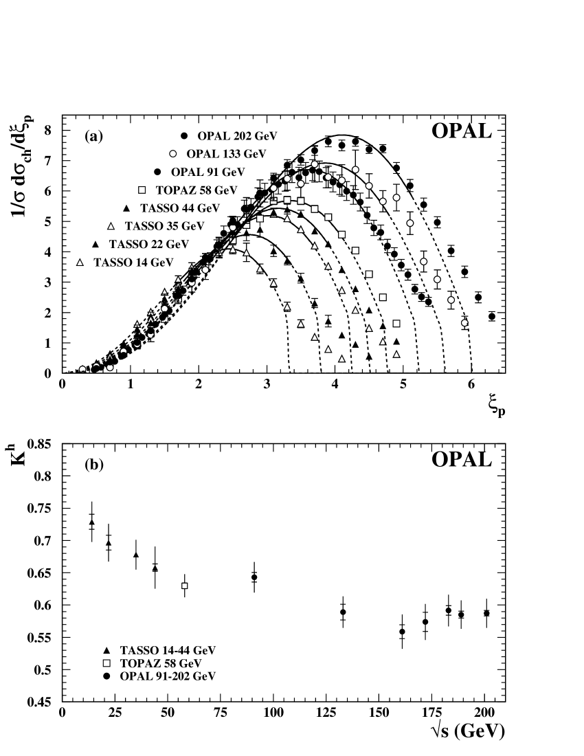
Figure 7: a) $\xi_{p}$ spectra measured in the range $\sqrt{s}=14-202$ GeV, compared to MLLA predictions in the limiting spectrum approach ([28], Equation (7) in this paper), fitted to the data. The full lines indicate the region of the fit. For clarity, not all OPAL data included in the fit are shown in the figure. The error bars on the data represent the combined statistical and systematic uncertainties.
b) The hadronisation constants $K^{h}$ at different $\sqrt{s}$ as obtained from the fit, described in Section 5.1.2. The inner error bar represents the fit error and the outer error bar the combined fit error and the error obtained from varying the fit range.

References

- [1] OPAL Collaboration, G. Alexander et al., Z. Phys. C72 (1996) 191
- [2] OPAL Collaboration, K. Ackerstaff et al., Z. Phys. C75 (1997) 193
- [3] OPAL Collaboration, G. Abbiendi et al., Eur. Phys. J. C16 (2000) 185
- [4] ALEPH Collaboration, D. Busculic et al., Z. Phys. C73 (1997) 409
- [5] L3 Collaboration, M. Acciarri et al., Phys. Lett. B444 (1998) 569
- [6] DELPHI Collaboration, P. Abreu et al., Z. Phys. C73 (1997) 229
- [7] OPAL Collaboration, K. Ahmet et al., Nucl. Instrum. Methods A305 (1991) 275
- [8] J. Allison et al., Nucl. Instrum. Methods A317 (1992) 47
- [9] T. Sjöstrand, Comput. Phys. Commun. 82 (1994) 74
- [10] T. Sjöstrand et al., Comput. Phys. Commun. 135 (2001) 238
- [11] S. Jadach, B.F.L. Ward and Z. Wa̧s, Comput. Phys. Commun. 130 (2000) 260
- [12] OPAL Collaboration, G. Alexander et al., Z. Phys. C69 (1996) 543
- [13] G. Marchesini et al., Comput. Phys. Commun. 67 (1992) 465
- [14] J. Fujimoto et al., Comput. Phys. Commun. 100 (1997) 128
-
[15]
J.A.M. Vermaseren, J. Smith and G. Grammer Jr., Phys. Rev. D19 (1979) 137;
J.A.M. Vermaseren, Nucl. Phys. B229 (1983) 347 -
[16]
R. Engel, Z. Phys. C66 (1995) 203;
R. Engel and J. Ranft, Phys. Rev. D54 (1996) 4244 - [17] S. Jadach et al., Comput. Phys. Commun. 76 (1993) 361
- [18] L. Lönnblad, Comput. Phys. Commun. 71 (1992) 15 v4
-
[19]
ALEPH Collaboration, R. Barate et al., Phys. Rept. 294 (1998) 1;
OPAL Collaboration, G. Abbiendi et al., Eur. Phys. J. C11 (1999) 217 - [20] OPAL Collaboration, G. Alexander et al., Z. Phys. C52 (1991) 175
- [21] OPAL Collaboration, K. Ackerstaff et al., Phys. Lett. B391 (1997) 221
- [22] S. Catani et al., Phys. Lett. B269 (1991) 432
- [23] OPAL Collaboration, K. Ackerstaff et al., Eur. Phys. J. C2 (1998) 213
- [24] S. Catani and M.H. Seymour, Phys. Lett. B378 (1996) 287
- [25] R.K. Ellis, D.A. Ross and A.E. Terrano, Nucl. Phys. B178 (1981) 421
- [26] OPAL Collaboration, G. Abbiendi et al., Phys. Lett. B493 (2000) 249
-
[27]
Ya.I. Azimov et al., Z. Phys. C27 (1985) 65;
Ya.I. Azimov et al., Z. Phys. C31 (1986) 213 - [28] V.A. Khoze and W. Ochs, Int. J. of Mod. Phys. A12 (1997) 2949
- [29] Yu.L. Dokshitzer, V.S. Fadin and V.A. Khoze, Phys. Lett. B115 (1982) 242
- [30] C.P. Fong and B.R. Webber, Nucl. Phys. B355 (1991) 54
- [31] OPAL Collaboration, M.Z. Akrawy et al., Phys. Lett. B247 (1990) 617
- [32] TASSO Collaboration, W. Braunschweig et al., Z. Phys. C47 (1990) 187
- [33] TOPAZ Collaboration, R. Itoh et al., Phys. Lett. B345 (1995) 335
- [34] Yu.L. Dokshitzer, V.S. Fadin and V.A. Khoze, Z. Phys. C15 (1982) 325
- [35] Yu.L. Dokshitzer, V.A. Khoze and S.I. Troyan, J. Phys. G17 (1991) 1481
- [36] Yu.L. Dokshitzer, V.A. Khoze and S.I. Troyan, Int. J. Mod. Phys. A7 (1992) 1875
- [37] ALEPH Collaboration, R. Barate et al., Phys. Rept. 294 (1998) 1
- [38] DELPHI Collaboration, P. Abreu et al., Phys. Lett. B459 (1999) 397
-
[39]
TPC/2 Collaboration, H. Aihara et al., Phys. Rev. Lett. 61 (1988) 1263;
G.D. Cowan, Ph.D. Thesis (LBL, Berkeley) LBL-24715 (1988) - [40] MARK II Collaboration, J.F. Patrick et al., Phys. Rev. Lett. 49 (1982) 1232
- [41] HRS Collaboration, D. Bender et al., Phys. Rev. D31 (1985) 1
- [42] P. Nason and B.R. Webber, Nucl. Phys. B421 (1994) 473
-
[43]
P.J. Rijken and W.L. van Neerven, Phys. Lett. B386 (1996) 422;
P.J. Rijken and W.L. van Neerven, Nucl. Phys. B487 (1997) 233 - [44] J. Binnewies, Ph.D. Thesis (Hamburg U.) DESY 97-128 (1997)
-
[45]
V.N. Gribov and L.N. Lipatov, Sov. J. Nucl. Phys. 15 (1972) 438;
G. Altarelli and G. Parisi, Nucl. Phys. B126 (1977) 298;
Yu.L. Dokshitzer, Sov. Phys. JETP 46 (1977) -
[46]
W. Furmanski and R. Petronzio, Phys. Lett. B97 (1980) 437;
G. Curci, W. Furmanski and R. Petronzio, Nucl. Phys. B175 (1980) 27;
W. Furmanski and R. Petronzio, Z. Phys. C11 (1982) 293 -
[47]
M. Botje, “QCDNUM version 16.12”, ZEUS-97-066 (unpublished), see
http,//www.nikhef.nl/user/h24/qcdnum - [48] AMY Collaboration, Y.K. Li et al., Phys. Rev. D41 (1990) 2675
- [49] MARK II Collaboration, A. Petersen et al., Phys. Rev. D37 (1988) 1
- [50] OPAL Collaboration, K. Ackerstaff et al., Eur. Phys. J. C7 (1999) 369
- [51] OPAL Collaboration, R. Akers et al., Z. Phys. C68 (1995) 203
- [52] ALEPH Collaboration, D. Buskulic et al., Phys. Lett. B357 (1995) 487
- [53] DELPHI Collaboration, P. Abreu, Phys. Lett. B398 (1997) 194
- [54] B.A. Kniehl, G. Kramer and B. Pötter, Nucl. Phys. B582 (2000) 514
- [55] D.E. Groom et al., Eur. Phys. J. C15 (2000) 1