A Measurement of the $\tau^{-}\rightarrow\mu^{-}\bar{\nu}_{\mu}\nu_{\tau}$ Branching Ratio

Abstract

The $\tau^{-}\rightarrow\mu^{-}\bar{\nu}_{\mu}\nu_{\tau}$ branching ratio has been measured using data collected from 1990 to 1995 by the OPAL detector at the LEP collider. The resulting value of $\mbox{B($\tau^{-}\rightarrow\mu^{-}\bar{\nu}_{\mu}\nu_{\tau}$)}=0.1734\pm 0.0009(stat)\pm 0.0005(syst)$ has been used in conjunction with other OPAL measurements to test lepton universality, yielding the coupling constant ratios $g_{\mu}/g_{\mathrm{e}}=1.0005\pm 0.0043$ and $g_{\tau}/g_{\mathrm{e}}=1.0031\pm 0.0047$, in good agreement with the Standard Model prediction of unity, and also to determine a value for the Michel parameter $\eta=0.004\pm 0.036$. This is subsequently used to find a model-dependent limit of the mass for the charged Higgs boson, $m_{\mathrm{H}^{\pm}}>1.30\tan\beta$, in the Minimal Supersymmetric Standard Model framework.

1 Introduction

Precise measurements of the leptonic decays of $\tau$ leptons provide a means of stringently testing various aspects of the Standard Model. OPAL previously has studied the leptonic $\tau$ decay modes by measuring the branching ratios [1, 2], the Michel parameters [3], and radiative decays [4]. This work presents a new OPAL measurement of the $\tau^{-}\rightarrow\mu^{-}\bar{\nu}_{\mu}\nu_{\tau}$ branching ratio, using data taken from 1990 to 1995 at energies near the Z⁰ peak, corresponding to an integrated luminosity of approximately 170 pb^-1. A pure sample of $\tau^{+}\tau^{-}$ pairs is selected from the LEP1 data set as described in Section 2, and then the fraction of $\tau$ jets in which the $\tau$ has decayed to a muon is determined, using the selection described in Section 3. This fraction is then corrected for backgrounds, efficiency, and bias, as described in Section 5. The selection of $\tau^{-}\rightarrow\mu^{-}\bar{\nu}_{\mu}\nu_{\tau}$ candidates relies on only a few variables, each of which provides a highly effective means of separating background events from signal events while minimising systematic uncertainty. This new measurement supersedes the previous OPAL measurement of B$(\tau^{-}\rightarrow\mu^{-}\bar{\nu}_{\mu}\nu_{\tau})=0.1736\pm 0.0027$ which was obtained using data collected in 1991 and 1992, corresponding to an integrated luminosity of approximately 39 pb^-1 [2].

OPAL [5] is a general purpose detector covering almost the full solid angle with approximate cylindrical symmetry about the $\mbox{e}^{+}\mbox{e}^{-}$ beam axis. In the OPAL coordinate system, the $e^{-}$ beam direction defines the $+z$ axis, and the $+x$ axis points from the detector towards the centre of the LEP ring. The polar angle $\theta$ is measured from the $+z$ axis, and the azimuthal angle $\phi$ is measured from the $+x$ axis.

Selection efficiencies and kinematic variable distributions were modelled using Monte Carlo simulated $\tau^{+}\tau^{-}$ event samples generated with the KORALZ 4.02 package [6] and the TAUOLA 2.0 library [7]. These events were then passed through a full simulation of the OPAL detector [8]. Background contributions from non-$\tau$ sources were evaluated using Monte Carlo samples based on the following generators: multihadronic events $(\mbox{e}^{+}\mbox{e}^{-}\rightarrow\mbox{q}\overline{\mbox{q}})$ were simulated using JETSET 7.3 and JETSET 7.4 [9], $\mbox{e}^{+}\mbox{e}^{-}\rightarrow\mu^{+}\mu^{-}$ events using KORALZ [6], Bhabha events using BHWIDE [10], and two-photon events using VERMASEREN [11].

2 The $\tau^{+}\tau^{-}$ selection

At LEP1, electrons and positrons were made to collide at centre-of-mass energies close to the Z⁰ peak, producing Z⁰ bosons at rest which subsequently decayed into back-to-back pairs of leptons or quarks, from which the $\tau^{+}\tau^{-}$ pairs were selected for this analysis. These highly relativistic $\tau$ particles decay in flight close to the interaction point, resulting in two highly-collimated, back-to-back jets in the tracking chamber.

The $\tau^{+}\tau^{-}$ selection requires that an event have two jets as defined by the cone algorithm in reference [12], each with a cone half-angle of $35^{\circ}$.

The main sources of background to the $\tau^{+}\tau^{-}$ selection are Bhabha events, dimuon events, multihadron events, and two-photon events. This analysis uses the standard OPAL $\tau^{+}\tau^{-}$ selection [13], which was developed to identify $\tau^{+}\tau^{-}$ pairs and to remove these backgrounds, with slight modifications to further reduce Bhabha background in the $\tau^{+}\tau^{-}$ sample.

For each type of background remaining in the $\tau^{+}\tau^{-}$ sample, a variable was chosen in which the signal and background can be visibly distinguished. The relative proportion of background was enhanced by loosening criteria which would normally remove that particular type of background from the $\tau^{+}\tau^{-}$ sample, and/or by applying further criteria to reduce the contribution from signal and to remove other types of background. A comparison of the data and Monte Carlo distributions was then used to assess the modelling of the background. In most cases, the Monte Carlo simulation was found to be consistent with the data. When the data and Monte Carlo distributions did not agree, the Monte Carlo simulation was adjusted to fit the data. Uncertainties of 4% to 20% were assigned to the background estimates as a result of these comparisons.

The $\tau^{+}\tau^{-}$ selection leaves a sample of 96,898 candidate $\tau^{+}\tau^{-}$ events, with a predicted fractional background of $(0.01055\pm 0.00052)$. The backgrounds in the $\tau^{+}\tau^{-}$ sample are summarised in Table 1. The errors shown in the table include both the statistical and systematic uncertainties. The effect of a small bias in this event selection is discussed in Section 5.1.

Table 1: Fractional backgrounds in the $\tau^{+}\tau^{-}$ sample.

Background	Contamination
$\mbox{e}^{+}\mbox{e}^{-}\rightarrow\mbox{e}^{+}\mbox{e}^{-}$	$0.00305\pm 0.00027$
$\mbox{e}^{+}\mbox{e}^{-}\rightarrow\mu^{+}\mu^{-}$	$0.00108\pm 0.00022$
$\mbox{e}^{+}\mbox{e}^{-}\rightarrow\mbox{q}\overline{\mbox{q}}$	$0.00377\pm 0.00015$
$\mbox{e}^{+}\mbox{e}^{-}\rightarrow(\mbox{e}^{+}\mbox{e}^{-})\;\mu^{+}\mu^{-}$	$0.00108\pm 0.00022$
$\mbox{e}^{+}\mbox{e}^{-}\rightarrow(\mbox{e}^{+}\mbox{e}^{-})\;\mbox{e}^{+}\mbox{e}^{-}$	$0.00157\pm 0.00028$
Total	$0.01055\pm 0.00052$

3 The $\tau^{-}\rightarrow\mu^{-}\bar{\nu}_{\mu}\nu_{\tau}$ selection

After the $\tau^{+}\tau^{-}$ selection, each of the 193,796 candidate $\tau$ jets is analysed individually to see whether it exhibits the characteristics of the required $\tau^{-}\rightarrow\mu^{-}\bar{\nu}_{\mu}\nu_{\tau}$ signature. A muon from a $\tau$ decay will result in a track in the central tracking chamber, little energy in the electromagnetic and hadronic calorimeters, and a track in the muon chambers. The $\tau^{-}\rightarrow\mu^{-}\bar{\nu}_{\mu}\nu_{\tau}$ selection is based primarily on information from the central tracking chamber and the muon chambers. Calorimeter information is not used in the main selection, but instead is used to create an independent $\tau^{-}\rightarrow\mu^{-}\bar{\nu}_{\mu}\nu_{\tau}$ control sample that is used to evaluate the systematic error in the Monte Carlo efficiency prediction. The selection criteria which are used to identify the $\tau^{-}\rightarrow\mu^{-}\bar{\nu}_{\mu}\nu_{\tau}$ candidates are described below.

The $\tau^{-}\rightarrow\mu^{-}\bar{\nu}_{\mu}\nu_{\tau}$ candidates are selected from jets with one to three tracks in the tracking chamber, where the tracks are ordered according to decreasing particle momentum. The highest momentum track is assumed to be the muon candidate.

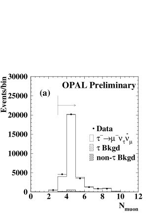
Muons are identified as producing a signal in at least three muon chamber layers, i.e. $N_{\mathrm{muon}}>2$, where $N_{\mathrm{muon}}$ is the number of muon chamber layers activated by a passing particle, as shown in Figure 1 (a) and (b). The value of the $N_{\mathrm{muon}}$ cut was chosen to minimise the background while retaining signal.

Figure 1: ((a) and (b)) The number of muon layers, $N_{\mathrm{muon}}$, activated by the passage of a charged particle in the jet , and ((c) and (d)) the $\mu_{\mathrm{match}}$ matching between a muon track reconstructed in the jet chamber and one reconstructed in the muon chamber. The jets in each plot have passed all other selection criteria. The arrows indicate the accepted regions. The points are data, the clear histogram is the Monte Carlo $\tau^{-}\rightarrow\mu^{-}\bar{\nu}_{\mu}\nu_{\tau}$ prediction, the singly-hatched histogram is the Monte Carlo prediction for backgrounds from other $\tau$ decays, and the cross-hatched histogram is the Monte Carlo prediction for background from non-$\tau$ sources.

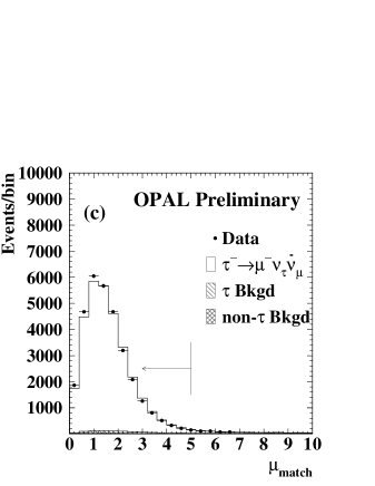
Tracks in the muon chambers are reconstructed independently from those in the tracking chamber. The candidate muon track in the tracking chamber is typically well-aligned with the corresponding track in the muon chambers, whereas this is not the case for hadronic $\tau$ decays, which are the main source of background in the sample. The majority of these background jets contain a pion which interacts in the hadronic calorimeter, resulting in the production of secondary particles which emerge from the calorimeter and generate signals in the muon chambers, a process known as pion punchthrough. Therefore, a “muon matching” variable, $\mu_{\mathrm{match}}$, which compares the agreement between the direction of a track reconstructed in the tracking chamber and that of the track reconstructed in the muon chambers, is used to differentiate the signal $\tau^{-}\rightarrow\mu^{-}\bar{\nu}_{\mu}\nu_{\tau}$ decays from hadronic $\tau$ decays. It is required that $\mu_{\mathrm{match}}$ have a value of less than 5, (see Figure 1 (c) and (d)). The position of the cut was chosen to minimise the background while retaining signal.

In order to reduce background from dimuon events, it is required that the momentum of the highest momentum particle in at least one of the two jets in the event, i.e. $p_{\mathrm{1}}$ in the candidate jet and $p_{\mathrm{1-opp}}$ in the opposite jet, must be less than 40 GeV/c. (See Figure 2 (a).)

Figure 2: (a) The momentum of the highest momentum particle in the opposite jet, $p_{\mathrm{1-opp}}$, where the candidate muon has a momentum greater than 40 GeV/c, and (b) the combined momentum of the second and third particles in the jet, for jets which have passed all other selection criteria. The arrows indicate the accepted regions.

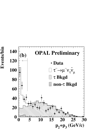
Although the $\tau^{-}\rightarrow\mu^{-}\bar{\nu}_{\mu}\nu_{\tau}$ candidates in general are expected to have one track, in approximately 2% of these decays a radiated photon converts to an $\mbox{e}^{+}\mbox{e}^{-}$ pair, resulting in one or two extra tracks in the tracking chamber. In order to retain these jets but eliminate background jets, it is required that the scalar sum of the momenta of the two lower-momentum particles, $p_{\mathrm{2}}$ + $p_{\mathrm{3}}$, must be less than 4 GeV/c. (See Figure 2 (b).) In cases where there is only one extra track, $p_{\mathrm{3}}$ is taken to be zero.

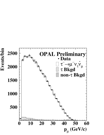
The above criteria leave a sample of 31,395 candidate $\tau^{-}\rightarrow\mu^{-}\bar{\nu}_{\mu}\nu_{\tau}$ jets. The backgrounds remaining in this sample are discussed in the next section. The quality of the data is illustrated in Figure 3, which shows the momentum of the candidate muon for jets which satisfy the $\tau^{-}\rightarrow\mu^{-}\bar{\nu}_{\mu}\nu_{\tau}$ selection criteria.

Figure 3: The momentum of the candidate muon, for jets which have passed all of the selection criteria.

4 Backgrounds in the $\tau^{-}\rightarrow\mu^{-}\bar{\nu}_{\mu}\nu_{\tau}$ sample

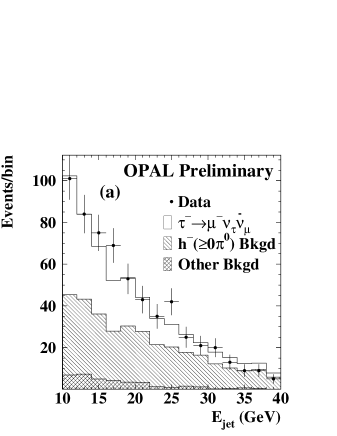
The background contamination in the signal $\tau^{-}\rightarrow\mu^{-}\bar{\nu}_{\mu}\nu_{\tau}$ sample stems from other $\tau$ decay modes and from residual non-$\tau$ background in the $\tau^{+}\tau^{-}$ sample. The procedure used to evaluate the background in the $\tau^{-}\rightarrow\mu^{-}\bar{\nu}_{\mu}\nu_{\tau}$ sample is identical to the one used to evaluate the background in the $\tau^{+}\tau^{-}$ sample, which is outlined in Section 2, and again involves studying the distributions of sensitive variables in background-enhanced samples. It is worth noting that, in all the plots in Figure 4, the relative proportion of background has been enhanced (as in Section 2) in order that the background may be evaluated. The error on each background includes the Monte Carlo statistical error on the background fraction as well as a systematic error associated with the background evaluation.

The main backgrounds from other $\tau$ decay modes can be separated into $\tau^{-}\rightarrow{\mbox{\rm h}}^{-}\geq 0\pi^{0}\nu_{\tau}$, and a small number of $\tau^{-}\rightarrow\mathrm{h}^{-}\mathrm{h}^{-}\mathrm{h}^{+}\geq 0\pi^{0}\nu_{\tau}$ jets. The $\tau^{-}\rightarrow{\mbox{\rm h}}^{-}\geq 0\pi^{0}\nu_{\tau}$ decays can pass the $\tau^{-}\rightarrow\mu^{-}\bar{\nu}_{\mu}\nu_{\tau}$ selection when the charged hadron punches through the calorimeters, leaving a signal in the muon chambers. The absence or presence of $\pi^{0}$s has no impact on whether or not the jet is selected, since there are over 60 radiation lengths of material in the detector in front of the muon chambers. The modelling of this background is tested by studying $\tau^{-}\rightarrow\mu^{-}\bar{\nu}_{\mu}\nu_{\tau}$ jets with large deposits of energy in the electromagnetic calorimeter. The distribution of jet energy, $E_{\mathrm{jet}}$, deposited in the electromagnetic calorimeter is shown in Figure 4 (a). The $\tau^{-}\rightarrow{\mbox{\rm h}}^{-}\geq 0\pi^{0}\nu_{\tau}$ fractional background estimate is $0.0225\pm 0.0016$, of which approximately 75% includes at least one $\pi^{0}$.

Figure 4: The distributions used to measure the background in the $\tau^{-}\rightarrow\mu^{-}\bar{\nu}_{\mu}\nu_{\tau}$ sample are shown. (a) $E_{\mathrm{jet}}$ is the energy measured in the electromagnetic calorimeter, (b) $\theta_{\mathrm{acol}}$ is the acollinearity angle between the two $\tau$ jets, (c) $p_{\mathrm{1-opp}}$ is the momentum of the highest momentum particle in the opposite jet to the $\tau^{-}\rightarrow\mu^{-}\bar{\nu}_{\mu}\nu_{\tau}$ candidate, (d) $\mathrm{d}E/\mathrm{d}x$ is the rate of energy loss of a particle traversing the tracking chamber. The points are data, the clear histogram is the Monte Carlo $\tau^{-}\rightarrow\mu^{-}\bar{\nu}_{\mu}\nu_{\tau}$ prediction, the singly-hatched histogram is the Monte Carlo prediction for the type of background being evaluated using each distribution, and the cross-hatched histogram is the Monte Carlo prediction for all other types of background.

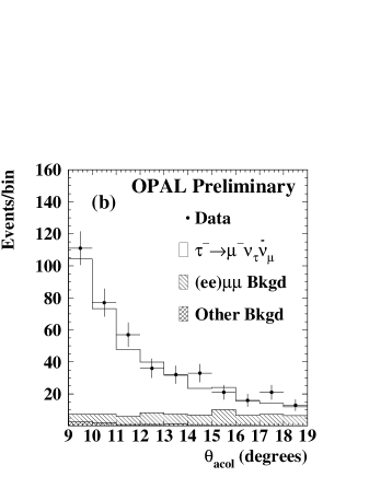
The main backgrounds resulting from contamination in the $\tau^{+}\tau^{-}$ sample are $\mbox{e}^{+}\mbox{e}^{-}\rightarrow(\mbox{e}^{+}\mbox{e}^{-})\;\mu^{+}\mu^{-}$ and $\mbox{e}^{+}\mbox{e}^{-}\rightarrow\mu^{+}\mu^{-}$ events. The $\mbox{e}^{+}\mbox{e}^{-}\rightarrow(\mbox{e}^{+}\mbox{e}^{-})\;\mu^{+}\mu^{-}$ contribution in the $\tau^{-}\rightarrow\mu^{-}\bar{\nu}_{\mu}\nu_{\tau}$ sample was evaluated by fitting the Monte Carlo distribution of the acollinearity angle, $\theta_{\mathrm{acol}}$, to that of the data, as shown in Figure 4 (b). This resulted in a fractional background estimate of $0.0052\pm 0.0010$.

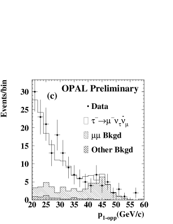
The dimuon jets ($\mbox{e}^{+}\mbox{e}^{-}\rightarrow\mu^{+}\mu^{-}$) were enhanced in the $\tau^{-}\rightarrow\mu^{-}\bar{\nu}_{\mu}\nu_{\tau}$ sample by removing the requirement that $p_{\mathrm{1-opp}}<40$ GeV/c or $p_{\mathrm{1}}<40$ GeV/c, and then requiring that $p_{\mathrm{1}}>40$ GeV/c. The distribution of $p_{\mathrm{1-opp}}$ was then used to evaluate the agreement between the data and the Monte Carlo simulation for this background. The resulting estimate of the dimuon fractional background in the $\tau^{-}\rightarrow\mu^{-}\bar{\nu}_{\mu}\nu_{\tau}$ sample is $0.0029\pm 0.0006$. The corresponding distribution is shown in Figure 4 (c).

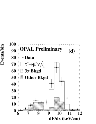
The 3-track signal $\tau^{-}\rightarrow\mu^{-}\bar{\nu}_{\mu}\nu_{\tau}$ is due to photons which convert in the tracking chamber to an $\mbox{e}^{+}\mbox{e}^{-}$ pair, whereas the 3-track background consists mainly of jets with three pions in the final state. Electrons and pions have different rates of energy loss in the OPAL tracking chamber, and hence the background can be isolated from the signal by plotting the rate of energy loss as the particle traverses the tracking chamber, $\mathrm{d}E/\mathrm{d}x$, of the second-highest-momentum particle in the jet. The Monte Carlo modelling was compared to the data as shown in Figure 4 (d), yielding a fractional background measurement of $0.0014\pm 0.0003$.

The remaining background in the $\tau^{-}\rightarrow\mu^{-}\bar{\nu}_{\mu}\nu_{\tau}$ sample consists almost entirely of $\tau^{-}\rightarrow\pi^{-}\pi^{0}\eta\nu_{\tau}$ jets, and contributes at a level of 0.04% to the overall sample. The total estimated fractional background in the $\tau^{-}\rightarrow\mu^{-}\bar{\nu}_{\mu}\nu_{\tau}$ sample after the selection is $0.0324\pm 0.0020$. The main background contributions are summarised in Table 2. The errors in the table include both the statistical and systematic uncertainties.

Table 2: The main sources of background in the candidate $\tau^{-}\rightarrow\mu^{-}\bar{\nu}_{\mu}\nu_{\tau}$ sample.

Backgrounds	Contamination
$\tau^{-}\rightarrow{\mbox{\rm h}}^{-}\geq 0\pi^{0}\nu_{\tau}$	$0.0225\pm 0.0016$
$\mbox{e}^{+}\mbox{e}^{-}\rightarrow(\mbox{e}^{+}\mbox{e}^{-})\;\mu^{+}\mu^{-}$	$0.0052\pm 0.0010$
$\mbox{e}^{+}\mbox{e}^{-}\rightarrow\mu^{+}\mu^{-}$	$0.0029\pm 0.0006$
$\tau^{-}\rightarrow\mathrm{h}^{-}\mathrm{h}^{-}\mathrm{h}^{+}\geq 0\pi^{0}\nu_{\tau}$	$0.0014\pm 0.0003$
Other	$0.0004\pm 0.0001$
Total	$0.0324\pm 0.0020$

5 The branching ratio

The $\tau^{-}\rightarrow\mu^{-}\bar{\nu}_{\mu}\nu_{\tau}$ branching ratio is given by

$$\mbox{B}=\frac{N_{(\tau\rightarrow\mu)}}{N_{\tau}}\frac{(1-f_{\mathrm{bk}})}{(1-f_{\tau\mathrm{bk}})}\frac{1}{\epsilon_{(\tau\rightarrow\mu)}}\frac{1}{F_{\mathrm{b}}},$$ (1)

where the first term, $N_{(\tau\rightarrow\mu)}/N_{\tau}$, is extracted from the data and is the number of $\tau^{-}\rightarrow\mu^{-}\bar{\nu}_{\mu}\nu_{\tau}$ candidates after the $\tau^{-}\rightarrow\mu^{-}\bar{\nu}_{\mu}\nu_{\tau}$ selection, divided by the number of $\tau$ candidates selected by the $\tau^{+}\tau^{-}$ selection. The remaining terms in Equation 1 are evaluated using Monte Carlo simulations. These terms include the estimated fractional backgrounds in the $\tau^{-}\rightarrow\mu^{-}\bar{\nu}_{\mu}\nu_{\tau}$ and in the $\tau^{+}\tau^{-}$ sample, $f_{\mathrm{bk}}$ and $f_{\tau\mathrm{bk}}$, respectively, which must be subtracted off the numerator and denominator in the first term of Equation 1. The method by which these backgrounds are evaluated has been discussed in Sections 2 and 4. The efficiency of selecting the $\tau^{-}\rightarrow\mu^{-}\bar{\nu}_{\mu}\nu_{\tau}$ jets out of the sample of $\tau^{+}\tau^{-}$ candidates is given by $\epsilon_{(\tau\rightarrow\mu)}$. The Monte Carlo prediction of the efficiency is cross-checked using a control sample, and will be discussed in Section 5.1. $F_{\mathrm{b}}$ is a bias factor which accounts for the fact that the $\tau^{+}\tau^{-}$ selection does not select all $\tau$ decay modes with the same efficiency. The corresponding values of these parameters for the $\tau^{-}\rightarrow\mu^{-}\bar{\nu}_{\mu}\nu_{\tau}$ selection are shown in Table 3. Equation 1 results in a branching ratio value of

$$\mbox{B($\tau^{-}\rightarrow\mu^{-}\bar{\nu}_{\mu}\nu_{\tau}$)}=0.1734\pm 0.0009\pm 0.0005,$$

where the first error is statistical and the second is systematic.

5.1 Systematic checks

The statistical uncertainty in the branching ratio is taken to be the binomial error in the uncorrected branching ratio, $N_{(\tau\rightarrow\mu)}/N_{\tau}$. The systematic errors include the contributions associated with the Monte Carlo modelling of each of the main sources of background in the $\tau^{-}\rightarrow\mu^{-}\bar{\nu}_{\mu}\nu_{\tau}$ sample, the error in the efficiency, the error in the background in the $\tau^{+}\tau^{-}$ sample, and the error in the bias factor. These errors are listed in Table 3 and are discussed in more detail in the following paragraphs.

A second sample of $\tau^{-}\rightarrow\mu^{-}\bar{\nu}_{\mu}\nu_{\tau}$ data candidates was selected using information from the tracking chamber plus the electromagnetic and hadronic calorimeters. The candidates selected using this calorimeter selection are highly correlated with those selected for the main branching ratio analysis using the tracking selection, even though the two selection procedures are largely independent. Because of the high level of correlation, the advantage of combining the two selection methods is negligible; however, the calorimeter selection is very useful for producing a control sample of $\tau^{-}\rightarrow\mu^{-}\bar{\nu}_{\mu}\nu_{\tau}$ jets which can be used for systematic checks.

A potentially important source of systematic error in the analysis is the Monte Carlo modelling of the selection efficiency. In order to estimate the error on the efficiency, both data and Monte Carlo simulated jets are required to satisfy the calorimeter selection criteria. This produces two control samples of candidate $\tau^{-}\rightarrow\mu^{-}\bar{\nu}_{\mu}\nu_{\tau}$ jets, one which is data, and one which is Monte Carlo simulation. Each of these control samples is then passed through the $\tau^{-}\rightarrow\mu^{-}\bar{\nu}_{\mu}\nu_{\tau}$ tracking selection. The efficiency of the tracking selection is then calculated for the data and for the Monte Carlo simulation by taking the ratio of the number of jets in the control sample which pass the selection, over the number of jets which were in the control sample. The difference between the efficiency determined using the data and that determined using the Monte Carlo simulation was taken as the systematic error in the Monte Carlo efficiency prediction.

Further checks of the Monte Carlo modelling were made by varying each of the selection criteria. In each case, the resulting changes in the branching ratio were within the systematic uncertainty that had already been assigned due to the background and efficiency errors.

The $\tau$ Monte Carlo simulations create events for the different $\tau$ decay modes, where the proportions are determined by the branching ratios [14]. However, the $\tau^{+}\tau^{-}$ selection does not select each mode of $\tau$ decay with equal efficiency. This can introduce a bias in the measured value of B($\tau^{-}\rightarrow\mu^{-}\bar{\nu}_{\mu}\nu_{\tau}$). The $\tau^{+}\tau^{-}$ selection bias factor, $F_{\mathrm{b}}$, measures the degree to which the $\tau^{+}\tau^{-}$ selection favours or suppresses the decay $\tau^{-}\rightarrow\mu^{-}\bar{\nu}_{\mu}\nu_{\tau}$ relative to other $\tau$ decay modes. It is defined as the ratio of the fraction of $\tau^{-}\rightarrow\mu^{-}\bar{\nu}_{\mu}\nu_{\tau}$ decays in a sample of $\tau$ decays after the $\tau^{+}\tau^{-}$ selection is applied, to the fraction of $\tau^{-}\rightarrow\mu^{-}\bar{\nu}_{\mu}\nu_{\tau}$ decays before the selection. The uncertainty in $F_{\mathrm{b}}$ is dominated by statistical error.

Table 3: Branching ratio determination.

Parameter	Value
$N_{(\tau\rightarrow\mu)}$	31,395
$N_{\tau}$	193,796
$f_{\mathrm{bk}}$	$0.0324\pm 0.0020$
$f_{\tau\mathrm{bk}}$	$0.0106\pm 0.0005$
$\epsilon_{(\tau\rightarrow\mu)}$	$0.8836\pm 0.0005$
$F_{\mathrm{b}}$	$1.034\pm 0.002$
B($\tau^{-}\rightarrow\mu^{-}\bar{\nu}_{\mu}\nu_{\tau}$)	$0.1734\pm 0.0010$

6 Discussion

The value of B$(\tau^{-}\rightarrow\mu^{-}\bar{\nu}_{\mu}\nu_{\tau})$ obtained in this analysis can be used in conjunction with the previously measured OPAL value of B$(\tau^{-}\rightarrow\mbox{e}^{-}\bar{\nu}_{e}\nu_{\tau})$ to test various aspects of the Standard Model. For example, the Standard Model assumption of lepton universality requires that the coupling of the W particle is identical to all three generations of leptons. The leptonic $\tau$ decays have already provided some of the most stringent tests of this hypothesis (see, for example, [1]). With the improved precision of B$(\tau^{-}\rightarrow\mu^{-}\bar{\nu}_{\mu}\nu_{\tau})$ presented in this note, it is worth testing this assumption again. In addition, the leptonic $\tau$ branching ratios can be used to measure the Michel parameter $\eta$, which can be used to set a limit on the mass of the charged Higgs particle in the Minimal Supersymmetric Standard Model. These topics are discussed below.

6.1 Lepton universality

The Standard Model predictions for the leptonic partial decay widths of the $\tau$ are given by [15, 16]

$$\Gamma(\tau^{-}\rightarrow l^{-}\bar{\nu}_{l}\nu_{\tau})=$$

$$\left(\frac{g_{\tau}g_{l}}{8m^{2}_{\mathrm{W}}}\right)^{2}\frac{m^{5}_{\tau}}{96\pi^{3}}\,\,f\left(\frac{m^{2}_{l}}{m^{2}_{\tau}}\right)(1+\delta^{\tau}_{\mathrm{RC}}),$$

where $l$ stands for $e$ or $\mu$, $m_{l}$ is the mass of the charged daughter lepton in the $\tau$ decay, $m_{\tau}$ is the mass of the $\tau$ particle, and $m_{\mathrm{W}}$ is the mass of the W boson. $g_{\tau}$ is the strength of the coupling between the $\tau$ particle and the W propagator, and $g_{l}$ is the strength of the coupling of the W to the daughter lepton $l$. $f(m^{2}_{l}/m^{2}_{\tau})$ corrects for the masses of the final state leptons, and $(1+\delta^{\tau}_{\mathrm{RC}})$ takes into account higher order corrections.

The Standard Model assumption of lepton universality requires that the coupling constants $g_{\mathrm{e}}$, $g_{\mu}$, and $g_{\tau}$, are identical, thus the ratio $g_{\mu}/g_{\mathrm{e}}$ is expected to be unity. This can be tested experimentally by taking the ratio of the corresponding branching ratios, B$(\tau^{-}\rightarrow\mu^{-}\bar{\nu}_{\mu}\nu_{\tau})$/B$(\tau^{-}\rightarrow\mbox{e}^{-}\bar{\nu}_{e}\nu_{\tau})$. The measured branching ratio is related to the predicted partial decay width via the expression B$(\tau^{-}\rightarrow l^{-}\bar{\nu}_{l}\nu_{\tau})=\Gamma(\tau^{-}\rightarrow l^{-}\bar{\nu}_{l}\nu_{\tau})/\Gamma_{\tau}$, where $\Gamma_{\tau}$ is the total $\tau$ decay width, or the inverse of the $\tau$ lifetime. Taking the ratio of B($\tau^{-}\rightarrow\mu^{-}\bar{\nu}_{\mu}\nu_{\tau}$) and B($\tau^{-}\rightarrow\mbox{e}^{-}\bar{\nu}_{e}\nu_{\tau}$) yields

$$\frac{\mbox{B($\tau^{-}\rightarrow\mu^{-}\bar{\nu}_{\mu}\nu_{\tau}$)}}{\mbox{B}(\tau^{-}\rightarrow\mbox{e}^{-}\bar{\nu}_{e}\nu_{\tau})}=C\,\frac{g_{\mu}^{2}}{g_{\mathrm{e}}^{2}}$$ (3)

where $C=f(m^{2}_{\mu}/m^{2}_{\tau})/f(m^{2}_{\mathrm{e}}/m^{2}_{\tau})=0.9726$. We use Equation 3 to compute the coupling constant ratio, which, with the value of B($\tau^{-}\rightarrow\mu^{-}\bar{\nu}_{\mu}\nu_{\tau}$) from this work and the OPAL measurement of B($\tau^{-}\rightarrow\mbox{e}^{-}\bar{\nu}_{e}\nu_{\tau}$) = $0.1781\pm 0.0010$ [1], yields

$$\frac{g_{\mu}}{g_{\mathrm{e}}}=1.0005\pm 0.0043,$$ (4)

in good agreement with expectation.

In addition, the expressions for the partial widths of the $\tau^{-}\rightarrow\mu^{-}\bar{\nu}_{\mu}\nu_{\tau}$ and $\mu^{-}\rightarrow\mbox{e}^{-}\bar{\nu}_{e}\nu_{\mu}$ decays can be rearranged to test lepton universality between the first and third lepton generations, yielding the expression

$$\frac{g_{\tau}^{2}}{g_{\mathrm{e}}^{2}}=\mbox{B($\tau^{-}\rightarrow\mu^{-}\bar{\nu}_{\mu}\nu_{\tau}$)}\,\,\frac{m_{\mu}^{5}}{m_{\tau}^{5}}\,\,\frac{\tau_{\mu}}{\tau_{\tau}}\,\,1.0278.$$ (5)

Using the OPAL value for the $\tau$ lifetime, $\tau_{\tau}=289.2\pm 1.7\pm 1.2$ fs [17], the BES collaboration value for the $\tau$ mass, $1777.0\pm 0.3$ MeV/$c^{2}$ [18], and the Particle Data Group [14] values for the muon mass, $m_{\mu}$, and muon lifetime, $\tau_{\mu}$, we obtain,

$$\frac{g_{\tau}}{g_{\mathrm{e}}}=1.0031\pm 0.0047,$$

again in good agreement with the Standard Model assumption of lepton universality.

6.2 Michel parameter $\eta$ and the charged Higgs mass

The most general form of the matrix element for $\tau$ leptonic decay involves all possible combinations of scalar, vector, and tensor couplings to left- and right-handed particles (see, for example, [19]). In the Standard Model, the coupling terms take the following values: $g^{\mathrm{V}}_{\mathrm{LL}}=1$ and all other $g^{\gamma}_{i,j}=0$, where $\gamma$ = S, V, or T for scalar, vector, or tensor couplings, and $i,j$ = L or R for the chirality of the initial and final state charged leptons. These coupling terms represent the relative contribution of each particular type of coupling to the overall coupling strength, $G_{\mathrm{F}}$.

The shape of the $\tau$ leptonic decay spectrum is more conveniently parameterized in terms of the four Michel parameters [20, 3], $\eta$, $\rho$, $\xi$, and $\delta$, each of which is a linear combination of all possible couplings $g^{\gamma}_{i,j}$. The integrated decay width is given by

$$\Gamma_{l}=\Gamma_{l}^{(\mathrm{SM})}(1+4\eta\frac{m_{l}}{m_{\tau}}).$$ (6)

The Michel parameter $\eta$ is given by

$$\eta=\frac{1}{2}Re\left\{g^{\mathrm{V}}_{\mathrm{LL}}\,g^{\mathrm{S*}}_{\mathrm{RR}}+g^{\mathrm{V}}_{\mathrm{RR}}\,g^{\mathrm{S*}}_{\mathrm{LL}}\right.$$

$$\left.+\,g^{\mathrm{V}}_{\mathrm{RL}}(g^{\mathrm{S*}}_{\mathrm{LR}}+6g^{\mathrm{T*}}_{\mathrm{LR}})+g^{\mathrm{V}}_{\mathrm{LR}}(g^{\mathrm{S*}}_{\mathrm{RL}}+6g^{\mathrm{T*}}_{\mathrm{RL}})\right\},$$

and hence its Standard Model value is zero. A non-zero value of $\eta$ would affect the $\tau$ decay width via its contribution to Equation 6. The term involving the ratio of masses in Equation 6 acts as an effective suppression factor in the case of $\tau^{-}\rightarrow\mbox{e}^{-}\bar{\nu}_{e}\nu_{\tau}$ decays; however, the same is not true in $\tau^{-}\rightarrow\mu^{-}\bar{\nu}_{\mu}\nu_{\tau}$ decays. It is possible then to solve for $\eta$ by taking the ratio $\Gamma_{\mu}(\eta)/\Gamma_{\mathrm{e}}(\eta)$, or equivalently by taking the ratio of the measured branching ratios [21]. Using Equations 6.1 and 6, we find

$$\frac{\mbox{B($\tau^{-}\rightarrow\mu^{-}\bar{\nu}_{\mu}\nu_{\tau}$)}}{\mbox{B}(\tau^{-}\rightarrow\mbox{e}^{-}\bar{\nu}_{e}\nu_{\tau})}=0.9726\left(1+4\eta\frac{m_{\mu}}{m_{\tau}}\right)$$ (8)

where $m_{\mathrm{e}}/m_{\tau}$ is taken to be zero and assuming lepton universality ($g_{\mu}=g_{\mathrm{e}}$). The B($\tau^{-}\rightarrow\mu^{-}\bar{\nu}_{\mu}\nu_{\tau}$)  result presented here, together with the OPAL measurement of B$(\tau^{-}\rightarrow\mbox{e}^{-}\bar{\nu}_{e}\nu_{\tau})$ [1] and Equation 8, then results in a value of $\eta=0.004\pm 0.036$. This can be compared with a previous OPAL result of $\eta=0.027\pm 0.055$ [3] which has been obtained by fitting the $\tau$ decay spectrum.

In addition, if one assumes that the first term in the expression for $\eta$ is non-zero, then there must be a non-zero scalar coupling constant, such that $\eta=\frac{1}{2}Re\{g^{\mathrm{S*}}_{\mathrm{RR}}\}$. This coupling constant has been related to the mass of a charged Higgs particle in the Minimal Supersymmetric Standard Model via the expression $g^{\mathrm{S}}_{\mathrm{RR}}=-m_{l}m_{\tau}(\tan\beta/m_{\mathrm{H}^{\pm}})^{2},$ where $\tan\beta$ is the ratio of the vacuum expectation values of the two Higgs fields. $\eta$ can be approximately written as [21]

$$\eta=-\frac{m_{\tau}m_{\mu}}{2}\left(\frac{\tan\beta}{m_{\mathrm{H}}^{\pm}}\right)^{2}.$$ (9)

Thus, $\eta$ can be used to place constraints on the mass of the charged Higgs, as has been done by Dova, Swain, and Taylor [22]. A one-sided 95% confidence limit using the $\eta$ evaluated in this work gives a value of $\eta>-0.055$, and a model-dependent limit on the charged Higgs mass of $m_{\mathrm{H}^{\pm}}>1.30\tan\beta$. This result is complementary to that from another recent OPAL analysis [23], where a limit of $m_{\mathrm{H}^{\pm}}>1.89\tan\beta$ has been obtained using the process $b\rightarrow\tau^{-}\bar{\nu}_{\tau}\mathrm{X}$.

7 Conclusions

OPAL data collected at energies near the Z⁰ peak have been used to determine the $\tau^{-}\rightarrow\mu^{-}\bar{\nu}_{\mu}\nu_{\tau}$ branching ratio, which is found to be

$$\mbox{B($\tau^{-}\rightarrow\mu^{-}\bar{\nu}_{\mu}\nu_{\tau}$)}=0.1734\pm 0.0009\pm 0.0005,$$

where the first error is statistical and the second is systematic. This branching ratio, in conjunction with the OPAL $\tau^{-}\rightarrow\mbox{e}^{-}\bar{\nu}_{e}\nu_{\tau}$ branching ratio measurement, has been used to verify lepton universality at the level of 0.5%. In addition, these branching ratios have been used to obtain a value for the Michel parameter $\eta=0.004\pm 0.036$, which in turn has been used to place a model-dependent limit on the mass of the charged Higgs boson, $m_{\mathrm{H}^{\pm}}>1.30\tan\beta$, in the Minimal Supersymmetric Standard Model.

References

- [1] OPAL Collaboration, G. Abbiendi et al., Phys. Lett. B447 (1999) 134.
- [2] OPAL Collaboration, R. Akers et al., Z. Phys. C66 (1995) 543.
- [3] OPAL Collaboration, K. Ackerstaff et al., Eur. Phys. J. C8 (1999) 3.
- [4] OPAL Collaboration, G. Alexander et al., Phys. Lett. B388 (1996) 437.
-
[5]
OPAL Collaboration, K. Ahmet et al., Nucl. Inst. and
Meth. A305 (1991) 275;
OPAL Collaboration, P.P. Allport et al., Nucl. Inst. and Meth. A324 (1993) 34;
OPAL Collaboration, P.P. Allport et al., Nucl. Inst. and Meth. A346 (1994) 476. - [6] S. Jadach, B.F.L. Ward, and Z. Wa̧s, Comp. Phys. Comm. 79 (1994) 503.
- [7] S. Jadach et al., Comp. Phys. Comm. 76 (1993) 361.
- [8] J. Allison et al., Nucl. Inst. and Meth. A317 (1992) 47.
- [9] T. Sjöstrand, Comp. Phys. Comm. 82 (1994) 74.
- [10] S. Jadach, W. Placzek, and B.F.L. Ward, Phys. Lett. B390 (1997) 298.
[11]
R. Bhattacharya, J. Smith, and G. Grammer,
Phys. Rev. D15 (1977) 3267;
J.A.M. Vermaseren, and G. Grammer, Phys. Rev. D15 (1977) 3280. - [12] OPAL Collaboration, G. Alexander et al., Z. Phys. C52 (1991) 175.
[13]
OPAL Collaboration, G. Alexander et al.,
Phys. Lett. B266 (1991) 201;
OPAL Collaboration, P. Acton et al., Phys. Lett. B288 (1992) 373. - [14] Particle Data Group, D.E. Groom et al., Eur. Phys. J. C15 (2000) 1.
- [15] Y.S. Tsai, Phys. Rev. D4 (1971) 2821.
- [16] W.J. Marciano and A. Sirlin, Phys. Rev. Lett. 61 (1988) 1815.
- [17] OPAL Collaboration, G. Alexander et al., Phys. Lett. B374 (1996) 341.
- [18] BES Collaboration, J.Z. Bai et al., Phys. Rev. D53 (1996) 20.
- [19] I. Boyko, Nucl. Phys. B (Proc. Suppl.) 98 (2001) 241.
- [20] L. Michel, Proc. Phys. Soc. A63 (1950) 514.
- [21] A. Stahl, Phys. Lett. B324 (1994) 121 and references therein.
- [22] M.T. Dova, J. Swain and L. Taylor, Nucl. Phys. B (Proc. Suppl.) 76 (1999) 133.
- [23] OPAL Collaboration, G. Abbiendi et al., Phys. Lett. B520 (2001) 1.