a mia madre

Introduction

The study of high energy cosmic rays is also relevant for astrophysics and for particle physics.

a) For astrophysics: even if cosmic rays were discovered one century ago, the origin of high energy cosmic rays is still unknown; we have only some theoretical hypotheses about the mechanisms able to accelerate them up to highest energies.

b) For particle physics: part of the interactions between primary high energy cosmic rays and atmospheric nuclei occur in kinematical regions not yet studied at colliders. The study of secondary particles produced by these interactions can provide new informations on high energy hadronic interactions in regions not yet explored.

The two motivations are strongly interrelated. In fact, in Chapter 1 we show that the best tool to answer the questions of the origin of cosmic rays is the study of their chemical composition in the high energy region. Unfortunately, at high energies the only possibility to obtain informations on the composition is to study the secondary showers at the surface or underground. In general, these studies are performed comparing the experimental data with the predictions of Monte Carlo simulations in which the cosmic ray composition is treated as a free parameter. The problem is that these Monte Carlo codes contain the modelling of hadronic interaction models we have discussed in point b). These codes are guided by the results obtained at colliders, but they also include extrapolations to higher energies where no data exists.

This vicious circle is at present one of the major problems in cosmic ray physics. One possibility is to find out observables that depend only on the composition model or on the interaction model; in this way, one can disentangle the two effects and reduce the systematic uncertainties on the analyses. This is the approach followed in this work, in the framework of underground muon physics. We analysed the data of the MACRO experiment at Gran Sasso (described in Chapter 2), which is operative since 1989 and has collected a large amount of multiple muon data. The Monte Carlo “machinery” to produce simulated data, having the same output format of the experimental data is explained in Chapter 3.

Part of this work (Chapter 4) is dedicated to the study of the decoherence function, defined as the distribution of the muon pair separation in multiple muon events. This function is sensitive to the transverse structure of the hadronic interaction model and is almost independent (in first approximation) to the composition model. The analysis of the decoherence function was performed for events with muon multiplicity $>$ 1.

The second part of the work (Chapter 5) concerns the study of high multiplicity events. In this case, we have been able to perform Monte Carlo simulations with different combinations of hadronic interaction models and composition models. We used two different methods of analysis: the first method studies the correlations among the muon positions inside a bundle. This method gives informations on the composition model and should be less dependent on the hadronic interaction model. The second method concerns the study of the structure of the bundle. Some high multiplicity events exhibit a “cluster” structure and part of this work is devoted to the understanding of this phenomenon. We analyse the data using different mathematical tools in order to verify if the clustering of the bundles has some connections with the first stages of the secondary shower generations or if it is only due to trivial statistical fluctuations.

The three analysis methods should be regarded as an attempt to give a coherent answer to the problems discussed at the beginning of this introduction. We used the MACRO “point of view”: MACRO is at present one of the experiments that better can explore the TeV region of the penetrating component of cosmic rays.

Chapter 1 Cosmic ray physics

1.1 Introduction

The origins of current particle physics are rooted in cosmic ray physics. Since 1912, when the first experimental evidence of a cosmic radiation was announced [1], the study of cosmic rays (CR) provided physicists with one of the most energetic sources existing in nature. Most of the discoveries in this field found confirmation at accelerators and colliders years later. Nevertheless, many open questions are still present. For instance, it is not clear where and how these particles are accelerated up to energies $\sim 10^{20}\,eV$. The knowledge of the CRs chemical composition is crucial in this context, since it can discriminate between different theoretical models of production and acceleration. However, the composition is known with accuracy only at low and intermediate energies where the CR flux is high enough to collect directly significant statistics, taking the detectors at high altitudes with balloons or satellites. The results of these experiments show that, for energies up to $\sim$ 100 GeV, the CRs are mainly composed by protons (92%), $\alpha$ particles (6%), heavy nuclei (1%), electrons (1%) and a small percentage of $\gamma$ rays.

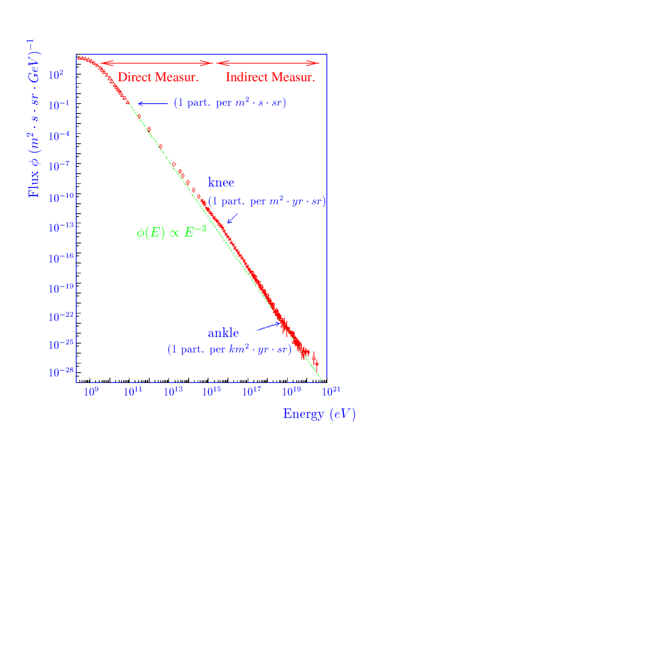
Figure 1.1: All particle cosmic ray energy spectrum. Above are approximately indicated the regions covered by direct and indirect measurements.

At higher energies ($E>$1000 TeV) the flux is too low and one must rely on indirect measurements. In Fig. 1.1 is shown the CR energy spectrum from 1 GeV up to the highest measured energies: in this range the spectrum extends over 10 order of magnitude. To collect a reasonable number of events beyond 1000 TeV, where the flux is of the order of a few particles per year per $m^{2}$, one is forced to build large area detectors at surface level or underground to study secondary particles produced in the interactions of CRs with the air nuclei. Fig. 1.2 show an artist’s view of what happens when a high energy primary CR impinges on an air nucleus. In the first interaction are produced a large number of secondary particle, mainly mesons, which can reinteract or decay in the atmosphere. In particular, $\pi^{o}$ mesons quickly decay in a $\gamma\gamma$ pair to feed the e.m. component of the shower by means of pair production and bremsstrahlung. Large surface arrays of detectors study the “size” of this component counting the number of electrons reaching the detection level. The penetrating component (muons) is generated by the decay of charged mesons, mostly $\pi^{\pm}$ and $K^{\pm}$, into muons ($\pi^{\pm}\rightarrow\mu^{\pm}\nu_{\mu}$ and $K^{\pm}\rightarrow\mu^{\pm}\nu_{\mu}$). The muonic component is the only one that reaches the depths where underground detectors are placed.

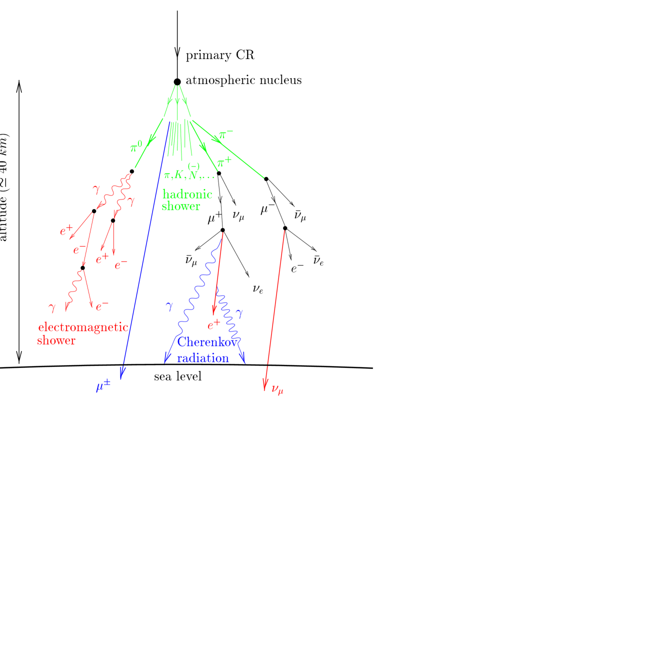
Figure 1.2: Scheme of the shower generation in the collision of a cosmic ray with an atmospheric nucleus.

In this scenario, we understand that indirect measurements require a detailed knowledge of all the physical processes occurring in the interaction and propagation down the atmosphere. In fact, the informations on the chemical composition of primary CR can be extracted on a statistical basis from the comparison between the observations and the results obtained with detailed Monte Carlo simulations. At present, the major contribution on the uncertainties in the interpretation of indirect measurements is the limited knowledge of hadronic interaction models: part of CR interactions occurs in kinematical regions only partially covered by fixed target or collider experiments. Most of the observed particles at sea level or underground comes from the very forward region, where almost all the energy of the interactions is concentrated, allowing the shower penetration down the atmosphere. At present, there is a common effort to provide to the scientific community more and more detailed event generators for the modelling of these interactions.

On the other hand, the problem may be overturned: CR interactions could give us the possibility to investigate the very high energy behaviour of soft interactions in kinematical regions not yet explored at accelerators. In this case, the unknown chemical CR composition prevent us to perform reliable conclusions. We can circuit the problem reducing the “degrees of freedom”, considering observables which are sensitive to a single parameter, the composition model or the hadronic interaction model. The work presented in this thesis is an attempt in this direction in the framework underground muon physics.

In the following we present two different acceleration mechanisms and we show two composition models which find their theoretical explanations in these models. Then we present the results obtained by MACRO in composition studies with the analysis of the multiplicity distribution.

1.2 Acceleration and propagation models

Several hypotheses have been worked out on CR acceleration mechanisms and high energy CR sources. The proposed models have to rest on the following experimental observations:

• the CR all particle spectrum follows a power law of type

  $$\frac{dN}{dE}=KE^{-\gamma}$$ (1.1)

  where the spectral index $\gamma$ is $2.6\div 2.7$ for $E<$ 3000 TeV and is $\sim 3$ above. This changing in the slope is called the “knee” of the spectrum;

• Experimental data extend up $10^{20}$ eV;

We can get information on the nature of the acceleration sources estimating the total power needed to generate CR in our galaxy. The local density of CR in the galaxy is $\rho_{E}\simeq$1 eV/cm³ while the mean living time of CR in the galactic disc is $\tau_{R}\simeq\,6\times\,10^{6}$ years. The needed power to generate all the CR in the galaxy is then

$$L_{CR}=\frac{V_{D}\cdot\rho_{E}}{\tau_{R}}\simeq 5\times 10^{40}erg/sec$$ (1.2)

where the galaxy volume $V_{D}$ is

$$V_{D}=\pi R^{2}d\simeq\pi(15\,kpc)^{2}(200pc)\simeq 4\times 10^{66}cm^{3}$$ (1.3)

A supernova explosion is a good candidate to fit this physical scenario. Supposing to have an acceleration mechanism with an efficiency of some percent, the total CR radiation can be explained by assuming a supernova explosion at a rate of $(30y)^{-1}$ in the whole galaxy. Here we present a model, proposed for the first time by Fermi [2], which explains the acceleration of CRs up to $\sim$ 100 TeV by extensive sources (e.g. the remnant of a supernova explosion).

1.2.1 Acceleration from extensive sources

Let us suppose to have a charged particle of energy $E_{0}$ which enters in a magnetized region of the ISM (Inter Stellar Medium). This particle enter and escapes $n$ times in this region before it escapes definitely, each time gaining an energy fraction $\xi=\Delta E/E$, with $\xi>0$. Let us call $P_{esc}$ the probability of escape from the acceleration region at the end of each of the $n$ acceleration processes. It can be proved [3] that the integral flux of particles with an energy $>E$ is

$$N(>E)\propto\frac{1}{P_{esc}}\left(\frac{E}{E_{0}}\right)^{-\gamma}$$ (1.4)

with $\gamma=\ln\left(\frac{1}{1-P_{esc}}\right)/\ln(1+\xi)\simeq\frac{T_{cycle}}{\xi T_{esc}}$, where $T_{esc}$ and $T_{cycle}=P_{esc}T_{esc}$ are the characteristic times for escape from the acceleration region and for the acceleration cycle respectively. Eq. 1.4 shows that this mechanism naturally leads to a power low spectrum of energies. Moreover, it can be seen that if this mechanism has a limited duration $T_{A}$, it leads to a maximum energy up to which a particle can be accelerated. In fact, if $E_{0}$ is the initial energy of a particle and $n=T_{A}/T_{cycle}$ is the number of elementary accelerations, the maximum energy after a time $T_{esc}$ is

$$E\leq E_{0}(1+\xi)^{{T_{A}}/T_{cycle}}$$ (1.5)

In the case of a supernova blast wave, an estimation of the maximum acceleration energy is

$$E_{max}(GeV)=3\cdot 10^{4}\cdot Z$$ (1.6)

This relation have some consequences on the predicted CR energy spectrum and composition. If the “knee” can be connected to the end-point of the mechanism described, the composition should become progressively enriched in heavier nuclei as energy increases since the maximum energy values are reached by heavy element.

Thus, from this mechanism follows a power law primary spectrum but it limits particle acceleration up to $\sim 100$ TeV. Other models have been proposed to explain particles at higher energies, based on the possibility that the strong magnetic fields close to a few compact astrophysical sources can accelerate particles in limited time scales.

1.2.2 Acceleration from compact sources

Considering that the overall power to generate all CRs with $E\geq 100$ TeV is 1% of the total, we argue that a few highly efficient discrete sources can explain the existence of all high energy CRs. At present, the most favoured candidates are sources connected with a supernova explosion:

1) Let us suppose to have a rotating pulsar with angular frequency $\Omega$ = $\sim 100s^{-1}$, whose magnetic moment has a non zero component perpendicular to the rotation axis $\mu$. This generates a dipole field that can accelerate charged particles. For a pulsar with a typical dimension $\sim$ 10 km and magnetic field at the surface $B\sim 10^{12}$ Gauss the typical power is $\sim 2\times 10^{39}$ erg/sec, which is enough to accelerate particles up to $10^{18}$ eV. In any case, these objects should lose energy at a rate which is in contrast with recents observations. The energy loss from dipole radiation is

$$L=\frac{2}{3}\sin^{2}\theta\frac{\mu^{2}\Omega^{2}}{c^{3}}$$ (1.7)

where $\theta$ is the angle between the rotation axis and the magnetic field. For a typical pulsar with the parameters described above (e.g. Cygnus X-3), the lifetime is $\simeq$ 10 years, a value not compatible with the observation on Cygnus X-3.

2) Another acceleration mechanism takes place in the proximity of a binary system, namely a neutron star and a companion star. In particular circumstances, the matter of the companion star may infall toward the compact object generating an accretion disk composed by ionized particles and therefore a magnetic field opposite to the original one of the neutron star. Between the two opposite edges of the accretion disk arise a potential difference: this accelerates nuclei of the inner edge toward the external edge up to energies $\sim 10^{16}$ eV. The $X$ radiation of the neutron star can have some consequences on the type of CR emerging from the acceleration process: the $\gamma+A\rightarrow n+(A-1)$ process alters the chemical composition of the emitted particles, being this process favoured for heavy nuclei compared to light nuclei. The result is that this CR acceleration mechanism predicts a light component dominating above the knee, in contrast with the prediction of the “leaky box” mechanism.

1.2.3 CR propagation in the ISM

The “knee” in the CR spectrum can be interpreted in different ways. Here we present a propagation model which reconducts the existence of a “knee” to a problem of galactic confinement: the Leaky Box Model. This model associates the galaxy to a box and assumes that particles moving inside it have an escape probability $\tau_{esc}^{-1}<<c/h$ (whit $h$ the semi-thickness of the galaxy), i.e. it assumes that CRs travel distances much larger than the disk of the galaxy during their lifetimes. Neglecting energy losses and inter-particle collisions and assuming a delta-function source term $Q(E,t)=N_{0}(E)\delta(t)$, we can express the number of particles in the galaxy after a time $t$ as

$$N(E,t)=N_{0}(E)e^{-t/\tau_{esc}}$$ (1.8)

A simple interpretation of the parameter $\tau_{esc}$ is the mean time that a particle spends in the galactic volume, while $\lambda_{esc}=\rho\beta c\tau_{esc}$, with $\rho$ $\sim$ 1 H atom/$cm^{3}$ being the mean density of the ISM in the galaxy, is the mean amount of matter crossed by the particle before it escapes from the galaxy and can be parametrised in the form:

$$\lambda_{esc}=10.8\cdot\beta(4/R)^{\delta}\hskip 20.0ptR>4GV$$

$$\lambda_{esc}=10.8\cdot\beta\hskip 60.0ptR<4GV$$

where $R=pc/Ze$ is the rigidity and $\delta\sim$ 0.6. At equilibrium, when $dN/dt$ = 0, the number of primaries of type $i$ in the galaxy is

$$N_{i}(E)=\frac{Q_{i}(E)\cdot\tau_{esc}}{1+\lambda_{esc}/\lambda_{int}}$$ (1.9)

where $Q_{i}(E)$ is the source term and $\lambda_{int}$ is the interaction length. For protons, $\lambda_{int}\sim 55$ $g/cm^{2}$ and, for each energy, $\lambda_{esc}<<\lambda_{int}$. Thus, if the observed spectrum on earth is $N\propto E^{-2.7}$ at high energies, from Eq. 1.9 the source spectrum must be $Q(E)\propto E^{-\alpha}$ with $\alpha\sim 2.1$. On the contrary, for heavy primaries there exists an energy range in which $\lambda_{int}<\lambda_{esc}$. In this range, heavy primaries tend to lose energy more than escape from the galactic volume increasing their overall flux with respect to that of protons.

1.3 Composition at high energy

We have presented some theoretical hypotheses about sources and acceleration mechanisms of high energy CR. We can summarize the results in the following way:
- the existence of the knee in the CR spectrum imposes some constraints on the theoretical interpretation of CR origin;
- the Fermi mechanism applied to supernova shock waves is able to explain the bulk of CR up to $\sim$ 100 TeV;
- there exist several acceleration mechanisms which could explain the existence of CRs of higher energies and the presence of a “knee” in the spectrum.

In this work, we use two composition models which realize the theoretical assumptions just discussed. For each elemental group (H,He,CNO,Mg and Fe) in which CR are usually subdivided, we can express the elemental energy spectrum with

$$\phi_{A}(E)=K_{1}(A)E^{-\gamma_{1}(A)}~{}~{}~{}~{}~{}~{}~{}~{}~{}~{}\rm{for}\it~{}E<E_{cut}(A)$$ (1.10)

$$\phi_{A}(E)=K_{2}(A)E^{-\gamma_{2}(A)}~{}~{}~{}~{}~{}~{}~{}~{}~{}~{}\rm{for}\it~{}E>E_{cut}(A)$$ (1.11)

where the mass dependent parameter $E>E_{cut}(A)$ is the energy cutoff at the “knee” and $K_{2}=K_{1}E_{cut}^{\gamma_{2}-\gamma_{1}}$. Both models must satisfy the requirement that $\sum\phi_{A}(E)$ gives the overall spectrum of Fig. 1.2.

• A “light” model [4]: the model is characterized by the same spectral index $\gamma_{1}$ and the same energy cutoff $E_{cut}$ for all the five components. Beyond 20 TeV the model includes an additional proton component which extends up to the knee, where all the spectral indexes become $\gamma_{1}$ = 3. This composition reflects the assumption of theoretical models with two different acceleration mechanisms, one below and one above the knee.

• An “heavy” model [5]: This model is dominated by the Fe component at high energies: it assumes the same spectral index $\gamma_{1}$=2.71 for all the components with the exception of Fe, which has $\gamma_{1}$=2.36 and a mass dependent cutoff energy $E_{cut}=100\cdot Z\,TeV$. Therefore, the model reflects the physical scenario in which a Fermi mechanism accelerating particles at all energies is coupled with a confinement model as the “leaky box”.

The two model have been adjusted to give the same all particle spectrum [6]. In Tab. 1.1 are reported the parameters of the two models.

LIGHT Mass $K_{1}$ $\gamma_{1}$ $E_{CUT}$ $\gamma_{2}$ Group ($m^{-2}s^{-1}sr^{-1}GeV^{\gamma_{1}-1}$) (GeV) P 1.50$\times 10^{4}$ 2.71 2.0$\times 10^{4}$ 3.0 1.87$\times 10^{3}$ 2.50 3.0$\times 10^{6}$ 3.0 He 5.69$\times 10^{3}$ 2.71 3.0$\times 10^{6}$ 3.0 CNO 3.30$\times 10^{3}$ 2.71 3.0$\times 10^{6}$ 3.0 Mg 2.60$\times 10^{3}$ 2.71 3.0$\times 10^{6}$ 3.0 Fe 3.48$\times 10^{3}$ 2.71 3.0$\times 10^{6}$ 3.0
HEAVY Mass $K_{1}$ $\gamma_{1}$ $E_{CUT}$ $\gamma_{2}$ Group ($m^{-2}s^{-1}sr^{-1}GeV^{\gamma_{1}-1}$) (GeV) P 1.50$\times 10^{4}$ 2.71 1.0$\times 10^{5}$ 3.0 He 5.69$\times 10^{3}$ 2.71 2.0$\times 10^{5}$ 3.0 CNO 3.30$\times 10^{3}$ 2.71 7.0$\times 10^{5}$ 3.0 Mg 2.60$\times 10^{3}$ 2.71 1.2$\times 10^{6}$ 3.0 Fe 3.10$\times 10^{2}$ 2.36 2.7$\times 10^{6}$ 3.0

Table 1.1: Parameters of the “light” model (above) and of the “heavy” model (below). Parameters are defined in Eq. 1.10.

These models have to be considered has “extreme” models, since their high energy behaviour is opposed. In this sense, when applied to the analysis of real data, they should be regarded as trial models to verify the sensitivity of the analysis to the composition models. Anyway, they are more “realistic” than models composed of a single component (only protons or only Fe nuclei), since this possibility is excluded by several experiments.

1.4 The MACRO point of view

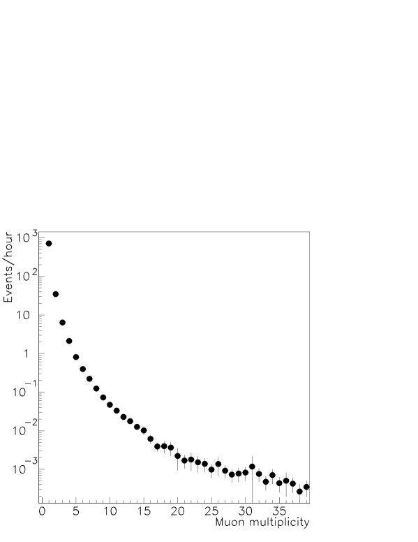
Figure 1.3: Experimental muon multiplicity distributions detected by MACRO. The rate is expressed in events/h.

The muon multiplicity distribution is the observable generally used in underground composition studies. For a recent review of CR composition studies with underground detectors see Ref. [7]. The analysis consists in comparing the experimental multiplicity distribution with the one obtained with Monte Carlo simulations assuming different trial models. This approach has been followed in [8, 9, 10, 11] and, in a first phase, also by the MACRO collaboration [12, 13, 14]. The results, based on a sample of $\sim 2.5\cdot 10^{6}$ muon events, showed that:
1) the MACRO multiplicity distribution is strongly sensitive to the composition model assumed in the simulation;
2) the data prefer a composition model with an average mass number $\langle A\rangle$ flat or slowly increasing with the primary energy and exclude Fe-rich models, (e.g. the “heavy” model), which predict a Fe component asymptotically dominating at high energy.

Fig. 1.3 shows the MACRO experimental multiplicity distributions up to $N_{\mu}$ = 39. In Fig. 1.4 are shown the experimental multiplicity distributions (black point) and those predicted by Monte Carlo simulations using the “light” and “heavy” composition models and the HEMAS Monte Carlo for the hadronic interaction model (see next chapter). The comparison, performed for different rock depths, shows that the “heavy” model is not able to reproduce the data.

A different approach has been followed in [15, 16]. A new procedure, called “direct fit”, has been developed to extract primary CR composition parameters directly from a multi-parametric fit of the experimental distribution. We show here some details of this procedure. The only a priori assumption made on the elemental fluxes is that they have a power law behaviour with the presence of a “knee” (see Eq. 1.10). The underground muon rate $R(N_{\mu})$ can be expressed as

$$R(N_{\mu})=\Omega S\sum_{A}\int dE~{}\phi_{A}(E)\cdot D_{A}(E,N_{\mu})$$ (1.12)

where $\Omega$ is the total solid angle, $S$ is the detection area, $\phi_{A}(E)$ are the fluxes of Eq. 1.10 whose parameters we want to determine and $D_{A}(E,N_{\mu})$ is the probability that a primary CR of mass A and energy E gives $N_{\mu}$ muons detected in MACRO. This probability, computed via Monte Carlo (again using HEMAS), depends on the hadronic composition model, the muon transport into the rock and on detector features. To reduce the number of degrees of freedom in the fitting procedure, the physical assumption on the cut-off energies

$$E_{cut}(Z)=E_{cut}(Fe)\cdot Z/26$$ (1.13)

has been adopted. This corresponds to assume the validity of models which address the existence of the knee to a particle leakage problem in the galactic halo.

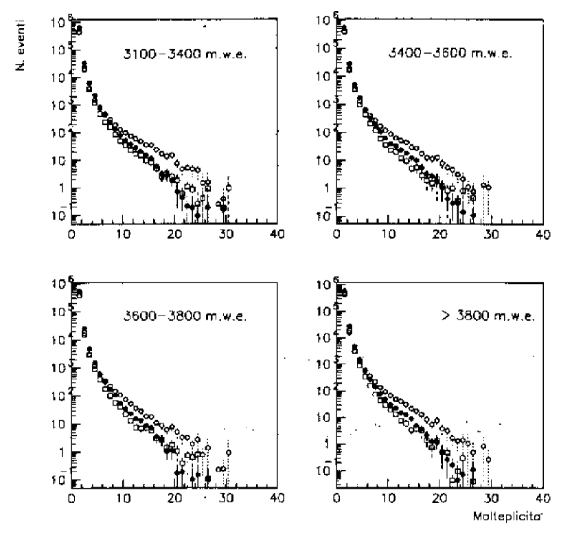
Figure 1.4: Comparison between experimental underground muon multiplicity distributions (black points) and the predictions of the Monte Carlo simulation (open squares: “heavy” model; open circles “light” model. Four different rock-depth windows have been selected.

The function to minimize is

$$\xi^{2}~{}=~{}\lambda_{M}~{}\chi^{2}_{M}~{}+~{}\lambda_{D}~{}\chi^{2}_{D}$$ (1.14)

where

$$\chi^{2}_{M}~{}=~{}\sum_{N_{\mu}}~{}{{[R^{meas}(N_{\mu})-R(N_{\mu}\mid parameters)]^{2}}\over{\sigma^{2}[R^{meas}(N_{\mu})]+\sigma^{2}[R(N_{\mu}\mid parameters)]}}$$ (1.15)

and

$$\chi^{2}_{D}~{}=~{}\sum_{A}~{}\sum^{N_{A}}_{i=1}~{}{{[\phi^{meas}_{A}(E_{i})-\phi_{A}(E_{i}\mid parameters)]^{2}}\over{\sigma^{2}[\phi^{meas}_{A}(E_{i})]}}.$$ (1.16)

$R^{meas}(N_{\mu})$ are the muon rates measured by MACRO (39 experimental points), and $R(N_{\mu}\mid parameters)$ are the predicted muon rates according to formula 1.12. Correspondently, $\phi^{meas}_{A}(E_{i})$ and $\phi_{A}(E_{i}\mid parameters)$ are the experimental fluxes of direct measurements and the ones defined in Eq. 1.10. This technique ensures that the fitting procedure will not to take unphysical values: the weight $\lambda_{M}$ has been fixed to 1, while the weight of direct measurement $\lambda_{D}$ has been changed from 1 to 0.01 in each fitting procedure. The best fit result is obtained with $\lambda_{D}$ = 0.01, corresponding to a $\xi^{2}_{m}in$/n.d.f. = 0.57. The resulting parameters are listed in Tab. 1.2. From now on, we will refer to the model obtained with these parameters as to the “Macro-fit” model.

Mass	$K_{1}$	$\gamma_{1}$	$E_{CUT}$	$\gamma_{2}$
Group	($m^{-2}s^{-1}sr^{-1}GeV^{\gamma_{1}-1}$)		(GeV)
P	1.2$\times 10^{4}$	2.67	2.2$\times 10^{5}$	2.78
He	1.3$\times 10^{3}$	2.47	4.4$\times 10^{5}$	3.13
CNO	3.9$\times 10^{2}$	2.42	1.5$\times 10^{6}$	3.58
Mg	4.5$\times 10^{2}$	2.48	2.6$\times 10^{6}$	3.31
Fe	2.4$\times 10^{3}$	2.67	5.6$\times 10^{6}$	2.46

Table 1.2: Parameters of the MACRO-fit model.

An interesting result of this analysis is that, assuming an asymptotic behaviour for the parameter $E_{cut}(A)\rightarrow\infty$ (i.e. neglecting the existence of the knee) the fitting gives a worse result: $\xi^{2}_{m}in$/n.d.f. $\sim$ 2. The “knee” of the spectrum is observable also underground.

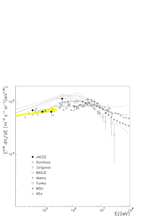
Figure 1.5: All particle spectrum resulting from the MACRO-fit model (solid line) compared to other experimental data (JACEE [17],Danilova [18],Grigorov [19], BASJE [20],Akeno [21],Tunka [22],MSU [23], Tibet AS$\gamma$ [24]) Dashed lines represent $1\sigma$ error. Dashed area represents the spectrum obtained from the fit of direct measurements.

Fig. 1.5 shows the all particle spectrum obtained with this analysis compared with the ones of other direct and indirect measurement. The striking result is that the agreement with high energy indirect measurements is good, while in the region covered by direct measurement the agreement is lost: at $E\sim$ 100 TeV, the discrepancy is about 50%.

Figure 1.6: Energy spectra for each mass group resulting from the MACRO-fit model superimposed to direct measurement data. The solid line is the MACRO-fit, the dashed lines the $1\sigma$ limits. Full circle: JACEE [17], full triangle [25], open squares: CRN [26].

From Fig. 1.6 we understand that this mismatch is due to the light components (H and He) of CR spectrum, while for heavier elements the agreement is good. From these results, one can draw two conclusions:
1) Either the systematics in this procedure is not well under control, mainly because of uncertainties connected with the modelling of the high energy hadronic and nuclear interactions;
2) Or the procedure to estimate the light primary CR fluxes with direct measurements is not completely correct.

Point 1) is under study. The analysis presented in [27] used the DPMJET hadronic interaction model interfaced with HEMAS (see Chapt.3) to estimate the quantities $D_{A}(E,N_{\mu})$ in Eq. 1.12. Even if the analysis has been performed in a limited angular window of rock depth and zenithal angle, the results show that the mismatch between direct measurements and the fit of MACRO data is reduced.

This topic addresses a more general and fundamental problem of CR physics, which we have mentioned at the beginning of this Section. We study CR’s composition in the “knee” region to throw light on high energy phenomena occurring in our galaxy and in the whole universe. On the other hand, this study strongly relies on the knowledge of high energy hadronic interactions, since the measurements are of indirect nature. In this framework hadronic interactions are the “manifestation” of QCD in regions not yet explored at colliders and their study with CRs require the knowledge of CR composition. A complete a definitive solution of this “puzzle” can be obtained only considering the whole set of experimental data at disposal of the scientific community. An ambitious program suggests to resolve the problem looking at CR physics from different “point of views”: considering all the data coming from high and medium altitude, surface, shallow depth and underground experiments we could analyse them in a sort of multivariate analysis. The result must be self-consistent, i.e. it must satisfy each of the “point of view” which compose the set of data. In this context, it is clear that each specific analysis made by a single experiment can be crucial when inserted into the complete set of experimental data. Part of this work (Chapter 4) is intended to prove that the transverse structure of hadronic interactions in the energy region of the bulk of MACRO data ($\sim 20$ TeV up to the “knee”) is well reproduced by the HEMAS Monte Carlo code. In the second part (Chapter 5), we are going to analyse high multiplicity events and hence the high energy part of MACRO data (above the “knee”) using alternative analysis methods and comparing the results with the predictions of different hadronic interaction models.

Chapter 2 The MACRO experiment

2.1 Generalities

The MACRO experiment (Monopole, Astrophysics and Cosmic Ray Observatory) is located in the hall B of the Gran Sasso underground Laboratory (see Fig. 2.1) in Central Italy at 963 m a.s.l. The average overburden of calcareous rock is $h\sim$ 3700 $hg/cm^{2}$; the minimum overburden is $h\sim$ 3100 $hg/cm^{2}$ corresponding to a muon threshold energy $E^{thr}_{\mu}\sim$ 1.4 TeV. At the average depth of the Laboratories, the muon flux reduction factor is $\sim$ $10^{-6}$.

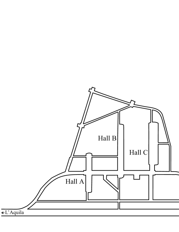
Figure 2.1: Map of the tunnel system of the underground Laboratories. The MACRO experiment is located in the Hall B of the Gran Sasso Laboratories.

The main aims of the experiment are the search for GUT Magnetic Monopoles, the study of cosmic rays, the study of atmospheric neutrinos and the search for neutrinos from stellar collapses. The apparatus is composed of three different and complementary “sub-detectors”: a system of limited streamer tubes chambers is used for particle tracking, the particle timing is realized by means of liquid scintillation counters, nuclear track detector acts as an independent system for rare particle searches. The three sub-detectors allow to have redundant informations in the framework of rare process physics where one expects few events in the whole life time of the experiment.

The large acceptance ($\sim 9600$ $m^{2}sr$ for an isotropic flux of particles) and the long life time of the experiment (MACRO started data taking on 1989 February and it is planned to run at least up to the end of year 2000) allowed the collection of a large amount of data: $\sim 4\times 10^{7}$ muon events, of which $\sim 5\%$ are multiple muons.

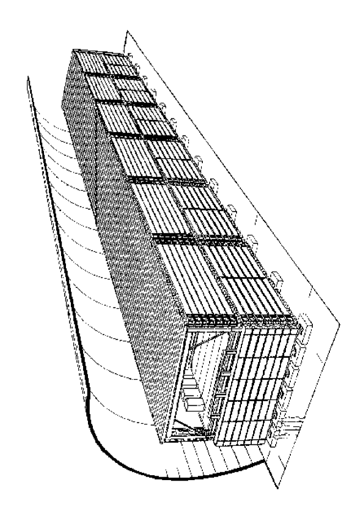
Figure 2.2: Artist’s view of the MACRO Detector.

2.2 Detector description

The MACRO detector [28] is arranged in a modular structure of six supermodules (Fig. 2.2). Each of these is 12 m$\times$12 m$\times$9 m in size and consists of a 4.8 m lower part and a 4.2 m upper part, the “attico”. This modularity ensures the continuity of data taking allowing parts of the detector to be shut off for maintenance. In the lower part, each supermodule is composed by two central modules and two lateral walls (east and west) which run over the long side of the detector. Two end-caps close the apparatus (north and south). The “attico” has a different structure: it consists of two vertical walls along the longer side of the detector, without endcaps, and a “roof” which covers the whole length of the apparatus; there thus is an empty space where the electronics is placed.

2.2.1 The Streamer Tube System

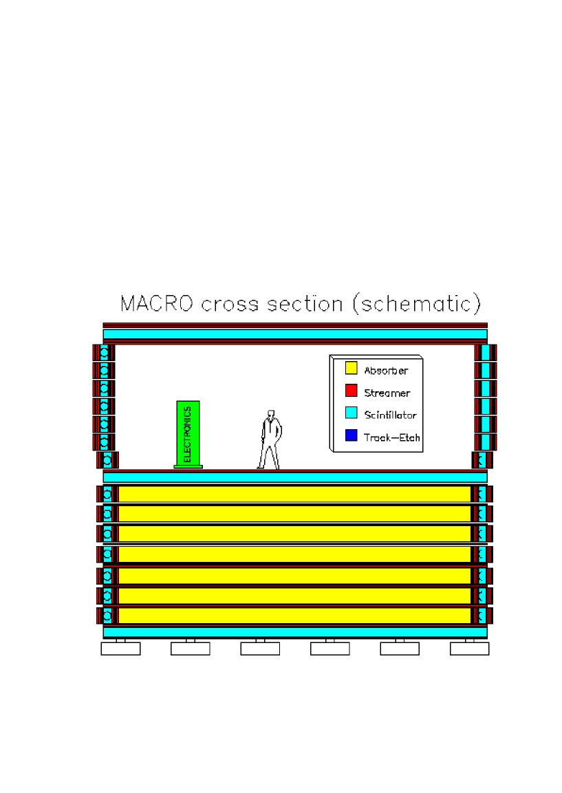
Figure 2.3: Section of the MACRO Detector.

In the lower part, the limited streamer tubes are distributed in ten horizontal planes separated by $\sim$ 60 g cm^-2 of CaCO₃ (limestone rock) absorber, and in six planes along each vertical wall. In the attico, four planes are disposed in the horizontal part (the roof) and six planes in the vertical walls (Fig. 2.3). From each horizontal plane of the lower part two coordinates are provided, the wire (perpendicular to the long detector dimension) and strip views. These second view uses 3 cm wide aluminium strips at 26.5^∘ to the wire view. In the attico also the vertical walls are provided with strips, at 90^∘ with respect to the wire view. The average efficiencies of the streamer tube and strip systems are 94.9% and 88.2%, respectively. Fig. 2.4 shows an eight-cell chamber.

The spatial resolution achieved with this configuration depends on the granularity of the projective views. The average width of a cluster, defined as a group of contiguous muon ”hits,” is 4.5 cm and 8.96 cm for the wire and strip views, respectively. Muon track recognition is performed by an algorithm which requires a minimum number of aligned clusters (usually 4) through which a straight line is fitted. The differences between the cluster centers and the fit determine a spatial resolution of $\sigma_{W}$=1.1 cm for the wire view and $\sigma_{S}$=1.6 cm for the strip view. These resolutions correspond to an intrinsic angular resolution of $0.2^{0}$ for tracks crossing ten horizontal planes. This angular resolution must be compared with the angular resolution due to Coulomb multiple scattering in the rock. This value can be extracted from the dimuon angular separation distribution. Fig. 2.5 shows the 3D angular separation between muon pairs with and without the attico. The $1\sigma$ integral of the distribution is at $1.3^{\circ}$ and $1.0^{\circ}$ for the case without and with the attico, respectively; they correspond to an intrinsic angular resolution of $1.3/\sqrt{2}=0.92^{\circ}$ and $0.70^{\circ}$, respectively.

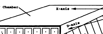
Figure 2.4: Cross section of a eight-cell chamber of limited streamer tubes. Under the uncoated surface of the chamber, the system of aluminium strips is placed.

The elemental unit of the streamer tube system is a chamber (Fig. 2.4) of dimension 3.2 cm$\times$25 cm$\times$12 m each one composed of eight cell of dimension 2.7 cm$\times$2.9 cm. In each horizontal plane are placed 24 chambers, 14 in the vertical walls for a total number of 6192 chambers in the whole detector (corresponding to 49536 wires). Three of the four internal sides of each cell are coated with low resistivity graphite ($<$ 1 $k\Omega/square$) which acts as cathode, while the anode is a silvered Be-Cu wire 12 m long and with a diameter of 100 $\mu m$, disposed in the center of the cell. The whole chamber is enveloped in a PVC container. The gas mixture used is 73% He and 27% n-pentane, studied to exploit the Drell-Penning effect [29] for slow monopole detection. The total gas volume in the all active elements of MACRO is about 465 $m^{3}$ and a continuous recirculation ensures a “good quality” of the gas. When a charged particle crosses a cell, electrons that are stripped from the gas molecules migrate toward the wire (anode). The particular choice of the wire diameter and of the gas mixture allows a single electron to produce an avalanche. This is due to the high electric field near the anode, since the electric potential goes as $log(r)$. The freed electrons and secondary photons produce the avalanche of secondary electrons which proceeds as a column towards the cathode walls producing the streamer. The ultraviolet photons may be absorbed by the gas if a particular mixture is chosen, so to limit the streamer formation near the cathode. The HV working point can be determined by monitoring the single rate plateau from a $\beta$ source. The starting point of the plateau is at $\sim$ 4200 V and it has an average width of $\sim$ 700 V. The drift time of the streamer inside a cell has a triangular distribution with a maximum value of $\sim$ 600 ns and an average value of $\sim$ 150 ns which is the timing resolution.

The readout of each chamber is provided by an eight channel card, 14 cm large, directly connected to the HV with a 16 pin connector. The analog signal is amplified and discriminated (V$>$40 mV on 330 $\Omega$) and sent to a ADC/TDC system (QTP modules) and to the trigger electronics. The output is a TTL signal with pulse width 10 $\mu$s for fast particles and 550 $\mu$s for slow particles and sent to shift register (FAST and SLOW chain respectively). The informations contained in these registers are sent to the Streamer Tube Acquisition System (STAS) by means of dedicated electronic modules called splitter boards. The tube wire readout card provides also the OR of TTL signals and additional digital OR (DigOR) from all the wires in the 12m x 12m area of each plane. The strips readout cards read each one a group of 32 strips. Each card contains an hybrid D779 CMOS integrated circuit which amplify and discriminate the signal. A 4.43 MHz clock determines the width of the output signal which is shaped at 600 $\mu$s for the slow chain and 14$\mu$s for the fast chain.

Streamer tube triggers
A simple trigger classification can be made on the basis of particle velocity.

For fast particles, the triggering system is based on EPROM components, in which are codified the triggering conditions. Three EPROMs are used: one for signals coming from horizontal planes, one for signals coming from vertical planes and one for mixed cases (horizontal and vertical). The EPROM input is the OR of the discriminated signals coming from each horizontal plane or from each vertical plane of each supermodule. The triggering conditions are:
- 6/10 horizontal planes in coincidence;
- 5/10 contiguous horizontal planes in coincidence (excluded the first and the last plane);
- 3/10 horizontal and 3/6 vertical East in coincidence;
- 3/10 horizontal and 3/6 vertical West in coincidence;
- 3/6 vertical East and 3/6 vertical West in coincidence;
- 5/6 vertical East in coincidence;
- 5/6 vertical West in coincidence;

The main purpose of slow particles triggers is to distinguish a slow monopole from random background signals ($\sim$ 40 Hz/$m^{2}$) occurring during the long gate time of the slow chain. Since the streamer tube system is a low noise device, the only background is due to local radioactivity, that in MACRO is $\sim$ 40 $Hz/m^{2}$. The background signals are generated in random positions and times in contrast with what one expects from the passage of a massive slow monopole. Thus, the triggering conditions requires the spatial and time alignment of the hits. In particular, for horizontal planes is only required the time alignment of 6/10 planes; for vertical planes the trigger requires also spatially aligned hits, since the time of flight in a vertical wall is very short.

Figure 2.5: Distribution of the angular separation of dimuons with the attico (dotted lined) and without (solid histogram).

2.2.2 The Scintillator System

The main purposes of the MACRO scintillator system are:
1) Measure the energy loss $dE/dX$;
2) Measure the velocity and versus of penetrating particles time of flight;
3) Detection of bursts of low energy $\bar{\nu}_{e}$ from gravitational collapses.
In each supermodule, 32 horizontal and 21 vertical counters are placed in the lower part of the detector while 16 horizontal and 14 vertical counters are placed in the attico. Each counter is a box of dimension 12m$\times$50cm$\times$25cm and is filled with liquid scintillator: in total, the apparatus consists of 476 scintillator counters for a total amount of $\sim$ 600 tons of liquid scintillator. The composition of the scintillation mix is:
- 96.4% of high purity mineral oil base with a nominal attenuation length $\sim$ 20 m at a wave length $\lambda$ = 425 nm;
- 3.6% pseudocumene;
- 1.44 g/l PPO;
- 1.44 mg/l bis-MSB;
The density of this mixture is 0.85 $g/cm^{2}$ and the attenuation length is $\sim$ 12 m. Each scintillator box is divided into three chambers separated by transparent PVC windows: the larger is the middle one ($\sim$ 11m) which is filled with the liquid scintillator; the other two, placed at the two box ends, contain the PMT and are filled with the same mineral oil of the middle chamber to ensure a good optical coupling (the optical transmission is $>$ 90% for wavelength $>$ 400 nm). This geometry allows the rejection of spurious signals near the PMT coming from natural radioactivity. The inner walls of the middle chamber are lined with a vinyl-FEP material, with a refractive index of 1.33 to be compared to the refractive index of the liquid scintillator of 1.47. In this way, the critical angle for total reflection is 25.6^∘. Total reflection is also provided by the air/scintillator liquid interface in the middle chamber.

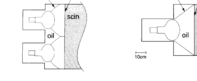
Figure 2.6: Geometry of the horizontal (left) and vertical (right) counters, and optical coupling between the end chambers and central ones. The active liquid scintillator volume is 11.20 m for the horizontal counters and 11.07 m for the vertical ones.

Each end of the horizontal counters has two PMTs (Fig. 2.6) of type EMI D-642 while vertical counters have a single PMT at each end (vertical counters of the attico are of type Hamamatsu R-1408). These are hemispherical PMTs with a photocathode of dimension $\sim$ 20 cm and 14 dynodes (13 in the Hamamatsu) disposed in a venetian blind structure. The typical gain for a single photo-electron is $\sim$ 10⁷ corresponding to a pulse height of 3 mV. The used HV is about -1500 V: 550 V between the photocathode and the first dynode and the remaining 950 uniformly distributed between the other dynodes.

The monitoring of the scintillator system is performed by means LEDs mounted in the end chambers near the PMTs and UV light from N laser coupled to the scintillator liquid with optical fibres. Calibrations are performed periodically (once per week) and every four hours to on line verify the performance of the data taking. At four hour intervals during the data taking, each LED simulate the passage of different particle types, varying the light pulses, and are able to excite single photoelectron signals. In the calibration with N laser pulses all the counters are illuminated simultaneously. Another calibration technique consists in analysing single muon events using the informations from the tracks reconstructed by the streamer tube system.

Considering the difference of arrival time at each counter end, it is possible to estimate the position in the scintillator of the crossing particle. The difference between this value and the one obtained with the streamer tube system can be used to estimate the spatial resolution of the scintillator system. The standard deviation of the distribution of the difference is $\simeq 11$ cm corresponding to a time resolution for the single counter $\simeq 520ps$. Therefore, the time resolution on the time of flight measurement is

$$\sigma_{TOF}\simeq\sqrt{2}\cdot 520ps\simeq 750ps.$$

This result is used in MACRO to discriminate the arrival direction of relativistic particles and to tag upward neutrino-induced muons.

Scintillator triggers
- CSPAM: this trigger considers each lateral wall as a unique “supercounter” and takes in input the two signals generated by the sum of each PMT in the two “supercounter” ends. The two signals are compared and if they are in a 100 $ns$ windows with a minimum amplitude of 200 $\mu$V, a pretrigger signal is generated. If two opposite walls generate a pre-trigger in a 1 $\mu$sec window, a trigger signal is generated. - ERP: this trigger reconstructs the energy loss by muons in the scintillator tanks and provides the crossing time. The signals at the two PMTs are compared with the ones contained in RAM look-up tables (LUT). For each pair of signals, the corresponding energy is computed and if it exceeds a threshold value of 10 MeV, the trigger is generated.
- FMT: this trigger uses the same CSPAM electronics, but it requires a time window of 10 $\mu$sec and operates in anti-coincidence with CSPAM.
- PHRASE: the purpose of this trigger is the search for $\bar{\nu}_{e}$ of energy $\sim$ 10 MeV from gravitational collapses by means the CC reaction $\bar{\nu}_{e}+p\rightarrow n+e^{+}$ with the protons of the scintillator. The threshold for the positron detection is 5 MeV; when a trigger condition occurs the threshold is lowered to 1 MeV for 850 $\mu$sec to detect the photon (with energy $E_{\gamma}\sim$ 2.2 MeV) following the neutron capture: $n+p\rightarrow d+\gamma$.
- TOHM (SMT): the analog signals from PMT anodes are converted into TTL signals whose duration is nominally the time that the input pulse is larger than its half height. This circuit is studied to suppress large and sharp pulses produced by muons and natural radioactivity. A circuit (Leaky Integrator) takes in input and integrates the TOHM output, giving a wide signal if the input is a wide pulse or a dense burst of single photoelectrons in the case of slow monopoles.
- LaMoSsKa: The main purpose of this trigger is to provide an early stop to WFDs for high energy events. It takes the input from the CSPAM “supercounters”: the signals are discriminated and 110 $\mu$sec delayed before to sent the stop to WFDs.
- St-Sc trigger: this a “mixed” trigger since it uses both the informations of streamer tube system and scintillator system. In presence of a slow (central or lateral) monopole trigger with the streamer tube system, the WFDs of the corresponding modules are read (central or lateral respectively).

2.2.3 The track etch detector

The main purpose of the track-etch detector is the search for magnetic monopoles. This detector is organized in “trains” each one containing 47 “wagons” of 25$\times$25 cm² in size. A “wagon” contains three layers of CR39 (1.4 mm thick), a layer of aluminium absorber (1 mm thick) and three layer of LEXAN (0.2 mm thick) as is shown in Fig. 2.7. The detector is placed on the vertical walls on the east and north sites and horizontally in the middle of the lower apparatus. The passage of a highly ionizing particle causes damages in the polymeric structure of the materials and they can be amplified by chemical etching the plastic layers. The etching of the first sheet is performed in a solution 8N of NaOH at $80^{\circ}$ C. The layer is analysed by means of a binocular optical microscope; if a candidate is found, we etche a second layer in a “normal” etching in a solution 6N of NaOH at at $70^{\circ}$ C.

This detector can be used as a stand alone detector, as a passive detector, or can be used in coincidence with the other MACRO detection sub-systems. When a “candidate” is triggered by the scintillation counters or by the streamer tube systems, the corresponding “wagon” around the expected position can be extracted and analysed.

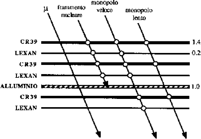
Figure 2.7: Layout of the track-etch detector.

2.3 The MACRO Data Acquisition System

The MACRO Data Acquisition System (DAS) is based on a network of KAV 30 Vax Processors and MicroVAX II supported by a VME and CAMAC system crates. The system has been upgraded after a first period in which the MACRO DAS was based only an a network of MicroVAX IIs to include VME front-end electronics of the new Wave Form Digitizers [30] for the scintillator counters. The system runs under VAXELN, a dedicated operating system of VAX computers developed by DIGITAL to have an high I/O speed ($\sim 300$ kbyte/sec). The KAV30 processors are located in VME crates, which act as “Master Crates” from which remote VME and CAMAC crated may be accessed.

Figure 2.8: General layout of the MACRO Data Acquisition System.

In Fig. 2.8 it is shown a general layout of MACRO DAS. The three KAV30 processors control a supermodule pair each one, while the three MicroVAX-IIs control the PHRASE trigger of the scintillators for the monitoring of stellar collapses. A central VAX 4000/500 running under VAX/VMS performs the data logging and is used as interface from the user to the MACRO DAS. All the computers are connected vis Ethernet/DECNET and a DEC bridge connects the MACRO LAN (Local Area Network) to the LNGS LAN of outside Laboratories. The LNGS LAN is composed by segments connected by optical fibres covering the 6 km which divide the external from the internal Laboratories. From outside, the user can connect to the MACRO LAN and copy raw data files or submit directives to execute CAMAC operations. The timing in MACRO is performed by means the LNGS atomic clock, syncronized with the UTC/USNO standard using the satellitar GPS system. Each second the GPS system transmits a signal containing satellite status and timing to a “Master Clock” located on the outside Laboratories. This generates the local time with a 10 MHz signal using a rubidium oscillator and drives a set of six “Slave Clocks” located underground near the apparatus which corrects the signal and reproduce the UTC/USNO time with an accuracy of $\sim$ 100 ns.

2.4 Off-line analysis

Event recorded in the central VAXes are reprocessed and copied in a multi-run tape in an machine independent format. This operation is accomplished by DREAM (Data Reduction and Event Analysis for MACRO), a dedicated code which perform the event decoding and event reconstruction of MACRO events. The code is structured in “passes”: the pass 0 is the I/O procedure just described which rewrites data in a machine independent format. Pass 1 corresponds to the event decoding while pass 2 reconstructs the relevant physical parameters of an event. Finally, pass 3 provide the complete event reconstruction, including the number of tracks in the event and their position in the absolute frame of the detector. DREAM is written in standard FORTRAN 77 and uses software packages from the CERN libraries, so that it can be used by other machines.

The main informations contained in the output of pass 3 are written in DST files (Data Summary Tape). This operation preserves all the relevant parameters of the event performing a data reduction of a factor $\sim 60$.

Chapter 3 Monte Carlo simulation

3.1 Introduction

The Monte Carlo simulation is a crucial point in underground muon physics, where many measurements are of indirect nature. The comparison between experimental and simulated data requires a detailed knowledge of all physical processes occurring during the shower development (in particular the modelling of hadron-air interactions) and requires a correct treatment of energy losses and stochastic processes of TeV muons in the rock overburden. Finally, a detector simulator which reproduces data in the same format of experimental one is required. We will refer to the MC codes which model the development of the shower in atmosphere as shower propagation codes, to distinguish them from the MC implementation of nuclear and hadronic interaction models which we shall call event generators. All the software packages which separately describe these steps are interfaced one to an other. For instance, the implementation of a given hadronic interaction model can be easily included in a shower propagation code without altering the general structure of the program. In the following we are going to examine in detail all the steps that form the MC simulation chain.

3.2 Shower propagation codes

A shower propagation code should take into account all physical processes which occur in atmosphere: computation of the first interaction point of primary cosmic rays on the basis of the input cross sections, propagation of the e.m. and hadronic components of the shower considering the actual mean free path of particles, deflection of charged particles by the geomagnetic field. Fundamental parameters of the simulation are the threshold energies down to which the particles in the atmosphere must be followed: the CPU time required to follow particles of ever decreasing threshold energies quickly diverges. Since this work concerns the study of TeV muons, we can introduce the approximation of a sharp cut of $E_{min}$ = 1 TeV in the atmosphere because the probability that a muon generated from the decay of a parent meson with energy $E_{meson}<1$ TeV survive at Gran Sasso depth is negligible.

In this work we use two different shower propagation codes: HEMAS [31] and CORSIKA [32].

3.2.1 HEMAS

HEMAS [31] (Hadronic, Electromagnetic and Muonic components in Air Showers) was originally designed as a fast tool for the production and propagation of air showers. It allows the calculation of hadronic and muonic components of air showers above 500 GeV and e.m. shower size above 500 KeV. In its first version [31], the interaction and decay processes were simulated only for $\pi,K$ and $N$ primaries. Neutrinos are produced in the decay routine, but they are not followed in the shower. In the updated version we used [33, 34], many other secondary particles may be followed in atmosphere, including primary nuclei. In this version the user can select two different interaction models: the original HEMAS [31] and DPMJET [35]. When the DPMJET model is selected, prompt muons from D meson decay are generated too. In HEMAS, the mean free paths in atmosphere are related to inelastic cross sections of primary cosmic rays. For the nucleon we have

$$\lambda_{p-air}(g/cm^{2})=\frac{2.4\times 10^{4}}{\sigma_{p-air}(mb)}$$ (3.1)

and similar relations for other primaries or produced hadrons. Three different options are provided for nuclei initiated showers ($A>1$):

• Superposition model: here the development of a shower initiated by a nucleus of mass A and total energy $E$ is considered equivalent to A sub-showers initiated by A independent nucleons each one of energy $E/A$. The atmospheric depth of the first $p-Air$ interaction follows a relation of this type [3]

  $$\frac{dP_{I}}{dX}=\exp[-X/\lambda_{N}]$$ (3.2)

  where $X$ is the atmospheric depth (in $g/cm^{2}$) and $\lambda_{N}$ is the nucleon interaction length ($\sim 80\,g/cm^{2}$). This approach is quite unrealistic because it assumes that the cross section of proton and heavy primaries are the same. In any case, this simple approximation well reproduces the average quantities of a cosmic ray shower, even if it dramatically underestimates the fluctuations around their average values.

• A more realistic model is the so called semi-superposition model [36]. Here the shower is again the result of A independent sub-showers, but the first interaction points of these interactions are computed in a more realistic way. The number of inelastic collisions between projectile nucleons and target nucleons are computed in the framework of the Glauber formalism [37]. Let us consider the collision of a projectile nucleus of mass $B$ with a target nucleus of mass $A$. If we call $P_{ij}$ the probability of an inelastic collision between a nucleon $i$ of the projectile and a nucleon $j$ of the target (function of the impact parameter of the two nuclei configuration) we can express the total cross section of the two nuclei as

  $$\sigma_{AB}=\int{d^{2}b}\int{[dr_{A}]}\int{[dr_{B}]}\{1-\prod_{i=1}^{A}\prod_{j=1}^{B}\,[1-P_{ij}]$$ (3.3)

  where $[dr]$ indicates the integral over the configuration of the nucleus A. In general, the average number of nucleon-nucleon interaction in the collision of the two nuclei is expressed by

  $$<\!N\!>=\frac{AB\sigma_{pp}}{\sigma_{AB}}$$ (3.4)

  where $\sigma_{pp}$ is the proton-proton cross section and $\sigma_{AB}$ is the cross section of the two nuclei $A$ and $B$ computed with Eq. 3.3.

• Direct interaction. This option (which can be used only with the DPMJET model) simulates the nuclear interaction without approximating it to a set of nucleon-nucleus interactions, but it takes into account all the nuclear processes involving a nucleus-nucleus interaction. This option will be described in detail in a dedicated section.
  

HEMAS neglects the muon energy loss in atmosphere, since this contribution is negligible for muons detected underground. The muon threshold energy at production to reach the surface level is $\sim 2$ GeV and this value must be compared to the typical energy of muons which reach the underground detectors level (1 TeV). The geomagnetic deflection is taken into account for muons, but is neglected for charged hadrons, being their mean free path too short to produce observable effects underground.

In HEMAS two different atmospheric profiles can be chosen: the first is a parametrization of the atmosphere at the Gran Sasso location in Central Italy and the second corresponds to the USA Standard Atmosphere according to the Shibata’s fit [3].

All these options can be switched on and off by the user.

3.2.2 CORSIKA

CORSIKA [32] (COsmic Ray SImulation for KAscade) is a shower propagation code originally developed for the KASKADE experiment, but it is now become one of the standard tools in cosmic ray physics. The computation of the mean free path in atmosphere, the interaction probabilities and the deflection of charged particles in the geomagnetic field are computed similarly to HEMAS. Being CORSIKA designed for experiments at sea level, it takes into account ionization energy losses and multiple coulomb scatterings of charged particles in atmosphere. Also in this code the user can select the desired atmospheric profile.

CORSIKA is interfaced with different high energy hadronic interaction codes: DPMJET, HDPM, QGSJET, SIBYLL and VENUS. These models will be described in the following section. The simulations of low energy hadronic interactions are performed with GHEISHA [38] or ISOBAR [39] codes.

3.3 Interaction models and Monte Carlo implementation

3.3.1 Theoretical framework

High energy hadronic interactions are dominated by the inelastic cross section with the production of a large number of particles (multiparticle production). Most events consist of particles with small transverse momentum $p_{t}$ with respect to the collision axis (soft production), while a small fraction of events results in central collisions between elementary constituents and produce particles at large $p_{t}$ (hard production). QCD (which is the now accepted theory for strong interactions) is able to compute the properties of hard interactions: here the momentum transfer between the constituents is large enough (and the running coupling constant is small enough) to apply the ordinary perturbative theory. On the other hand, soft multiparticle production is characterized by small momentum transfer and one is forced to build models and adopt alternative non-perturbative approaches. Several models have been developed during the years: here we remind the Dual Parton Model (DPM) [40], developed at Orsay in 1979, and the Quark Gluon String model (QGS) [41], developed at ITEP (Moscow) during the same years. These two models, equivalent in many aspects, incorporate partonic ideas and QCD concepts (as the confinement) into an unitarization scheme to include hard and soft components into the same framework. We will return in the following to give a more detailed description of these models.

The lack of a detailed theoretical description of soft hadronic physics is coupled with the lack of experimental data for these processes. The knowledge of the properties of high energy hadronic interactions mainly derives from experiments at accelerators or colliders. Here best studied is the central rapidity region, populated by particles hard scattered in the collisions. In the (target or projectile) fragmentation regions we find particles produced at small angles which escape into the beam pipe and hence they are not observed.

The point is that, for the development of a CR shower, particles produced in the fragmentation region are the most important since they are the ones that carry the energy down the atmosphere and produce the “bulk” of secondary CRs observed on Earth. In fact, most of the CR collisions are peripherals, with large impact parameters and consequently small momentum transfer. It seems clear that the modelling of high energy hadronic interactions for CR studies has to deal with different problems:

• In CR interactions, part of the c.m. energy for hadron-hadron collisions extends above the actual possibilities of collider machines. Experimental data extends up to $\sqrt{s}=63$ GeV for $pp$ interactions (ISR) and up to $\sqrt{s}=1.8$ TeV for $p\bar{p}$ interactions (Tevatron). Thus one is forced to extrapolate these measurements into regions not yet covered by collider data.

• The kinematical regions of interest for CR physics (and underground muon physics) is the one of projectile fragmentation; here data from colliders extends up $\eta\sim$ 5.

• Part of CR collisions in atmosphere are nucleus-nucleus collisions. In this case, the data from fixed target experiments extends only up to few GeV/nucleus is the laboratory frame.

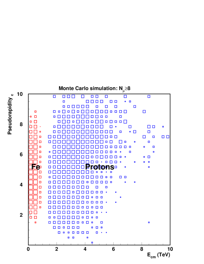
Figure 3.1: Kinematical region of the nucleon-nucleon interactions which produce high multiplicity muon bundles ($N_{\mu}\geq 8$) at Gran Sasso depth. The role of iron and proton primaries is separated.

This situation is summarized in Fig. 3.1: we used a Monte Carlo simulation (with the DPMJET interaction model) to compute the kinematical regions of high energy CR interactions which produce high multiplicity muon events observed at Gran Sasso depth (event multiplicity $N_{\mu}\geq 8$). We plot the pseudorapidity $\eta_{cm}$ of the produced mesons (parents of underground muons) versus the nucleon-nucleon c.m. energy $E_{cm}$. We separate the contribution of protons and iron primaries: iron primary collisions are still far from the c.m. energy/nucleon values reached in heavy ion collision experiments and, in the case of protons, more than half of the collisions have $E_{cm}>1.8$ TeV and $\eta_{cm}>5$.

We understand now why the role of the interaction model in CR physics is at present the major contribution to systematic uncertainties. Experimental data from collider can be used to built hadronic interaction generators in the following way:
- data can be used to tune and check generators built on the basis of physically inspired models (as DPM or QGS). These generators contain a detailed description of the interaction processes, starting from elementary collisions between partons inside the projectile and target. The requirement is that these generators must reproduce the properties of hadronic interactions in kinematical regions where data already exist.
- an alternative (and less realistic) approach is to build a generator directly from the parametrizations of the most important features of hadronic interactions, extrapolating them in kinematical regions not yet explored. Most of the properties of the interactions at low energy (where data exist) are obtained “by construction”. In any case, this treatment of the hadronic interactions is approximate since the extrapolation to higher energies is subject to large uncertainties and many of the correlations existing between final state particles may be lost.

A general feature of high energy hadronic interactions is the rise with the c.m. energy $\sqrt{s}$ of many of the exclusive and inclusive variables which characterize these reactions. For instance, if we define (at fixed energy) the global transverse momentum

$$\langle P_{t}\rangle=\frac{1}{N}\sum_{i=1}^{N}\sum_{j=1}^{m_{i}}|p_{t}^{ij}|$$ (3.5)

where $i$ runs over the events and $j$ runs over the particles of the $i$-th event of multiplicity $m_{i}$, it has been found experimentally that $\langle P_{t}\rangle$ grows logarithmically with the energy. For instance, $\langle P_{t}\rangle$ = 350 MeV/c at $\sqrt{s}$ = 63 GeV (ISR) and $\langle P_{t}\rangle$ = 500 MeV/c at $\sqrt{s}$ = 1.8 TeV (Tevatron). The inclusive $p_{t}$ distributions are well fitted by power law functions

$$\frac{d\sigma}{dp_{t}^{2}}=const\left(\frac{p_{0}}{p_{0}+p_{t}}\right)^{n}$$ (3.6)

for $p_{t}>$ 1.5 GeV, while at lower values it is well interpolated by an exponential distribution.

The average charged multiplicity distribution can be described by a function of the type

$$\langle N_{ch}\rangle=A+B\cdot lns+C\cdot ln^{2}s.$$ (3.7)

This result is one of the manifestations of the Feynman scaling breaking: under the hypothesis of complete scaling (i.e. the total cross section depending from the energy only through a function of $x_{F}\equiv 2p_{l}/\sqrt{s}$), Eq. 3.7 should hold with C = 0.

Another experimental observation of the Feynman scaling breaking is connected with the height rise with the energy of the rapidity plateau. This is the kinematical region populated by the hadronization of hard scattered particles and include the contribution of gluon and sea quarks. The plateau ends, where the distribution is quickly decreasing, are populated by the hadronization of particles coming from the valence quark chains and leading hadrons. Feynman postulated that the height of the plateau is energy independent: again, high energy data show that this is an approximation valid only at low energies. The scaling violation of the fragmentation region, if exists, is very small and should be connected with the leading hadrons.

An experimental evidence that Monte Carlo generators must take into account is the existence of “minijet” in high energy data. The UA1 collaboration [42], analysing minimum bias events, found that part of these events were formed by jets of particles with small $p_{t}$ if compared to the typical QCD multijet events. Events containing jets with a transverse momentum $p_{t}>5$ GeV made up one-third of the cross section. These jets are fed mainly by soft gluons carrying very small longitudinal momentum fraction, hence their production is concentrated at small $x_{F}$ values. It is common opinion that these minijets are responsible for the rising with the energy of the quantities we have described above and this contribution is more important as the energy grows. In any case, in the range between ISR and Tevatron energies most of the increase of the total cross section with energy is still due to the soft component.

Models that include the minijet component, as the one we are going to present, introduce this component at lower momentum scale than 5 GeV, even if the onset of semi-hard processes is difficult to determine both from an experimental and phenomenological point of view. Experimentally, it is not possible to separate from minimum bias events the minijet component in a unique way, since standard jet finding algorithms used for high $p_{t}$ jets are not valid in this framework and other algorithm requires a free choice of the cut-off parameter. We will see how the $p_{t}$ threshold of the minijet production is a delicate point also in a phenomenological context, where one must decide a priori the onset of the perturbative QCD.

3.3.2 Phenomenological models

HEMAS

In HEMAS [31], the first step is the selection of:
a) Non single diffractive inelastic collisions;
b) Single diffractive inelastic collisions;
The fraction of events b) with respect to the sum of inelastic collisions slightly decreases with energy according to

$$F_{d}=0.125-0.0032\,\ln{s}$$ (3.8)

where $s$ is in GeV².
Double diffractive events are not treated in HEMAS.

Non single diffractive events
For these events, multiparticle production is simulated according to a multicluster model, based on collider results [43], including nuclear effects due to the presence of a target nucleus. The main steps in the generation of non diffractive events in HEMAS are the following:

$\bullet$ Charged multiplicity is taken from a negative binomial distribution [43]

$$P(n_{ch})=\left[\begin{array}[]{c}n_{ch}+k-1\\ n_{ch}\end{array}\right]\left[\frac{<n_{ch}>/k}{1+<n_{ch}>/k}\right]^{n_{ch}}\left[\frac{1}{1+<n_{ch}>/k}\right]^{k}$$ (3.9)

where the parameter $k$ is a function of the energy

$$k^{-1}=-0.104+0.058\,\ln(\sqrt{s})$$ (3.10)

where $s$ is expressed in $GeV^{2}$.

$\bullet$ Production of $K$ mesons. Kaons are produced in “cluster” of particle pairs ($K^{+}$$K^{-}$, $K^{+}$$\bar{K^{o}}$, $K^{o}$$K^{-}$,etc.) of zero strangenes. The number of clusters is extracted from a Poisson distribution with a mean value deduced from the ratio $K/\pi$

$$<K^{\pm}>/<\pi^{\pm}>=0.056+0.00325\,\ln\,s$$ (3.11)

The excitation energy given to each cluster is chosen from an exponential distribution dN/d$E^{2}$=Cost$\cdot$exp(-2E/b), with b=0.75 GeV.

$\bullet$ The remaining charged particles (pions) are grouped into clusters including $\pi^{0}$ to reproduce the experimental relation

$$<n_{\gamma}>=2+1.030\,n_{ch}$$

between charged multiplicity and the number of $\gamma$.

$\bullet$ Hadron $p_{t}$ is sampled from an exponential distribution

$$dN/dp_{t}^{2}=C\cdot exp(-b\cdot p_{t})$$ (3.12)

with b=6$(GeV/c)^{-1}$, or from a power law

$$dN/dp_{t}^{2}=\frac{K}{(p_{t}^{o}+p_{t})^{\alpha}},$$ (3.13)

with $p_{t}^{o}$=3GeV/c and $\alpha$=3 + $\frac{1}{0.01+0.011ln(s)}$.

The production of single-pion cluster $p_{t}$ is sampled according to Eq. 3.12 while for kaon clusters and multi-pion clusters the $p_{t}$ is sampled according to Eq. 3.13 with a probability that increases with the number of clusters of the event.

$\bullet$ The c.m. rapidities of the leading nucleon and meson clusters are sampled from a distribution which is tuned to reproduce the Feynman $x_{f}$ distribution of the leading nucleons as measured in $pp$ interactions at $\sqrt{s}$ = 53 GeV.

$\bullet$ Each cluster decays isotropically in the cluster rest frame; each particle is transformed first in the nucleon-nucleon system and then to the laboratory frame.

Corrections for target effects in non diffractive events
The main corrections due to the presence of a target nucleus are the ones concerning the charged multiplicity and transverse momentum sampling:

$\bullet$ The charged multiplicity $n_{ch}$ is sampled according to Eq. 3.9 with the parameter $<n_{ch}>$ computed integrating the $p-Air$ rapididy distribution $dn/dy(p-Air)$. The latter is obtained using the relation of Voyvodic [44] for the ratio between the rapidity distribution with a nuclear target and with a proton target

$$\frac{dn/dy(p-Air)}{dn/dy(p-p)}=R_{A}(z)=A^{\beta(z)}$$ (3.14)

where the scaling variable $z$ is defined as $z=y/ln{s}$. Fig. 3.2 shows the comparison between the rapidity distribution obtained in this way. In the forward emisphere ($y>0$) the enhancement of particle production in the case of $p-Air$ derives from intranuclear cascading processes in the target nucleus. The intranuclear cascade is also responsible for the asymmetry in the backward region. In this case, however, the produced particles carry a small fraction of the total energy, so the algorithm neglects this excess of particles and assumes for the parameter $<n_{ch}>$ twice the integral of the forward hemisphere.

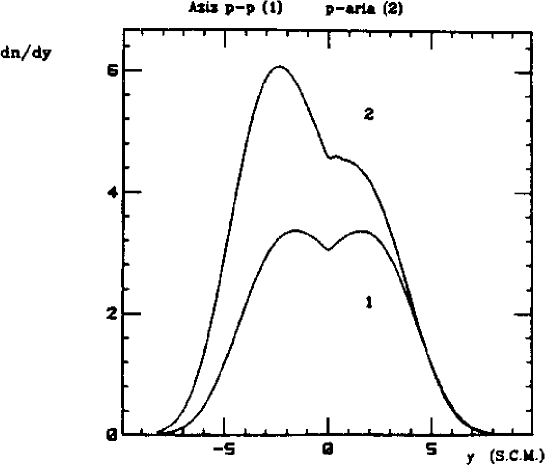
Figure 3.2: Rapidity distributions for inclusive production in $pp$ (curve 1) and $p-Air$ interactions (curve 2). In HEMAS the mean charged multiplicity for non-diffractive events is taken as twice the integral of curve 1 for $\eta>0$.

$\bullet$ Hadron $p_{t}$ in $p$-$air$ collisions is sampled using Eqs. 3.12 and 3.13 multiplied by a factor

$$R_{A,i}(p_{t})=A^{\alpha_{i}(p_{t})}$$ (3.15)

where A is the mass of the target nucleus and $i$ is the type of particle produced ($i$ = $\pi,K,p$). The factor $R_{A,i}(p_{t})$ is the ratio between the inclusive cross section on a target of mass A for the production of a particle $i$ and the corresponding cross section on a proton.

Single diffractive events
In these events, the projectile is excited to a system of mass $M$ which subsequently decays while the target nucleus remains intact. The mass $M$ of the diffractive cluster is sampled from a distribution

$$\frac{dN}{d(M^{2}/s)}=\frac{const}{M^{2}/s}$$ (3.16)

according to experimental observations at ISR [45] and $Sp\bar{p}S$ [46] at CERN. The other steps of single diffraction event modelling are similar to non-diffractive events. In this case, the decay of the diffractive cluster in the leading hadron is not isotropic as for non-diffractive events. The particle $p_{t}$ is sampled from an exponential distribution with mean value $\langle p_{t}\rangle$ = 0.45 $GeV/c$. For these events no nuclear target corrections are applied: it was checked that this approximation do not introduce relevant biases in the framework of underground muon physics.

Parametrizations
Using the HEMAS code, it is possible [31] to extract the parametrization of some parameters which are commonly used in underground muon physics, such as the muon multiplicity $N_{\mu}$ and the muon distance from the shower axis $R_{\mu}$. These parametrizations have been obtained with a set of complete Monte Carlo simulation with a primary energy ranging from 2 up to $10^{5}$ TeV and zenith angle ranging from $0^{\circ}$ e $60^{\circ}$. Only muons with energy $E_{\mu}>0.5TeV$ have been propagated in the rock. The aim of these parametrizations is to provide a fast tool when general informations are required. An accurate analysis demands the full Monte Carlo simulation chain since in these parametrizations many correlations between dynamical variables in atmosphere can be lost.

$\bullet$ The Mean number if muons produced by a primary of mass $A$, energy $E_{TOT}$, at a zenith angle $\theta$ and crossing a depth $h$ is

$$\frac{E_{\mu}<N_{\mu}>}{A\sec\theta}=f(E/E_{\mu})g(E/E_{\mu})$$ (3.17)

where

$$g(E/E_{\mu})=0.02126(E/E_{\mu})^{0.7068}(1-E_{\mu}/E)^{9.134}$$

$$f(E/E_{\mu})=\exp\left[\frac{48.27}{9.467+(E/E_{\mu})^{3.330}}\right]$$

$$E_{\mu}=0.53(e^{4\times 10^{-4}h}-1)$$

with $h$ in $hg/cm^{2}$ and $E=E_{TOT}/A$, energy per nucleon, in TeV.

$\bullet$ The multiplicity distribution $P(N_{\mu})$ is well reproduced by a negative binomial function of the form of Eq. 3.9 where the parameter $k$ is given by:

$$k=A^{2/3}10^{F(<N_{\mu}>/A)}$$

with

$${F(<N_{\mu}>/A)}=0.748+0.330\log_{10}(<N_{\mu}>/A)+0.045[\log_{10}(<N_{\mu}>/A)]^{2}$$

$\bullet$ The later distribution of muons (with respect to the shower axis) is

$$\frac{1}{N_{\mu}}\frac{dN_{\mu}}{dR_{\mu}}=\frac{(\alpha-1)(\alpha-2)}{R_{0}^{2-\alpha}}\frac{R_{\mu}}{(R_{0}+R_{\mu})^{\alpha}}$$ (3.18)

where $R_{0}$ and $\alpha$ can be expressed as a function of $<R_{\mu}>$:

$$R_{0}=\frac{\alpha-3}{2}<R_{\mu}>$$

$$\alpha=C(E)\left[\frac{1.138}{-1.126+R_{\mu}}+0.848\right]$$

where

$$C(E)=\exp(2.413-0.260X+0.0266X^{2})$$

with $X=\log_{10}[E_{TOT}(TeV)/A]$, where $E_{TOT}$ is the primary energy/nucleus.

The $<R_{\mu}>$ parameter is given by

$$<R_{\mu}>=G(E,E_{\mu},\theta)\left[11.62\,E_{\mu}^{-0.680}\left[\frac{E_{\mu}}{E}\right]^{0.114}\sec\theta\right]$$ (3.19)

where:

$$G(E,E_{\mu},\theta)=A(E,\theta)+B(E,\theta)(E_{\mu}-1)$$

$$A(E,\theta)=1.39-0.383X+6.72\times 10^{-2}X^{2}+0.1(\sec\theta-1)$$

$$B(E,\theta)=[3.14\times 10^{-2}+6.65\times 10^{-3}(X-1)](2-sec\theta)$$

HDPM

HDPM is a phenomenological generator inspired by the Dual Parton Model originally developed by Capdevielle [47] and inserted into CORSIKA as the default generator. The underlain physical picture of this generator is the formation and subsequent fragmentation of two colour strings stretched between projectile and target valence quarks. The fragmentation and hadronization processes occur around the two jets along the primary quark directions. The generator do not use any hadronization model for the production of final states particles (as the “cluster” model used in HEMAS) but simply parametrizes the particle production in each one of the two opposite jets on the basis of recent collider results. Here we do not list all the parametrized functions used in this generator; however, most of the functional forms used by HEMAS in generating the pre-particle states (the “clusters”) are here used to directly generate the finale state particles. For instance, the transverse component of the interaction is modelled according to a formula similar to Eq. 3.13, where now the $p_{t}$ is relative to the final particles and not to the clusters. The c.m. rapidities are sampled using two Gaussian distributions (for the forward and backward jets respectively) as suggested in Ref. [48]. Nuclear target effects are introduced by means the concept of intranuclear cascade, computing the actual number of “wounded” nucleons (and hence the number of elementary nucleon-nucleon collision) according to the Glauber formalism [37]. This code takes into account the so called “target excess” shown in Fig. 3.2, since it has been conceived for surface experiments where this effects can be relevant for GeV muons. This excess is parametrized into HDPM according to Ref. [48].

NIM85

This model, developed more than 15 years ago by Gaisser and Stanev [49], has been one of the first attempt to build an event generator specialized for cosmic ray physics. At present, it is well known that the model is not able to reproduce experimental data, since it introduces a non correct or too simplified treatment of hadron interactions. Nevertheless, it can be used in underground muon physics as a “trial generator” to estimate the sensitivity of a given analysis to the hadronic interaction model. The main features of this model are:
- Charged multiplicity increases as a function of the c.m. energy and the Feynman scaling violation in the central rapidity plateau is reproduced. However, the number of charged multiplicity is sampled from a Poisson distribution and not from a NBD distribution, as suggested by collider data.
- $p_{t}$ increases logarithmically as a function of the center of mass energy. However, only an exponential functional form is used in sampling the $p_{t}$, while the results of UA1 [42] show that a power law component must be included to reproduce experimental data.

This event generator has been used to extract a parametrization of the underground muon lateral distribution

$$\frac{dN_{\mu}}{dR_{\mu}}=R_{\mu}e^{-2R_{\mu}/{\langle R_{\mu}\rangle}}$$ (3.20)

with

$$R_{\mu}=A(E_{\mu})+B(E_{\mu})(E_{\mu}/E_{p})^{0.65}$$ (3.21)

where $A(E_{\mu})=4.2E_{\mu}^{-0.56}$ and $B(E_{\mu})=20.5E_{\mu}^{-0.94}$.

3.3.3 QCD inspired models

The hadronic interaction generators that we are going to present are all based on the same physical assumptions. In particular, DPMJET and SIBYLL are based on the DPM model while QGSJET is based on QGS model, two models essentially equivalent. One of the underlying common constituents of these models is the topological expansion of QCD. As suggested by t’Hooft and Veneziano, soft QCD phenomena can be quantitatively described considering a “generalized” QCD with a large number of colours $N_{c}$ and flavours $N_{f}$ such that $N_{c}/N_{f}$ = $const.$ The quantity $g^{2}_{s}N_{c}$ plays the rule of an effective running coupling constant. This trick allows to compute the diagram contribution to soft processes in the limit $N_{c}\rightarrow\infty$, and then going back to $N_{c}$ = 3 for physical applications. The interesting feature of this approach is that higher order diagrams with complicated topologies are suppressed in the cross section computation by $1/N_{c}^{2}$.

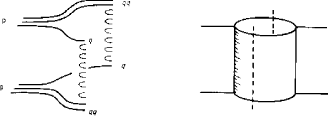
Figure 3.3: Single Pomeron exchange. The diagram has the topology of a cylinder (right) and the corresponding cutted graph, on the left, show that the dominant inelastic process is made by two string stretched between valence quark and diquark.

Each diagram involves multiple exchanges of pomerons in the $t-$channel. A Pomeron is a quasi-particle with the vacuum quantum numbers and can be seen as a mathematical realizations of the colour and gluon field stretched between the interacting partons. The dominant contribution to the elastic scattering is a single pomeron, which has the topology of a cylinder (see Fig. 3.3). The correct prescriptions for the computation of the weights of each diagrams of the topological expansion is obtained considering that there is a one-to-one correspondence between these graphs and those in Reggeon Field Theory (RFT). This theory, proposed by Gribov [50], allows to evaluate diagrams involving several reggeons and pomerons, which in this theory are quasi-particles which mediate the soft scattering phenomena. Assuming the optical model for high energy scattering, the system of two interacting hadrons can be described by the total angular momentum $l$; if we expand the scattering amplitude in partial waves

$$A(s,t)=16\pi\sum_{i=0}^{\infty}(2l+1)a_{l}(t)P_{l}(z_{t})$$ (3.22)

where $P_{l}$ are the Legendre Polynomials and $z_{t}=1+2s/(t-s_{0})$ with $s_{0}\sim 1$ GeV, it is possible to estimate the cross section of a given process summing up all the resonances in the channel $t$, i.e. considering the singularities in the complex $l$ plane (Regge poles). Each physical particle belongs to a Regge “trajectory” in the angular momentum-mass plane, of the form

$$\alpha_{k}(m_{l}^{2})=\alpha_{k}(0)+\alpha^{{}^{\prime}}_{k}(0)m_{l}^{2}=l$$ (3.23)

where the resonance masses $m_{l}$ corresponds to integer values of $l$. The pomeron corresponds to the Regge trajectory with the maximum intercept $\alpha(t=0)$. The computations of the relative contribution of each graph to the total discontinuity in the $l$ complex plane is performed by means the so called Abramovski-Gribov-Kancheli (AGK) rules. These rules provide the prescriptions to evaluate the discontinuity of a graph “cutting” the pomerons as it is shown in Fig. 3.3. The “cut” of a pomerons is a mathematical operation which consists in moving the particles on mass shell: if we associate a pomeron to a set of intermediate particle propagators (ladder) between the two external fermion lines, we can impose the momenta of the particle loop involved to be on mass shell. Each “cutted” pomeron gives rise to a pair of string stretched between valence and sea quark of the interacting particles. This operation allows to compute the discontinuity of a graph for $t$ = 0, and hence the total cross section according to the optical theorem, as shown in Fig. 3.4.

The resulting soft total cross section is of the form

$$\sigma_{soft}=g^{2}s^{\alpha(0)-1}$$ (3.24)

where $g$ is the effective nucleon-pomeron coupling constant. From the choice of the intercept $\alpha(0)$ depends the high energy regimes of the models: an intercept $\alpha(0)$ exactly equal to 1 (critical pomeron) predicts a rising cross section with the energy only due the the minijet component. On the contrary, intercepts $\alpha(0)>1$ predicts a soft component still present at high energies.

The input cross section for semi-hard production (minijets) is directly provided by the QCD improved parton model

$$\sigma_{hard}=\sum_{i,j}\int_{0}^{1}dx_{1}\int_{0}^{1}dx_{2}\int dt\frac{1}{1+\delta_{ij}}\frac{d\sigma_{QCD}^{ij}}{dt}f_{i}(x_{1},q^{2})f_{j}(x_{2},q^{2})\Theta(p_{t}-p_{t}^{thr})$$ (3.25)

where the sum runs over all the flavours and $f(x,q^{2})$ are the parton distribution functions (PDF).

The soft and hard components are different manifestation of the same process: the difference is that the hard component can be quantitatively computed by perturbative QCD. Therefore the choice of the “boundary” of the two regimes is very difficult to compute. Both the two processes (as well as the diffractive component) are treated together in these models in the framework of an Eikonal unitarization scheme. Moreover, the value of the $p_{t}^{thr}$ cut-off is chosen in such a way that at no energy and for no PDF the hard cross section is larger than the total cross section. This is to avoid unphysical rises of the minijet cross section over the total one.

The behaviour of PDFs at small values of $x$ is crucial in high energy regimes, since it determines the contrbution of the semi-hard component. After the results of the HERA experiment, we know that the singularities are of the type $1/\alpha$ with $\alpha$ between 1.35 and 1.5. At present, Monte Carlo generators uses different PDFs and this may lead to large discrepancies between the transverse structure of the final states, which are dominated by minijets at high energies.

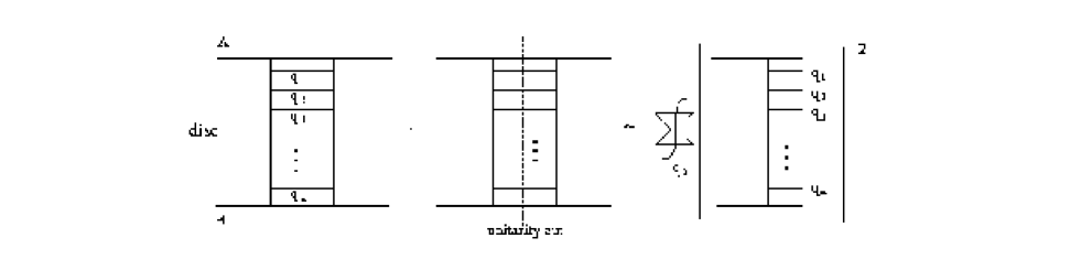
Figure 3.4: Graphical representation of the optical theorem for the one-pomeron exchange.

DPMJET

DPMJET [35] is model based on the two component DPM (the hard and soft components). Soft processes are described by a supercritical pomeron which, in the version used in this thesis (DPMJET-II.4), has an intercept $\alpha(0)$ =1.045. For hard processes hard pomerons are introduced. High mass diffractive processes are described by triple pomeron exchanges, while the low mass diffractive component is modelled outside the DPM formalism. The fragmentation of the strings, generated by the cutted pomerons, is treated using the JETSET/PYTHIA Monte Carlo routines.

DPMJET contains a detailed description of nuclear interactions (the direct interaction mentioned above). The number of nucleon-nucleon interactions is evaluated from the Glauber formalism. The intranuclear cascade of secondary particles inside the nuclei is taken into account introducing the Formation Zone Intranuclear Cascade (FZIC) concept: a naive treatment of the cascade of created secondaries inside the nucleus may lead to overestimate the overall multiplicities of created secondaries. In fact, for high energy secondaries the relativistic time dilatation inside the target nucleus may result in the generation of secondaries when they are outside the nucleus, thus not contributing to the increasing of the multiplicity.

Moreover, the model takes into account the nuclear excitation energy, which are sampled from Fermi distributions at zero temperature, nuclear fragmentation and evaporation, high energy fission and break-up of light nuclei.

DPMJET includes the production of charmed mesons, which can decay and generate prompt muons. DPMJET (from version II.3) uses the GRV-LO and CTEQ4 parton distributions; this allow the extension of the model up to energies $\sqrt{s}$ = 2000 TeV.

QGSJET

QGSJET [51] is based on the QGS model and hence has the same theoretical basis of DPMJET (Regge/Gribov theories). It uses a supercritical pomeron and the strings formed by the cutted pomerons fragment according to a procedure similar to the Lund Monte Carlo. It includes mini-jet to describe hard interactions. In nucleus-nucleus interactions the participating nucleons are determined by means the Glauber formalism and the fragmentation of the spectators are treated applying a percolation-evaporation mechanism.

SIBYLL

SIBYLL [52] is a literally minijet model, in the sense that it uses a critical pomeron with intercept $\alpha(0)$ = 1. In SIBYLL, then, all the rising cross section with energy is due to this component while the contribution of the soft component is energy independent. Soft interactions are modelled according to the picture of two colour string between a pair of quark-diquark systems. In hadron-nucleus collisions the number of interacting target nucleons $N_{W}$ determines the number of soft strings: the projectile proton is split into a quark-diquark pair which combines with one of the target wounded nucleons; the other pair of string from the remaining $N_{W}-1$ wounded nucleons combine with the sea of the projectile.

Nucleus-nucleus interactions are treated in the framework of the semi-superposition model, where the number of interacting projectile nucleons is evaluated using the Glauber formalism.

3.4 The muon transport codes

The transport of TeV muons in rock in a pre-LHC era is a difficult task since the packages used at colliders are tested for GeV muons. For instance, in [53] it is shown that GEANT 3.21 contained a not correct treatment of pair production and photo-nuclear processes; this could generate a bias in the results already at few tens of GeV. In general, muon energy loss due to ionization increases logarithmically with energy, while in the high energy tail the contribution of radiative processes (bremsstrahlung, pair production, photoproduction) is proportional to the energy

$$-\langle\frac{dE_{\mu}}{dX}\rangle=\alpha+\beta E_{\mu}$$ (3.26)

where $X$ is the rock depth, $\alpha$ is the contribution of the ionization and $\beta$ takes into account the sum of the contribution of radiative processes.

In the original transport code of HEMAS, muon transport is realized by a 3D routine which takes into account ionization energy loss, pair production, photo-production and bremsstrahlung. For each muon direction, the rock depth $X$ is computed using a detailed mountain map. The depth $X$ is then subdivided in a given number of segments $\Delta X=25\,hg/cm^{2}$, where muon energy losses are computed according to the processes quoted above. The typical energy loss in each segment $\Delta X$ is much lower than the typical muon energy ($\Delta E/E\sim 1\%$); so, during the muon transport, the angular deflection (which is dominated by Coulomb scattering) is small. Whenever the angular deflection reaches a threshold value $>1^{o}$, the step $\Delta X$ is correspondently decreased to maintain a constant accuracy in the calculation. In this code, ionization and pair production are treated as continuous processes; it was proven [53] that this approximation leads to a serious underestimation of the muon survival probability at TeV energies. In the framework of the MACRO collaboration, a dedicated code has been developed: PROPMU [54]. This package is modelled on the FLUKA code [55], but is specialized for underground experiments and it is conceived to be easily interfaced to cosmic ray generators.

3.5 Detector simulation

The detector simulator GMACRO [56] is based on the CERN package GEANT [57]. It achieves the standard tools provided by GEANT to reproduce the detector structure filling the different active volumes of MACRO with virtual materials. For instance, scintillator boxes are filled with mineral oil, streamer tube cells with gas, the iron structure of the detector with Gran Sasso rock. The positions of active volumes and read out devices are read in a data base taken from the real detector. The input event kinematic can be provided externally to GMACRO, using the full simulation chain, or can be produced with an internal generator. For each input track, GMACRO simulates all the relevant physical processes: streamer formation, pick-up signal in the strip, delta-ray production and catastrophic energy losses. Inefficiencies due to operational condition, gas mixture and electronic noise have been experimentally studied and inserted in the simulation. The number of hits due to cross talks effects correlated to the number of tracks in the event was tuned to experimental data such as the out of track hits generated by natural radioactivity.

3.6 Running the simulation

3.6.1 Choice of the composition model

Once a simulation configuration has been chosen (shower propagation code, hadronic interaction model and muon propagation in the rock) we can start the simulation chain to produce a complete MC production. The number, the mass and the energy of the primary cosmic rays to be generated have to be chosen according to a given composition model. In this work, we have used the following technique:
- each production has been performed separately for five groups of primary mass (A=1,4,14,24,56) and for each group in five contiguous energy bands. - the number of events to generate in each band has been computed according to a given composition model. Since the generation of a separate MC production for each composition model is very CPU time consuming, we have generated a single production according to a model whose flux is greater or equal to all the composition models proposed up to day. We call this model the “Overall” model and in Tab. 3.1 we report the spectrum parameters. When a given composition model is selected, each event produced with the overall model must be properly weighted

$$w(E,A)=\frac{d\phi(A)/dE}{d\phi^{*}(A)/dE}$$ (3.27)

where $d\phi^{*}(A)/dE=K^{*}E^{-\gamma^{*}}$ is the differential spectrum of the overall composition model and $d\phi(A)/dE$ is the spectrum of the chosen composition model.

Mass	$K_{1}$	$\gamma_{1}$	$E_{CUT}$	$\gamma_{2}$
Group	($m^{-2}s^{-1}sr^{-1}GeV^{\gamma_{1}-1}$)		(GeV)
P	4694.2	2.56	3.0$\times 10^{6}$	3.00
He	20494	2.74	2.0$\times 10^{6}$	3.12
CNO	600	2.50	3.0$\times 10^{6}$	3.24
Mg	400	2.50	3.0$\times 10^{6}$	3.25
Fe	310.62	2.36	2.7$\times 10^{6}$	3.00

Table 3.1: Parameters of the “overall” model.

3.6.2 Event sampling

The output of the simulation chain described consists in a sample of events at the detector level distributed over an infinite area. Each one of these events has to be properly inserted (“folded”) into the apparatus simulator in order to reproduce the detector effects. The crucial point is the choice of the shower axis position with respect to the detector position. In fact this procedure must take into account the possibility that some of the detected muons could belong to bundles with the shower axis falling outside the nominal detection area. Here we use a variance reduction method developed in [58]. We cover a fixed surface $S$ at the detector level with an array of $k=m\times n$ “pseudo-detectors” of the same dimensions of the real detector (which is placed at the center of the array). The shower axis is sampled randomly at the base area of the central detector; each one of the pseudo-detectors with at least one muon inside is considered as an individual event. The muon coordinates and director cosines of are computed in the system frame of this detector and processed separately with the detector simulator. The dimension $k$ of the array must be large enough to minimize the probability that a muon bundle with the shower axis outside the total area covered by the detector array could give a muon in the central detector. This method is extremely efficient because it excludes the possibility that a produced event could give no detectable muons. Equivalently, each produced event contributes with a factor $k$ in the computation of the live time $T$, being this event sampled independently $k$ times

$$T=\frac{kN_{prod}(\Delta E,A)}{S\Delta\Omega\Phi(\Delta E,A)}=\frac{N_{prod}(\Delta E,A)}{S_{det}\Delta\Omega\Phi(\Delta E,A)}$$ (3.28)

where $N_{prod}(\Delta E,A)$ is the number of events produced in a given band, $\Delta\Omega$ = 2.35 is the total solid angle ($\theta<60^{\circ}$), $S_{det}=S/k$ = 936 $m^{2}$ is the fiducial MACRO base area and $\Phi(\Delta E,A)$ is the integral of the energy spectrum of the chosen composition model

$$\Phi(\Delta E,A)=\int^{E_{max}}_{E_{min}}{\frac{d\phi(A)}{dE}dE}.$$ (3.29)

Chapter 4 The decoherence function

4.1 Introduction

The knowledge of hadronic interaction processes plays a fundamental role in studies of cosmic rays in the VHE–UHE range ($10^{12}$ eV $\leq E\leq 10^{17}$ eV). In particular, the interpretation of indirect measurements intended to determine the features of primary cosmic rays, such as spectra and composition, depends on the choice of the hadronic interaction model adopted in the description of the atmospheric shower development. For instance, muons observed by deep underground experiments are the decay products of mesons originating mostly in kinematic regions (high rapidity and high $\sqrt{s}$) not completely covered by existing collider data. The problem is particularly important for nucleus-nucleus interactions for which available data extend only to a few hundreds of GeV in the laboratory frame. It is therefore crucial to find physical observables which are primarily sensitive to the assumed interaction model rather than to the energy spectra and chemical composition of primary cosmic rays.

The shape of the muon lateral distribution is well-suited for this purpose. In particular it allows the study of the transverse structure of hadronic interactions, which is one of the most relevant sources of uncertainties in the models [59]. Different aspects of the interactions contribute to the lateral distribution. We can qualitatively understand this by simple arguments, valid in a first order approximation. Let us consider a single interaction of a primary nucleon of total energy $E_{0}$, producing mesons of energy $E^{\pi,K}$ with transverse momentum $P_{t}$, at a slant height $H_{prod}$, which eventually decay into muons. Calling $r$ the separation of a high energy muon (i.e. moving along a straight line) from the shower axis, we have:

$$r\sim\frac{P_{t}}{E^{\pi,K}}H_{prod}.$$ (4.1)

In this simplified description we are neglecting the transverse momentum in the parent decay. The previous expression can be written in a more instructive way, considering that at high energy, apart from terms of the order of $(m_{T}/E_{0})^{2}$, the longitudinal c.m. variable $x_{F}$ is approximately equal to the laboratory energy fraction:

$$r\sim\frac{P_{t}}{x_{F}^{\pi,K}E_{0}}H_{prod}\propto\frac{P_{t}}{x_{F}^{\pi,K}E_{0}}\left(\log{\sigma^{inel}_{n-Air}}+const.\right).$$ (4.2)

The assumption of an exponential atmosphere has been used in the last expression. It can be seen how the transverse and longitudinal components of the interaction, as well as the inclusive and total cross sections, convolve together (with different weights) to yield the lateral separation. The role of $P_{t}$ remains a dominant one in determining the relative separation of the muon component by introducing a loss of collinearity (“decoherence”) with respect to the direction of the shower axis.

A qualitative extension to the case of nuclear projectiles can be made within the framework of the superposition model, where each nucleon of the projectile of mass number A is assumed to interact independently with energy $E_{0}/A$. Further refinements are needed to account for modifications in the $P_{t}$ and $x_{F}$ distributions deriving from the nuclear structure of projectile and target, as will be discussed later. A reliable evaluation of the lateral distribution function can be obtained only by Monte Carlo methods.

Figure 4.1: Average separation of underground muon pairs at Gran Sasso depth, as a function of $\langle P_{t}\rangle$ of the parent mesons (a) and of the slant height in the atmosphere (b). The results are obtained with the HEMAS Monte Carlo.

Deep underground experiments are capable of selecting atmospheric muons in the TeV range produced in the initial stages of the extensive air shower (EAS) development. They can perform a measurement of muon separation which is highly correlated to the lateral distribution. Since the shower axis position is not usually known, the distribution of muon pair separation in multimuon events is studied. Muons associated with the same events, coming in general from different parent and shower generations, are grouped together. Furthermore, a wide range of primary energy is integrated in the same distribution. It is generally assumed, and supported by many simulations, that the shape of this distribution is only slightly affected by the mass composition of primaries [60], thus preserving the sensitivity to the interaction features. As an example, in Fig. 4.1 we show the dependence of the average pair separation, as detected at the depth of the underground Gran Sasso laboratory, with respect to the $\langle P_{t}\rangle$ of the parent mesons and to their production slant height in the atmosphere. These have been calculated by means of the HEMAS Monte Carlo code [31] for a mixed primary composition [16]. This code employs an interaction model based on the results of the experiments at hadron colliders.

The decoherence function as measured in an underground experiment is also affected by multiple scattering in the rock and, to some extent, geomagnetic deflection.

For a detector with geometrical acceptance $A(\theta,\phi)$, for zenith and azimuthal angles $\theta$ and $\phi$, respectively, we define the decoherence function as the distribution of the distance between muon pairs in a bundle:

$$\frac{dN}{dD}=\frac{1}{\Omega T}\int{\frac{1}{A(\theta,\phi)}\frac{d^{2}N(D,\theta,\phi)}{dDd\Omega}d\Omega},$$ (4.3)

where $N(D,\theta,\phi)$ is the number of muon pairs with a separation $D$ in the direction ($\theta$,$\phi$), $\Omega$ is the total solid angle covered by the apparatus and $T$ is the total exposure time of the experiment. A muon bundle event of multiplicity $N_{\mu}$ will contribute with a number of independent pairs $N=N_{\mu}(N_{\mu}-1)/2$.

In principle, a decoherence study can be performed without a single large area detector, and in early attempts the muon lateral separation was studied via coincidences between two separate movable detectors [61]. The advantage offered by a single large area detector is the ability to study the features inherent in the same multi-muon event, such as higher order moments of the decoherence distribution (see next Chapter).

An analysis of the muon decoherence has already been performed [62, 63, 15, 16]. The bulk of multiple muon events in MACRO corresponds to a selection of primary energies between a few tens to a few thousands of TeV/nucleon. Hadronic interactions and shower development in the atmosphere were simulated with the HEMAS code. In particular, a weak dependence on primary mass composition was confirmed for two extreme cases: the “heavy” and “light” composition models presented in Chapt 1. The MACRO analysis was designed to unfold the true muon decoherence function from the measured one by properly considering the geometrical containment and track resolution efficiencies. This procedure allows a direct comparison between measurements performed by different detectors at the same depth, and, more importantly, whenever new Monte Carlo simulations are available, allows a fast comparison between predictions and data without the need to reproduce all the details of the detector response.

The first attempt, obtained while the detector was still under construction, and therefore with a limited size, was presented in [62]. The same analysis, with a larger sample based on the full lower detector, was extended in [63]. With respect to the HEMAS Monte Carlo expectations, these results indicated a possible excess in the observed distribution at large separations. In Ref. [16] we presented the decoherence distribution without the unfolding procedure; the claimed excesses were not confirmed. In order to reach more definitive conclusions, a more careful analysis of the systematics associated with the unfolding procedure was considered necessary. A detailed discussion of this item will be addressed in Section 4.7.

A more careful discussion of the Monte Carlo simulation is also necessary. The bulk of the muon bundles collected by MACRO are low multiplicity events, coming from parent mesons in the far forward region of UHE interactions, not easily accessible with collider experiments. This requires an extrapolation to the highest energies and rapidity regions, introducing possible systematic uncertainties. For instance, some doubts have been raised [59] concerning the treatment of meson $P_{t}$ in HEMAS. In the HEMAS hadronic interaction code, secondary particle $P_{t}$ depends upon three different contributions:

• $\langle P_{t}\rangle$ increases with energy, as required by collider data in the central region;

• $\langle P_{t}\rangle$ increases in p–Nucleus and Nucleus–Nucleus interactions, relative to that for pp collisions, according to the “Cronin effect” [64];

• $\langle P_{t}\rangle$ varies with $x_{F}$, according to the so called “seagull effect” [65].

The sum of these effects yields some doubts about a possible overestimate of $P_{t}$ for energetic secondary particles, an hypothesis recently restated in [66]. It is therefore crucial to perform a high precision test of the transverse structure of this model, since it affects the calculation of containment probability for multiple muon events and, consequently, the analysis of primary cosmic ray composition [15, 16].

In this work, a new analysis of the unfolded decoherence function is presented, performed with improved methods up to 70 m. The present work enlarges and completes the data analysis presented in [15, 16]. Preliminary results of this unfolding procedure [67] showed an improved agreement between experimental data and Monte Carlo predictions.

Particular attention is paid to the small-separation ($D\leq 1$ m) region of the decoherence curve, in which processes such as muon-induced hadron production can produce a background to the high energy muon analysis. At the energies involved in the present analysis ($E_{\mu}\geq$ 1 TeV), moreover, muon-induced muon pair production in the rock overburden could yield an excess of events with small separation, as suggested in [68]. This process is usually neglected in Monte Carlo models commonly adopted for high energy muon transport [31, 55, 57, 54].

4.2 Event selection and data analysis

In reconstructing the best bundle configuration, the tracking package flags track pairs as parallel, overlapping, or independent and not parallel. This is achieved in two steps, in each projective view:

• two tracks are defined as parallel if their slopes coincide within 2 $\sigma$ or if their angular separation is less than $3^{0}$ ($6^{0}$ if the tracks contain clusters whose widths exceed 30 cm). Otherwise, the track pair is flagged as independent and not parallel if its distance separation is larger than 100 cm.

• tracks at short relative distance are labelled as overlapping if their intercepts with the detector bottom level coincide within 3.2 $\sigma$ (2 $\sigma$ if their angular separation is $<1.5^{0}$).

The routine chooses the most likely bundle as the set having the largest number of parallel tracks and the largest number of points per track. Subsequently, tracks flagged as not parallel are considered in order to include fake muon tracks originated primarily by hadrons or $\delta$-rays in the surrounding rock or inside the detector. A two-track separation of the order of 5 cm is achieved on each projective view. However, this capability can be substantially worsened in case of very large, but rare, catastrophic energy losses of muons in the detector.

Only tracks with a unique association in the two views can be reconstructed in three dimensions. At this level, pattern recognition is used to require a complete matching between tracks belonging to different projective views. This is automatically achieved when two tracks pass through separate detector modules. When they are in the same module, matching of hit wires and strips on the same detector plane is accomplished by taking advantage of the stereo angle of the strips with respect to the wires. In some cases the track pattern correspondence between the two views is also used. The possibility to analyse muon decoherence in three dimensional space is important to have an unbiased decoherence distribution. However, the unambiguous association of muon tracks from the two projective views cannot be accomplished for high multiplicity events because, in events characterized by a high muon density, the tracking algorithm is not able to resolve the real muon pattern without ambiguities, especially when tracks are superimposed. In Ref. [15, 16] we presented the muon decoherence function in the wire view alone, which allowed the extension of the analysis to higher multiplicities.

We have analyzed about $3.4\cdot 10^{5}$ multi muon events, corresponding to a 7732 hr live time for the lower part of the apparatus. These events were submitted to the following selection criteria:

1. Zenith angle smaller than $60^{0}$. This choice is dictated by our limited knowledge of the Gran Sasso topographical map for high zenith angles. Moreover, we cannot disregard the atmosphere’s curvature for larger zenith angles, which at present our current simulation models do not include.

2. Fewer than 45 streamer tube hits out of track. This selection is designed to eliminate possible misleading track reconstruction in events produced by noise in the streamer tube system and/or electromagnetic interactions in or near the apparatus.

3. Track pairs must survive the parallelism cut. This rejects hadrons from photonuclear interactions close to the detector, as well as tracks reconstructed from electromagnetic interactions which survived the previous cut.

The last cut is not completely efficient in rejecting muon tracks originating from local particle production because the angle between these tracks may fall within the limits imposed by the parallelism cut. These limits cannot be further reduced since the average angular divergence due to multiple muon scattering in the rock overburden is about $1^{0}$ at the MACRO depth. This is a crucial point, since these events could contaminate the decoherence curve in the low separation region and are not present in the simulated data because of the excessive CPU time required to follow individual secondary particles. A similar effect could be produced by single muon tracks with large clusters, which may be reconstructed as a di-muon event by the tracking algorithm.

In order to reduce these effects, a further selection was applied. We computed, for each muon track in the wire view, the ratio $R$ between the number of streamer tube planes hit by the muon to the number of planes expected to be hit considering the track direction. Only tracks with $R\geq 0.75$ were accepted. The application of this cut (hereafter cut C4) in the wire view alone is a good compromise between the rejection capability of the algorithm and the loss of events due to the unavoidable inefficiency of the streamer tube system. We found that in the wire projective view the probability to reject a muon track due to contiguous, inefficient planes is 2.0%.

Figure 4.2: The change in the experimental decoherence function induced by cut C4. The data indicate the fractional deviation between the experimental decoherence function before and after the application of the cut.

To show the effects produced by cut C4, we present in Fig. 4.2 the fractional differences between the experimental decoherence curve before and after its application. As expected, the new cut affects only the first bins of the distribution.

Figure 4.3: Percentage of reconstructed real events (white points) and unambiguously associated muon pairs (black points) as a function of event multiplicity.

To test the ability of cut C4 to reject hadronic tracks, we used FLUKA [55] to simulate 3028 hr of live time in which muons were accompanied by hadronic products of photonuclear interactions in the 10 m of rock surrounding the detector. We found that the parallelism cut alone provides a rejection efficiency of about 54.6% of the pair sample, while the addition of cut C4 enhances the rejection to 95.9%. The effect of hadron contamination, furthermore, is very small, contributing less than 1% in the overall muon pair sample. This estimate, together with the plot of Fig. 4.2 and the results of a visual scan, suggest that the main track sample rejected by cut C4 is made of large cluster tracks. After the overall application of these cuts, the number of surviving unambiguously associated muon pair tracks is 355,795. In Fig. 4.3 the percentage of the reconstructed events as a function of muon multiplicity is shown (open circles). In the same figure, the percentage of the unambiguously associated muon pairs as a function of the multiplicity is also reported (black circles). Due to detector effects, the number of associated pairs $N^{\prime}_{pair}$ in an event of multiplicity $N_{\mu}$ is generally smaller than the maximum number of independent pairs $N_{pair}=N_{\mu}(N_{\mu}-1)/2$. This reduction becomes greater for high multiplicities, for obvious reasons of track shadowing. In any case, we still find that the weight of high multiplicity events remains dominant in the decoherence distribution. In order to reduce this effect and to reduce the possible dependence on primary composition, we have assigned a weight $1/N^{\prime}_{pair}$ to each entry of the separation distribution. This prescription, followed also for simulated data, has been already applied in most of the previous analyses performed by MACRO. Moreover, we emphasize that the focus of this analysis is centered on the shape of the distribution; the absolute rate of pairs as a function of their separation is neglected.

4.3 Monte Carlo Simulation

We have used, as in all previous relevant analyses of muon events in MACRO [15, 16], the HEMAS code [31] as an interaction model and shower simulator. Nuclear projectiles are handled by interfacing HEMAS with the “semi-superposition” model of the NUCLIB library [36]. The final relevant piece of simulation is the three-dimensional description of muon transport in the rock.

In order to verify possible systematics affecting the decoherence distribution connected with the muon transport code in the rock, we performed two Monte Carlo productions using two different transport codes. The first production has been realized with the transport code included in the original HEMAS version [31] and the second production with the PROPMU code [54]. We have verified that, at least to first approximation, no changes in the shape of the decoherence function are noticeable between the two different simulation samples. For this reason, the sum of the two different Monte Carlo productions will be used in the following.

In Tab. 4.1 is reported the number of events generated according to the “overall” model for each of the five mass groups considered. Being the generation of the first energy bands very CPU time consuming, we have generated a reduced statistics for low energy events: for the first (second) MC production, only 1/5 of the events with energy $E_{primary}<2000$ TeV ($E_{primary}<20$ TeV) have been generated. The low energy events have been properly weighted when included in the analysis.

Primary	Primary	Number of events	Fraction of	Fraction of
Type	Energy (TeV)	to simulate	simulated evt	simulated evts
		(Overall Model)	(I production)	(II production)
	3–20	8.99E+8	1/5	1/10
	20–200	4.78E+7	1/5	1/2
P	200–2000	1.3E+6	1/5	1/2
	2000–20000	32616	1	1/2
	20000–100000	334	1	1/2
	12–20	4.685+07	1/5	1/10
	20–200	3.212E+07	1/5	1/2
He	200–2000	584366	1/5	1/2
	2000–20000	8822	1	1/2
	20000–100000	65	1	1/2
	20–200	1.15E+7	1/5	1/2
CNO	200–2000	366378	1/5	1/2
	2000–100000	9750	1	1/2
	20000–100000	61	1	1/2
	20–200	7.72E+6	1/5	1/2
Mg	200–2000	244248	1/5	1/2
	2000–20000	6488	1	1/2
	20000–100000	39	1	1/2
	20–200	2.61E+7	1/5	1/2
Fe	200–2000	1.14E+6	1/5	1/2
	2000-20000	40570	1	1/2
	20000–100000	412	1	1/2

Table 4.1: Statistical sample of the two MC productions used in the decoherence analysis. In correspondence of each energy band, it is shown the number of events to generate according to the “overall” model. The last two columns report the effective fractions of events produced.

The map of Gran Sasso overburden as a function of direction and the description of its chemical composition are reported in Ref. [69].

The folding of simulated events with the detector simulation is performed according to the variance reduction method explained in the previous Section. In the first (second) production of Tab. 4.1 we used an array of 7$\times$3 (13$\times$5) detectors corresponding to an area of $231.\times 88.2\,m^{2}$ ($380.3.\times 153.4\,m^{2}$). We assumed the “MACRO-fit” primary mass composition model and each event has been weighted according to Eq. 3.27.

Simulated data are produced with the same format as real data and are processed using the same analysis tools. After the application of the same cuts as for real data, a sample of about $7.0\cdot 10^{5}$ muon pairs survived, corresponding to about 645 days of MACRO live time.

4.4 Comparison of experimental and Monte Carlo data

Figure 4.4: Experimental (black points) and simulated (white points) decoherence function, normalized to the peak of the $dN/dD$ distribution. The second to the last points of the two distributions coincide.

In Fig. 4.4 the comparison between the experimental and simulated decoherence curve inside the detector is shown. Curves are normalized to the peak of the $dN/dD$ distribution. The remarkable consistency of the two curves demonstrates the HEMAS code capability to reproduce the observed data up to a maximum distance of 70 m. The bump in the experimental distribution around 40 m is due to the detector acceptance and is visible also in the simulated data, thus confirming the accuracy of our detector simulation. We also notice that, despite the application of cut C4, there is a non-negligible discrepancy between the experimental and simulated data in the first two bins of the distribution of ($34\pm 2$)% and ($10\pm 1$)%, respectively. Such a discrepancy is not predicted by any model, since at short distances, apart from detector effects, the shape of decoherence distribution is dictated by the solid angle scaling: $dN/dD^{2}|_{D\rightarrow 0}\sim const.$, while the relevant properties of the interactions under investigation manifest themselves in the shape at large distances. The origin of this discrepancy will be discussed in detail in Section 4.7, where other sources of contamination in the real data sample will be taken into account.

4.5 Unfolding Procedure

The agreement of the Monte Carlo and data shown in Fig. 4.4 proves that the simulation is consistent with observation and that the detector structure is well reproduced. A detector-independent analysis is required in order to subtract the geometric effects peculiar to MACRO; furthermore it allows a more direct comparison with other analyses and/or hadronic interaction models. This is accomplished by a correction method, built with the help of the Monte Carlo simulation, to unfold the “true” decoherence function from the measured one in which geometrical containment and track reconstruction efficiencies are considered.

Figure 4.5: Comparison of the unfolding efficiencies as a function of pair separation for different composition models. The curves are normalized to the peak value. For comparison, we include the efficiency evaluated with the method used in previous analyses (open circles).

In the previous decoherence studies [62, 63], the unfolding procedure was based on the evaluation of the detection efficiency for di-muon events generated by the Monte Carlo with a given angle and separation. Although this method is composition independent and allowed us to determine the detector acceptance with high statistical accuracy, it introduces systematic effects that have so far been neglected. In particular, in a multi-muon event it may happen that in a given projective view and in a particular geometrical configuration one muon track is “shadowed” by another. To avoid this effect, we adopt the following new unfolding method: the efficiency evaluation is performed considering the whole sample of events generated with their multiplicities. For a given bin of ($D$,$\theta$,$\phi$), where $D$ is the muon pair separation and ($\theta$,$\phi$) is the arrival direction of the event, we calculate the ratio

$$\epsilon(D,\theta,\phi)=\frac{N^{in}(D,\theta,\phi)}{N^{out}(D,\theta,\phi)}$$ (4.4)

between the number of pairs surviving the selection cuts $N^{in}$ and the number of pairs inserted in the detector simulator $N^{out}$. In principle, this choice of $\epsilon$ could be dependent on the primary mass composition model, since for a fixed distance $D$ the efficiency (Eq. 4.4) is dependent on the muon density and hence on its multiplicity, which in turn is correlated with the average atomic mass $\langle A\rangle$ of the primary. To check the systematic uncertainty related to this possibility, we evaluated the decoherence distributions obtained by unfolding the experimental data assuming the “heavy” and “light” composition models. Fig. 4.5 shows the relative comparison of the shape of the unfolding efficiencies as a function of pair separation, integrated in $(cos\theta,\phi)$ after the normalization to the peak value. In the same plot we present the unfolding efficiency calculated with the method used in Ref. [62, 63]. Considering the effect of the normalization, we observe that this method tends to overestimate the efficiencies in the low distance range, a consequence of the shadowing effect as explained in Section 4.2.

The unfolded decoherence is given by

$$\left(\frac{dN}{dD}\right)_{unf}=\sum_{(\theta,\phi)}\frac{N^{exp}(D,\theta,\phi)}{\epsilon(D,\theta,\phi)},$$ (4.5)

where $N^{exp}(D,\theta,\phi)$ is the number of muon pairs detected with a separation $D$. In practice, we used 50 windows in $(cos\theta,\phi)$ space (5 and 10 equal intervals for $\cos\theta$ and $\phi$, respectively).

The ability to evaluate the integral 4.5 to separate and independent windows is a powerful check of the systematics related to the decoherence dependence on the variables $(cos\theta,\phi)$. Unfortunately this is not possible for $r$ larger than 45 m, due to insufficient statistics. In that case the observables $N^{in},N^{out}$ and $N^{exp}$ are integrated over $(cos\theta,\phi)$. We verified that the systematic error introduced by that choice is smaller than the present statistical error in that distance range.

Figure 4.6: Unfolded experimental decoherence distribution compared with the infinite-detector Monte Carlo expectation, computed with the HEMAS interaction code and the MACRO-fit primary composition model. Black squares represent data above 45 m (integral form unfolding).

Finally, unfolded experimental data obtained with the MACRO-fit model are directly compared with the Monte Carlo simulation (Fig. 4.6). The two curves are in good agreement although the disparity in the first bin of the distribution remains unresolved (see Section 4.7). The experimental values of the $dN/dD$ distributions, normalized to the peak value, are reported in Table 4.2.

D (cm)	$dN/dD$	Error
80	0.425	0.010
240	0.885	0.016
400	1.000	0.017
560	0.959	0.017
720	0.815	0.015
880	0.673	0.014
1040	0.559	0.013
1200	0.434	0.012
1360	0.341	0.011
1520	0.294	0.011
1680	0.2198	0.0049
1840	0.1828	0.0046
2000	0.1578	0.0045
2160	0.1283	0.0041
2320	0.1047	0.0039
2480	0.0935	0.0039
2640	0.0744	0.0036
2800	0.0585	0.0032
2960	0.0517	0.0032
3120	0.0417	0.0030
3280	0.0411	0.0031
3440	0.0258	0.0026
3600	0.0231	0.0024
3760	0.0226	0.0025
3920	0.0200	0.0025
4080	0.0129	0.0020
4240	0.0142	0.0023
4400	0.0091	0.0018
4560	0.0068	0.0016
4720	0.0031	0.0010
4880	0.0030	0.0011
4640	0.0113	0.0033
4960	0.0087	0.0045
5280	0.0071	0.0041
5600	0.0037	0.0015
5920	0.0042	0.0027
6240	0.0030	0.0027
6560	0.00075	0.00090

Table 4.2: Tabulation of the the unfolded decoherence distribution as measured by MACRO. The data points are normalized to the point of maximum.

4.6 Uncertainties of the hadronic interaction model

The present work, as others from MACRO, is extensively based on the HEMAS code. This was explicitly designed to provide a fast tool for production of high energy muons ($E_{\mu}>$500 GeV). However, as mentioned before, the interaction model of HEMAS is based on parametrizations of existing accelerator data and therefore is subject to the same risks of all this class of simulation codes. In particular, important correlations might be lost, or wrong, or the necessary extrapolations required by the specific kinematic regions of cosmic ray physics could yield unrealistic results.

In the previous Chapter we have introduced some of the “physically inspired” codes commonly used in CR physics at present. A review of general results obtained using CORSIKA with those models has been provided by the Karlsruhe group [70]. A common feature of all these models is the more or less direct reference to the Regge-Gribov theories [50] for the soft contribution (low $P_{t}$). It must be stressed that such a phenomenological framework, by its nature, provides only predictions for the longitudinal properties of the interaction. The transverse structure leading to the specific $P_{t}$ distribution is not constrained by the theory, except for the higher $P_{t}$ phenomena, where perturbative QCD can be used (this is of small relevance in the primary energy region addressed by the MACRO data). Once again, the model builders have to be guided mostly by experimental data, introducing a-priori functional forms along with their additional required parameters. Some of the quoted models introduce proper recipes for the continuity between the soft and perturbative QCD regimes, and also specific nuclear phenomena like the Cronin effect mentioned above (see for instance [35]). In practice, the only possibility to evaluate a systematic uncertainty associated with the simulation model (at least those concerning the transverse structure of the showers) is to compare the predictions from all these models, HEMAS included. For this purpose, since the Karlsruhe report [70] did not address this point, we have performed test runs with some of the models interfaced to CORSIKA, to which PROPMU [54] has also been interfaced by us for muon transport in the rock overburden. A full simulation with all the other codes was outside our present capability, so we limited ourselves to comparisons at a few fixed primary energies, and at fixed primary angles of 30^∘ in zenith and 190^∘ in azimuth. These correspond to an average rock overburden of $\sim$ 3200 hg/cm².

p–Air, 20 TeV Code $\langle X_{first}\rangle$ $\langle P_{t}\rangle$ $\pi^{\pm}$ $\langle H_{\mu}\rangle$ $\langle R\rangle$ $\langle D\rangle$ (g/cm²) (GeV/c) (km) (m) (m) HEMAS 51.4 0.40 24.1 7.9 12.7 CORSIKA/DPMJET 44.4 0.42 25.6 10.1 13.9 CORSIKA/QGSJET 45.7 0.39 24.3 7.3 10.0 CORSIKA/VENUS 48.3 0.35 24.5 7.4 8.3 CORSIKA/SIBYLL 50.9 0.37 23.5 7.2 11.5
p–Air, 200 TeV Code $\langle X_{first}\rangle$ $\langle P_{t}\rangle$ $\pi^{\pm}$ $\langle H_{\mu}\rangle$ $\langle R\rangle$ $\langle D\rangle$ (g/cm²) (GeV/c) (km) (m) (m) HEMAS 56.1 0.44 20.6 5.3 8.0 CORSIKA/DPMJET 53.9 0.43 21.7 6.2 8.8 CORSIKA/QGSJET 52.8 0.41 21.4 5.5 7.8 CORSIKA/VENUS 60.2 0.36 20.9 5.3 7.5 CORSIKA/SIBYLL 55.2 0.41 20.2 5.2 7.3
p–Air, 2000 TeV Code $\langle X_{first}\rangle$ $\langle P_{t}\rangle$ $\pi^{\pm}$ $\langle H_{\mu}\rangle$ $\langle R\rangle$ $\langle D\rangle$ (g/cm²) (GeV/c) (km) (m) (m) HEMAS 63.0 0.50 16.3 4.1 6.0 CORSIKA/DPMJET 60.0 0.42 18.5 4.9 6.4 CORSIKA/QGSJET 63.1 0.44 17.7 4.2 5.6 CORSIKA/VENUS 66.7 0.36 16.8 4.1 5.3 CORSIKA/SIBYLL 60.3 0.44 17.0 4.4 5.6

Table 4.3: Comparison of a few simulated relevant quantities concerning the lateral distribution of underground muons at the depth of 3200 hg/cm², from proton primaries at 20, 200 and 2000 TeV, 30^∘ zenith angle. The statistical errors are smaller than the last reported digit.

In Tables 4.3 we show this comparison for a few representative average quantities for 3 different primary proton energies. We have considered the average depth of the first interaction $X$, $\langle P_{t}\rangle$ for pions coming from the first interaction, the average production slant height $H_{\mu}$ of muons surviving underground (the decay height of their parent mesons.), the average distance of the muons from shower axis $\langle R\rangle$ and the average underground decoherence $\langle D\rangle$. Before discussing the results, it is important to remark that as far single interactions are concerned, all the models considered give a $P_{t}$ distribution following, with good approximation, the typical power law suggested by accelerator data. This is $\propto 1/(P_{t}+P_{0})^{\alpha}$, although with somewhat different parameters for different models. Older models, like those predicting a simple exponential distribution for $P_{t}$, cannot reproduce the muon lateral distribution observed in MACRO data [62].

Figure 4.7: Unfolded decoherence functions compared with Monte Carlo simulations for different $cos\theta$ windows. The vertical scale is in arbitrary units.

In the energy range of 100-1000 TeV, to which most of MACRO data belong, the resulting differences in the average muon separation do not exceed 20%. These discrepancies seem to become smaller at higher energy, while they appear to be much larger at few tens of TeV. DPMJET is probably the only model predicting a higher average separation than HEMAS. A precise analysis of the reasons leading to the differences among models is complicated. However, we note that HEMAS gives, in general, higher values of the average $P_{t}$ than the other models. The only exception is indeed DPMJET, which, as mentioned before, pays particular attention to the reproduction of nuclear effects affecting the transverse momentum, as measured in heavy ion experiments [71]. On the other hand, the effect of this large $P_{t}$ on the lateral distribution of muons is moderated in HEMAS by a deeper shower penetration (the inelastic cross section is based on Ref. [72]); in general HEMAS exhibits a somewhat smaller height of meson production.

Similar features in the comparison of models are also obtained for nuclear projectiles. It is therefore conceivable that, for the same primary spectrum and composition, not all the models considered could reproduce the MACRO decoherence curve. Thus the best fit for spectrum and composition as derived from the analysis of muon multiplicity distribution in MACRO will also probably differ according to the model.

At least in part, the decoherence analysis can disentangle different ranges of longitudinal components of the interaction from the transverse ones, if this is performed in different zenith angle and rock depth windows. In fact, larger zenith angles correspond (on average) to larger muon production slant heights. This is a geometrical effect due to the greater distance from the primary interaction point to the detector for large zenith angle and consequently to the greater spreading of the muon bundle before reaching the apparatus. Larger rock depths select higher energy muons and consequently higher average energy of their parent mesons. The average separation decreases with the rock depth since, qualitatively, the longitudinal momentum $\langle P_{\parallel}\rangle$ increases linearly with energy while $\langle P_{t}\rangle$ increases only logarithmically. The overall result of increasing rock depth is the production of final states in a narrower forward cone, decreasing the muon pair average separation observed at the detector level.

Figure 4.8: Unfolded decoherence functions compared with Monte Carlo simulations for different rock depth windows.

In Fig. 4.7 and 4.8 the unfolded decoherence function is compared to the HEMAS prediction for different zenith and rock depth intervals. In Table 4.4, the average separation $\langle D\rangle$ is reported as a function of $cos\theta$ and rock depth for fixed rock depth and zenith, respectively. In the same table we report the average values of slant height of first interaction $\langle X\rangle$, muon production slant height $\langle H_{\mu}\rangle$, energy $\langle E_{p}\rangle$ and transverse momentum $\langle P_{t}\rangle$ of the parent mesons, as obtained from the HEMAS Monte Carlo in the same windows.

3750$<$h$<$4150 ($hg/cm^{2}$) .5$<$cos$\theta$$<$.6 .6$<$cos$\theta$$<$.7 .7$<$cos$\theta$$<$.8 .8$<$cos$\theta$$<$.9 .9$<$cos$\theta$$<$1. EXP $\langle D\rangle$ (m) $13.2\pm 2.3$ $11.4\pm 2.2$ $10.3\pm 2.2$ $8.5\pm 1.9$ $7.5\pm 1.9$ $\langle D\rangle$ (m) $12.8\pm 1.4$ $12.0\pm 1.3$ $10.1\pm 1.2$ $8.8\pm 1.2$ $7.8\pm 1.1$ $\langle X\rangle$ (km) $65.9\pm 0.2$ $57.0\pm 0.2$ $51.2\pm 0.3$ $42.5\pm 0.4$ $37.0\pm 0.5$ MC $\langle H_{\mu}\rangle$ (km) $41.6\pm 0.3$ $34.3\pm 0.3$ $28.1\pm 0.3$ $23.8\pm 0.3$ $20.4\pm 0.3$ $\langle E_{p}\rangle$ (TeV) $4.1\pm 0.2$ $4.0\pm 0.2$ $4.0\pm 02$ $3.9\pm 0.1$ $3.9\pm 0.2$ $\langle P_{t}\rangle$ (GeV/c) $0.56\pm 0.01$ $0.59\pm 0.01$ $0.57\pm 0.01$ $0.57\pm 0.02$ $0.57\pm 0.01$ (a)

0.8$<$cos$\theta$$<$0.9 3350$<$h$<$3750 3750$<$h$<$4150 4150$<$h$<$4550 4550$<$h$<$4950 ($hg/cm^{2}$) ($hg/cm^{2}$) ($hg/cm^{2}$) ($hg/cm^{2}$) EXP $\langle D\rangle$ (m) $9.4\pm 2.1$ $8.5\pm 1.9$ $7.3\pm 1.6$ $6.2\pm 1.6$ $\langle D\rangle$ (m) $9.7\pm 3.4$ $8.8\pm 1.2$ $7.7\pm 1.1$ $7.1\pm 1.1$ $\langle X\rangle$ (km) $42.7\pm 0.4$ $42.5\pm.4$ $45.9\pm 0.3$ $43.76\pm 0.3$ MC $\langle H_{\mu}\rangle$ (km) $23.7\pm 0.3$ $23.8\pm 0.3$ $24.6\pm 0.3$ $25.1\pm 0.5$ $\langle E_{p}\rangle$ (TeV) $3.6\pm 0.1$ $3.9\pm 0.1$ $4.4\pm 0.1$ $4.8\pm 0.02$ $\langle P_{t}\rangle$ (GeV/c) $0.56\pm 0.02$ $0.57\pm 0.02$ $0.58\pm 0.02$ $0.58\pm 0.02$ (b)

Table 4.4: Average separation between muon pairs $\langle D\rangle$ (in m) as a function of cos$\theta$ (a) and rock depth (b). In each table the experimental data are compared to the expectations from the HEMAS Monte Carlo. For the same simulations, the averages of other quantities are reported.

The agreement between the results and the Monte Carlo in separate variable intervals reinforces our confidence in the capability of HEMAS to reproduce the significant features of shower development. This also allows us to exclude the existence of significant systematic errors related to this analysis.

4.7 The contribution of the $\mu^{\pm}+N\rightarrow\mu^{\pm}+N+\mu^{+}+\mu^{-}$ process

The capability of the MACRO detector to resolve very closely spaced tracks allows the extension of the decoherence analysis to a distance region hardly studied in the past. The mismatch between experimental and simulated data in this region ($D\leq$ 160 cm) has been emphasized earlier in our discussion. In Section 4.2 a solution was attempted, permitting us to discard, with high efficiency, those tracks originating from secondary particle production. However, Fig. 4.4 and Fig. 4.6 show that other sources of contamination in the first bin of the decoherence function are responsible for the discrepancy.

The process of muon pair production by muons in the rock, $\mu^{\pm}+N\rightarrow\mu^{\pm}+N+\mu^{+}+\mu^{-}$, is a natural candidate. As pointed out in [68], at the typical muon energies involved in underground analyses ($E_{\mu}\sim$ 1 TeV) and for very large energy transfer, the cross section for this process is non-negligible with respect to e⁺e^- pair production. An analytic expression for the muon pair production cross section is given in [68, 73]. In order to test the hypothesis, this cross section has been included in the muon transport code PROPMU. Assuming a muon flux with energy spectrum $E^{-3.7}$ and minimum muon energy $E_{\mu}^{min}$ = 1.2 TeV at the surface, and considering the actual mountain profile, we generated a sample of $10^{7}$ muons corresponding to 3666 h of live time. About $\sim 3.0\cdot 10^{6}$ muons survived to the MACRO level, 5360 of which were generated by muon pair production processes. The average separation of these muon pairs is $(128\pm 1)$ cm, and their average residual energies are $(657\pm 14)$ GeV and $(145\pm 3)$ GeV, respectively, for the main muon and the secondary muon samples. We propagated the muons surviving to the MACRO level through the GEANT simulation and we applied the same cuts specified in Section 4.2. Finally, the number of events was normalized to the live time of real data.

	0–80 cm	80–160 cm	160–240 cm	240–320 cm	320–400 cm
					(max)
Exp. Data	5528	12491	17569	20514	20816
MC Data	5154	21417	33573	40367	42679
Discrepancy after	(55$\pm$2)%	(16$\pm$2)%	(6$\pm$1)%	(4$\pm$1)%
normalization
Exp. Data + C4	3612	11128	16535	19597	19977
MC Data + C4	4848	20346	31932	38425	40660
Discrepancy after	(34$\pm$2)%	(10$\pm$2)%	(6$\pm$2)%	(4$\pm$2)%
normalization
Exp. Data + C4 +	2193	9264	15462	19190	19842
$\mu$ pair subtraction
MC Data + C4	4848	20346	31932	38425	40660
Discrepancy after	(8$\pm$7)%	(7$\pm$3)%	(0$\pm$2)%	(2$\pm$2)%
normalization

Table 4.5: Number of weighted muon pairs in the first few bins of the experimental and simulated decoherence distributions. The discrepancy is the percentage difference between experimental and Monte Carlo values, normalized to the distribution maximum (last column).

In Table 4.5 we report the number of weighted muon pairs in the first bins of the experimental and simulated decoherence distributions (in the form $dN/dD$). The effect of standard cuts, of cut C4, and of the subtraction of the muon pair production process are shown in order. In each case, we indicated in percentage the bin populations with respect to the peak of the distribution and the discrepancy with respect to the Monte Carlo predictions.

Figure 4.9: The low distance region of the experimental decoherence function, before and after the subtraction of the secondary muon sample, and comparison with the Monte Carlo simulation. The inset shows the distribution of relative distances for muon pairs in excess of the data after the subtraction of the HEMAS prediction, compared to the expectation from simulated muon pair production in the rock.

In Fig. 4.9 we compare the simulated decoherence curve with the data corrected for the muon pair production effect. Despite the approximation introduced in our test, it seems that the proposed muon pair production process can account for most of the observed discrepancy in the low distance range. This is also shown in the inset of Fig. 4.9 where the distribution of relative distance for the muon pairs in excess of the data (after subtraction of HEMAS prediction) is compared to the expectation from simulated muon pair production.

Recently, after the publication of the present work in [74], a new calculation of the muon pair production cross section appeared in [75] together with an estimation of double and triple muon event rates due to this process. In that work, the approximation of a point-like scattering nucleus was abandoned and nuclear form-factors have been taken into account. Moreover, the approximation of complete screening by atomic clouds has been removed, being this assumption valid only in the case of electron pair production, where the cross section is enhanced at small $q^{2}$ values. This work leads to the conclusion that the previous cross section computed in [73] (and used in this work) seriously overestimates the muon pair production contribution to the small separation region of the underground decoherence function. This statement has some consequences in the conclusions we have just reported, so it is mandatory to check its validity. In particular, the authors of Ref. [76] claimed that the excess present in MACRO data cannot be explained with this process alone.

We performed a naive comparison between the cross section computed in [75] with the one in [77]. In the latter work the lepton-pair production by muons in a variety of targets has been computed in a numerical way. We compared the value reported on Fig.1 of Ref. [75] for the case $Z_{Ca}=11$ with the ones reported in Fig.4 of Ref. [77] for the case $Z_{Al}=13$. As a working hypothesis, we fix the energy $E_{\mu}$ = 500 GeV and we assume that the two cross sections computed at $Z_{Ca}$ = 11 and $Z_{Al}$ = 13 differ by a scaling factor $(Z_{Ca}/Z_{Al})^{2}$. We recompute the cross section given in Fig.4 of Ref. [77] for $Z_{Al}$ to $Z_{Ca}$ in units of $(Z\alpha r_{\mu})^{2}$:

$$\frac{\sigma_{Ca}}{(Z_{Ca}\alpha r_{\mu})^{2}}=\frac{\sigma^{p}_{Al}Z_{Al}}{(Z_{Ca}\alpha r_{\mu})^{2}}\left(\frac{Z_{Ca}}{Z_{Al}}\right)^{2}=\frac{5.710^{-32}13}{1.210^{-32}}\left(\frac{11}{13}\right)^{2}\sim 45$$ (4.6)

where $\sigma^{p}_{Al}$ is the coherent cross section per proton on Aluminium. This value must be compared with $\sigma_{Ca}/(Z_{Ca}\alpha r_{\mu})^{2}$ = 45 and 200 reported in Fig.1 of Ref. [75] for the new and old calculation respectively.

Figure 4.10: Distributions of muon pair in excess (DATA-MC) as a function of the separation (black circles) for dimuon and trimuon events separately. The results of direct MC computation of muon pair production (using the cross section of Ref. [73]) are superimposed (solid line).

This exercise makes us confident of the reliability of the new calculation of the cross section. The natural question is: if the cross section used in [74] is not the correct one, can we refine our analysis to prove this statement even if the result shown in Fig. 4.9 seems to go in the opposite direction ? A straightforward test is to compare double and triple muon events separately. We report the results in Fig. 4.10, where we distinguish the contribution of dimuon (left) and unweighted trimuon events (right) in the same way of the inset of Fig. 4.9. In this case the agreement is lost: we observe that the number of dimuon events predicted by the old cross section (continuous line) overestimates the excess of dimuon events in our data (data-MC) while the opposite conclusion applies for trimuon events. Considering the new computation of the cross section (dashed lines), both dimuon and trimuon predicted events are fewer than our discrepancy. We have to consider that some of the trimuon events in the real data came from original dimuon events in which one of the primary muon splits in a pair for pair production. Anyway, this contribution is not large enough to explain the large number of trimuon events we observe. Namely, if we consider $\sim 1.5\cdot 10^{5}$ total muon pairs and a ratio $3200/6\cdot 10^{6}\sim 5.3\cdot 10^{-4}$ between dimuon in excess over total single muons, we expect $2\cdot 1.6\cdot 10^{5}\cdot 5.3\cdot 10^{-4}\sim 170$ pairs to subtract to the trimuon sample in the plot of Fig. 4.10.

An excess at small pair separation is also predicted in exotic processes, like multi-W production by AGN $\nu$’s, as suggested in [78]. However, according to this reference, muons from W$\rightarrow$$\mu$+$\nu$ decay have an average energy of $\simeq$80 TeV. These muons would survive underground with a residual energy much higher than that of standard muons, producing local catastrophic interaction in the detector, making difficult their identification as a pair.

Chapter 5 High multiplicity muon bundles

5.1 Introduction

One of the main points stressed in the previous sections is the “complementarity” between the hadronic interaction model and the primary composition model in high energy cosmic ray physics. Composition studies are limited by the reliability of the hadronic interaction model included in the Monte Carlo simulation. On the other hand, if one is interested in the study of hadronic interactions in the high energy region, the unknown chemical composition of high energy cosmic rays prevents us to infer any reliable conclusion. We have seen how the decoherence function is able, to some extent, to overcome the problem, because the shape of the distribution is almost independent of the composition model adopted. Using this function we have been able to discard the NIM85 hadronic composition model and we verified that the transverse structure of our data is well reproduced by the HEMAS hadronic interaction model. The NIM85 model relies on the strong assumption that the transverse component of final state particles can be parametrized using an exponential component only. After the results of UA5 [43], we know that this is not the correct behaviour. A power law component must be included if we want to reproduce high energy data, which is the case for MACRO data. Nowadays, the cosmic ray community has many Monte Carlo implementations of high energy hadronic interaction models at own disposal. These “new generation” models are built on more realistic physical assumptions and we expect that the differences between their predictions are small compared to those of NIM85. Recent studies [70] have shown that air shower experiments can measure some observables to discriminate the models. These studies lie on the assumption that stringent limits on the models can be put observing different and coincident features of air showers. In underground muon detectors, only the TeV muon component can be measured, and it is crucial to find different tools to get information on the interaction models and possibly discriminate them.

In this work we present two different and complementary approaches to the problem. With the first method we attempt to test the systematics of the primary composition model at high energies due to the hadronic interaction models. We are going to analyse the distance between muon pairs inside the bundle as a function of a scaling parameter which defines their distance. The main aim of this study is not to provide an independent measurement of the primary composition parameters, but to verify the reliability of the MACRO-fit composition model in the high energy region, also when different hadronic interaction models are used.

With the second method we search for substructures inside muon bundles. It has been noted that some events seem to be composed by separate and well defined structures. Fig. 5.1 shows one of these events. This method has been introduced recently [79, 80, 81] and interesting features emerged from the analysis. Nevertheless, many points remained unexplained or only approximate. Our aim is to provide new informations on the hadronic interaction model once the “reliability” of the used composition model has been tested with the first method.

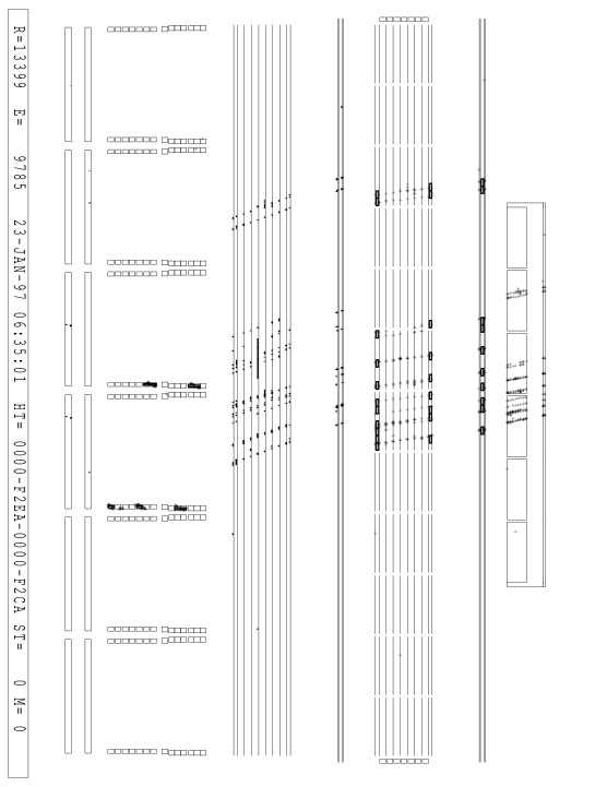
Figure 5.1: A two cluster event detected by MACRO as seen with the event display of the experiment.

The two methods can be regarded as “complementary”. Both methods have the common feature to look for correlations between muons inside the bundle, but in a different way. With the first method we study the core of the bundle, which is densely populated with high energy muons. We will see how this feature can be used to perform a composition study. The second method, on the contrary, is most suitable to study the “peripheral” region of the bundle, composed of isolated muons generated in the very first interactions of the shower development. These muons can provide informations on the interaction model. Fig. 5.2 explains this concept: using the Monte Carlo HEMAS we computed the mean number of muon parent generations as a function of the muon distance from the shower axis. The contributions of pure Proton and pure Iron primaries are well separated. We observe three features: (i) iron primaries have a different behaviour than protons; (ii) near the shower axis the mean number of generations is larger with respect to muons far away from the axis; (iii) in the limit of very large distances from the axis, the muons come from mesons of the first interactions, independently of the primary type.

Figure 5.2: Average number of generations in atmosphere to produce muons at the detector level obtained with the Monte Carlo HEMAS. The contributions of Iron and Proton primaries are separated.

We stress that these analyses have to face with two problems of different nature:
(a) The study of correlations between muons inside the bundle requires a selection of relatively high multiplicity events. We know for higher muon multiplicities the event rate is lower. Moreover, we expect that if a correlation signal exists in the data, it will be of the order of few percent. In fact, muon bundles observed underground are produced in nuclear interactions at several kilometers up in the atmosphere by primaries of different energies, by different types of primaries and at different slant depths: the sum of all these effects smoothes the signal in the background of statistical fluctuations. Very roughly, we can observe from the MACRO multiplicity distribution of Fig. 1.3 that there is a factor $\sim 2\times 10^{-4}$ between the number of single muon events and the number of events with $N_{\mu}$$\geq$ 8. Considering a total number of $\sim 2\times 10^{7}$ muon events, we have $N_{\mu}\sim$ 4000 events with a multiplicity $\geq$ 8 and a ratio $\delta N_{\mu}$/$N_{\mu}$ $\sim$ 2%.

From an experimental point of view, it is not possible to associate in the wire and strip views all the muons belonging to high multiplicity events. When the multiplicity is high, the muons are very close the one another and the geometry of the event cannot be reconstructed in a non-ambigous way using the informations of both the wire and strip views. So we are forced to use only one projective view (the wire view).

(b) Any correlation study requires the comparison between the experimental sample of events and a second sample of uncorrelated events. This second sample is usually derived from the first one by mixing the particles between different events (“event mixing”) or is computed in an analytical way, considering the functional form of the distribution of the particle. This is not our case: the distribution of the particles in the bundle is different from event to event. For instance, the functional form of the muon positions inside the bundles depends on the primary types, primary energy, muon production heights etc. We are then forced to use different approaches, which we shall discuss in the following.

5.2 Event selection

In this analysis we used the data taken in the period July 94 - December 98 with the apparatus in its final configuration (six supermodules, lower part and attico). We required a good quality of the runs with the following cuts:
(a) Run lenght $\geq$ 1.5 hours;
(b) Dead time for each $\mu$VaX $\leq$ 2.0%;
(c) $\epsilon_{wire}\geq$ 83%, $\epsilon_{strip}\geq$ 70% (for each module);
(d) muon number $N_{\mu}$ in the limits: $840\leq N_{\mu}\leq 960$;

The main differences with respect to the decoherence analysis are the points (b) and (d), both connected with the introduction of the attico. The point (c) assures a perfect performance of the whole detector. The total live time with this selection is $\sim$ 21622 h corresponding to about $2\times 10^{7}$ muon events. We selected the events according to the following cuts:
(e) number of muon tracks reconstructed in the wire view $N_{wire}\geq$ 8;
(f) parallelism requirement between tracks;
(g) zenith angle $\theta\leq 60^{\circ}$;

Before the event selection, we required, for each reconstructed track, hits in at least four planes of the lower part of the apparatus. This ensures a good quality of the events and prevents the inclusion of fake tracks due to e.m. processes in the top of the apparatus. The total number of multiple muon events which survive to these cuts is 4893.

Figure 5.3: Distribution of primary cosmic ray energy per nucleus relative to underground muon bundles with $N_{wire}\geq$ 8 (HEMAS/DPMJET Monte Carlo).

5.3 Monte Carlo simulation

The requirement of muon wire multiplicity $N_{wire}\geq$ 8 is a strong selection on primary cosmic ray energies. We used the complete simulation with the HEMAS hadronic interaction model to estimate the minimum primary energy corresponding to this selection. We estimated that the number of events reconstructed with $N_{wire}\geq$ 8 and with a primary energy $E_{nucleus}$ $<$ 1000 TeV is less than 1%. We obtained the same result from an independent production performed with the DPMJET-II.3 interaction model (see Fig. 5.3). Moreover, Fig.6 of Ref. [12] shows that this result does not depend on the composition model adopted.

This is an interesting feature, since a complete production with a minimum energy of 1000 TeV is not very CPU time consuming, and it is possible to produce a complete simulation for each hadronic interaction model. We have generated a complete production for each of the Monte Carlo configurations given in Tab. 5.1. For each production 156830 primaries have been simulated according to the “overall” spectrum for a total live time of 5528 h (see Tab. 5.2).

Interaction	Shower Propagation	Number of survived	CPU time
Model	Code	events $N_{\mu}\geq$ 8	(sec/event)
HEMAS	HEMAS	13386	3.6
DPMJET-II.3	HEMAS	14419	9.0
DPMJET-II.4	HEMAS	15148	8.9
QGSJET	CORSIKA	11616	5.5
SIBYLL	CORSIKA	10918	1.9
HDPM	CORSIKA	11585	1.6

Table 5.1: Monte Carlo simulation set up. For each Monte Carlo configuration (hadronic interaction model and shower propagarion code) we give the number of survived muons $N_{\mu}\geq$ 8 and the CPU time in seconds required to process one event.

Primary	Primary	Number of events
Type	Energy	generated according
	(teV)	to the overall model
P	1000–100000	52567
He	1000–100000	17028
CNO	1000–100000	15761
Mg	1000–100000	10501
Fe	1000–100000	60973

Table 5.2: Statistical sample of the MC productions performed for each of the MC configuration of Tab. 5.1. In correspondence of each energy band, we give the number of generated events according to the “overall” model.

In the first two columns of the table are reported the set-up of the Monte Carlo configurations adopted. We used the hadronic interaction models HEMAS [31], DPMJET-II [35], QGSJET [51], SIBYLL [52], HDPM [47] and the shower propagation codes HEMAS-DPM [33] and CORSIKA [32]. The CORSIKA shower propagation code, which is generally used for EAS array and surface experiments, has been interfaced with the routine set of the HEMAS code. The output of the CORSIKA code, which is given in a different reference frame with respect to the HEMAS one, has been properly tranformed to be inserted in the muon propagation code PROPMU [54]; in this way, the output of the two shower propagation codes have the same format and can be processed using the same tools. The GMACRO and DREAM codes have been used to reproduce the detector effects. In the third column of Tab. 5.1 is reported the number of survived events $N_{\mu}\geq$ 8 at the detector level before detector simulation (“overall” model). The last column indicates the CPU time used expressed in sec/event. (The simulation has been performed on a DIGITAL UNIX platform, Ultimate Workstation, 533 au2, 16.6 SPECint95 for each CPU).

To spead up the simulation procedure, each particle produced in the atmosphere has been followed up to a threshold energy computed considering the event direction and the actual amount of rock to cross. This energy has been deduced in an empirical way and the used relation is :

$$E_{\mu}^{min}(TeV)\simeq 0.66\,\times(e^{0.29X}-1)$$ (5.1)

where $X$ is the rock thickness expressed in Km w.e. It has been estimated that the error obtained using this approximation is less than $10^{-4}$.

In the following we are interested in high multiplicity events. It is important to check that the sample of experimental and simulated events are homogeneous. Actually, we know that for very high multiplicity events ($N_{wire}$ $>$ 15), the tracking package fail the track reconstruction. This happens when the hit density of the events is very high and after several iteration the tracking algorithm is not able to find the best pattern configuration. In this case, the code marks the events with a “label” and they can be analysed using different procedures. The problem is that the “starting point” in the multiplicity distribution where the tracking starts to fail may be different for the real and simulated data. The reason is that the thin differences between the real and simulated detector parameters are crucial for high density events. For instance, the simulation of the background noise or the cluster widths are parameters which can affect the pattern recognition of the tracking algorithm. During the last years, the detector simulator has been improved and the parameters have been tuned to the real data in order to reproduce a detector response as realistic as possible. Nevertheless, some difference are still present and this may introduce some biases in the following analyses. There are two ways to proceed:

$\bullet$ the first approach has been followed in [80]. The events labelled by the tracking are visually scanned and the parameters of the best bundle configuration are written in a separated file. This sample of event is merged with the first sample and can be analysed as a whole;

$\bullet$ the alternative is to introduce a cut in the multiplicity distribution where the contribution of the failed events is negligible both for the real and the simulated data.

Event	Visually	Reconstructed	Reconstruction
multiplicity	scanned events	events	efficiency
8	0	594	100
9	0	364	100
10	0	249	100
11	0	155	100
12	1	110	99.1
13	7	83	91.6
14	2	46	95.6
15	5	37	86.5

Table 5.3: Event statistics for a sample of visually scanned events. We give the number of scanned events, the number of reconstructed events and the reconstruction efficiency as a function of the multiplicity.

	Number of survived
	events in the range
	8 $\leq N_{wire}\leq$ 12
REAL DATA	4514
HEMAS	3930
DPMJET-II.3	4196
DPMJET-II.4	4470
QGSJET	3529
SIBYLL	3094
HDPM	3179

Table 5.4: Final statistics for the events used in the analysis. The number of experimental events and simulated events is relative to different livetimes (see text).

Considering the large statistical sample available, we are forced to use the second approach. To estimate the maximum value of the event multiplicity we can include in the analysis, we used the scanned events of a limited statistical sample of real data and simulated data. In the sample of simulated data, all the events up to $N_{wire}$ = 15 were successfully reconstructed by the standard tracking. In the sample of real data, the situation is shown in Tab. 5.3 where we report, as a function of the multiplicity, the number of events visually scanned, the number of events reconstructed by the tracking algorithm, and their ratio in percentage. We choose as maximum value of multiplicity to include in the analysis $N_{wire}^{MAX}$ = 12. In this case the number of not reconstructed events is less than 1% both for the real and simulated data. In the following, if not stated otherwise, the results are given in the multiplicity range 8 $\leq N_{wire}\leq$ 12. In Tab. 5.4 we give the final statistics for real and simulated events. We observe that the numbers relative to the Monte Carlo simulations differ considerably for the different Monte Carlos. This result is connected with the charged multiplicity yield at generator level (see for instance Tab. 21 and Tab. 27 of Ref. [70]).

5.4 Correlation Integral analysis

5.4.1 Generalities

The study of fluctuations in particle physics has a long history. In the ’80s, the JACEE collaboration [82] reported the observation of an event with high density “spikes” in the rapidity distribution. They observed that single events presented strong density fluctuations compared with average distributions. This phenomenon was later observed also in $p$-nucleus and hadron-hadron interactions. The interest in this field is connected with the possible quark gluon plasma formation in heavy ion collisions or with the study of intermittency of the parton showers in multiparticle production processes. The common feature of these studies is the scale invariance and self-similar behaviour of the processes involved. This property is called “multifractality”. Cascade models (or branching models) are natural candidates to describe physical processes where a multifractal behaviour is present (a general review on this subject can be found in Ref. [83]).

The idea to apply this analysis method to cosmic ray physics rises from the observation that cosmic ray air showers are typical cascade processes. We know that showers originated by different primaries develop in atmosphere in different ways (see for instance Fig. 5.2). If muon bundles detected underground preserve “memories” of the showering processes in the atmosphere, the study of density fluctuations inside muon bundles could give information on the primary cosmic ray composition. Hadronic interaction models should have, in first approximation, little influence on the shower “pattern” in the atmosphere, since this is mainly determined by the mean free paths and decay lengths of parent mesons. The average muon displacement due to Coulomb scattering in the rock is $\sim$ 50 cm if we consider muons near the shower axis, where the residual muon energy is larger with respect to peripheral muons (Fig. 5.4). In the limit of very large distances from the shower axis, the average muon displacement is is $\sim$ 250 cm asymptotically. Therefore, if a correlation pattern exists at the atmospheric level, part of this pattern can be recovered underground if we consider the core region of the bundle.

Figure 5.4: Average energy of muons which arrive at the detector level. The black point are the energy in atmosphere (before entering in the mountain) while the white points indicate the residual energy underground. Note that the mean muon energy in atmosphere is larger than the single muon energy (1.4 TeV at threshold), reflecting the high primary energy of this event sample.

5.4.2 The method

Presently, the best method to study anomalous density fluctuations is the so called factorial moment analysis. The method was introduced in particle physics by Bialas and Peschanski [84] as a tool to look for intermittency in heavy ions collisions. Suppose to have a 1-dimensional variable $y$ which characterizes a set of points (the extension to multi-dimensional variables is straightforward) with distribution $\rho_{1}(y)$ in a given domain $\Delta y\equiv\Omega$. Fundamental in this analysis is the concept of inclusive q-particle distribution $\rho_{q}(y_{1},...,y_{q})$ which is connected with the probability to find simultaneously one point in $y_{1}$, one in $y_{2}$ etc. In multiparticle physics these distributions are given by:

$$\rho_{q}(y_{1},...,y_{q})=\frac{1}{\sigma_{inel}}\frac{d^{q}\sigma_{incl}}{dy_{1}...dy_{q}}$$ (5.2)

where $\sigma_{inel}$ is the inelastic cross section, $\sigma_{incl}$ is the inclusive cross section and $y$ denotes the rapidity. In general, the experimental procedure to determine $\rho_{q}$ is the following: from each event of multiplicity $n$, take all the possible ordered q-tuples $\{y_{i_{1}},...,y_{i_{q}}\}$ and add 1 at the position $(y_{i_{1}},...,y_{i_{q}})$ of the q-particle distribution. Repeat the procedure for all the $n(n-1)...(n-q+1)\equiv n^{[q]}$ ordered q-tuple and average over the whole event sample. The quantities $n^{[q]}$ are called factorial moments of the distribution. Note that for an uncorrelated event sample the q-particle distribution factorizes:

$$\rho_{q}(y_{1},...,y_{q})=\rho_{1}(y_{1})...\rho_{1}(y_{q})$$ (5.3)

which defines an uncorrelated Poisson process. The integrals of the left and right side of Eq. 5.3 are, respectively:

$$\int_{\Omega}{dy_{1}...dy_{q}\rho_{1}(y_{1})...\rho_{1}(y_{q})}=\langle n^{[q]}\rangle_{\Omega}$$ (5.4)

$$\int_{\Omega}{dy_{1}...dy_{q}\rho_{1}(y_{1})...\rho_{1}(y_{q})}=\langle n\rangle^{q}_{\Omega}$$ (5.5)

This means that the factorial moments of a purely statistical distribution is the average number of particles in $\Omega$ and can be used to normalize the (non statistical) factorial moments. The idea of Bialas and Peschanski was to study the behaviour of factorial moments in ever-decreasing cells of the domain space. Here we use a recent development of this method, called correlation integral (or strip integral) [85]. These are defined in the following way:

$$C_{q}(\delta y)\equiv\frac{\int_{\Omega(\delta y)}{dy_{1}...dy_{q}\rho_{q}(y_{1}...y_{q})}}{\int_{\Omega(\delta y)}{dy_{1}...dy_{q}\rho_{1}(y_{1})...\rho_{1}(y_{q})}}$$ (5.6)

where $\Omega(\delta y)$ is the q-dimensional domain space which varies according to the resolution parameter $\delta y$ (Fig. 5.5). In practice, we count the number of q-tuple which have a distance $\leq\delta y$. The “distance” of a q-tuple with q $>$ 2 is determined according to the GHP convention [86]: we require that all the possible pairs of points inside the q-tuple have distances $\leq\delta y$. In the case of q=2, this corresponds to count the number of pairs which are included in the strip domain $\Omega$ of Fig. 5.5. In this work, we will use only the case q=2 and q=3, since larger orders of the correlation function require a very high multiplicity per event.

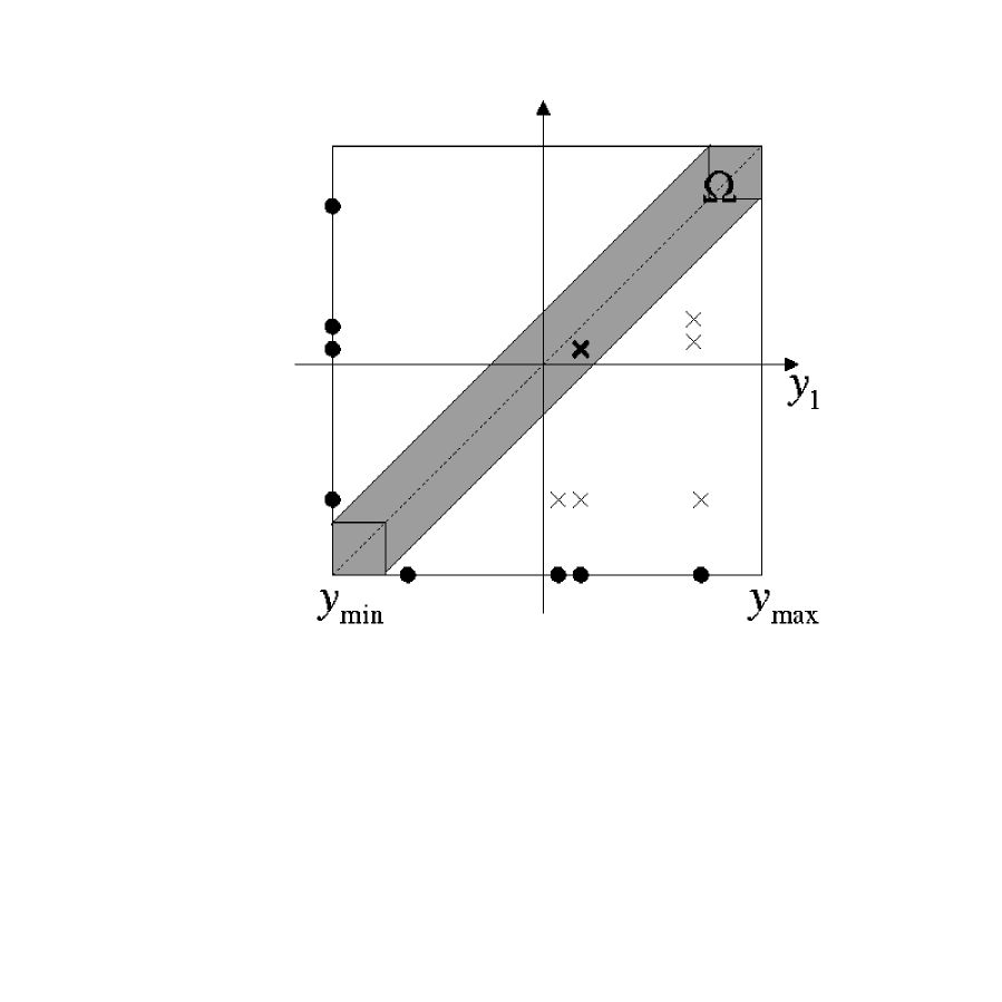
Figure 5.5: Integration domain for the correlation integral. It is shown the case for an 8-muon event and the strip relative to a scale parameter $\delta y$.

The normalization of the correlation integrals (the denominator of Eq. 5.6) can be performed in two different ways: in the so called vertical normalization the denominator is computed using an uncorrelated event sample built ad hoc; the horizontal normalization uses an analytical computation of the strip volume:

$$\Omega(\delta y)=q\Delta Y(\delta y)^{q-1}-(q-1)(\delta y)^{q}$$ (5.7)

In this kind of analyses, the results are generally given in double-log plots because, if a self-similar behaviour is present in the data, it has a functional form:

$$C_{q}(\delta y)\propto(\delta y)^{\alpha_{q}}$$ (5.8)

corresponding to a straight line in double-log plots. An uncorrelated event sample is characterized by an horizontal line ($\alpha_{q}$ = 0 for all q).

5.4.3 The results

Before applying the method to our experimental data, we checked how this method is sensitive to the development of the shower in the atmosphere. We used a simple toy model, inspired from the branching $p$ model [88], to understand the influence of the number of particle generations on the self-similarity of the pattern we observe. This model must show a self-similar behaviour by construction. We generated 10000 events at fixed multiplicity $m=8$ in the domain $\Delta Y$ = 10000 cm in the following way. For each particle $i$ in the event:
1) chose a given number of steps $K$;
2) at each step, divide the domain $\Delta Y$ in two parts;
3) choose randomly one of the two segments;
4) repeat steps 2 and 3 up to the number of steps $K$;
5) choose randomly the position of the particle in the segment of length $\Delta Y/2^{K-1}$.
Repeat the steps 1-5 for all the 8 particles in the event. In Fig. 5.6 we show the results. We plot the correlation integrals (with the horizontal normalization) for q=3 and for different values of $K$ as a function of the scaling parameter $\delta y$. We see that the self-similar pattern is almost completely hidden for low $K$ values, while it becomes clear as $K$ increases. For $K$ = 10 we see a complete scaling law at all distances. From this exercise, we can conclude that, even if we deal with a pure self-similar system, the number of steps in the generation of the pattern affects the final result. This is the main feature we exploit to discriminate the primary cosmic ray mass in this analysis.

Figure 5.6: Correlation integral of third order (q=3) relative to the toy model explained in the text. The behaviour of the scaling law is shown as a function of the number of steps (generations) from $K$ =1 up to $K$ = 10.

We computed the correlation integral for the experimental data according to Eq. 5.6 for q=2 and q=3. For each event, the “center of mass” was computed as

$$\langle x\rangle=\sum_{(i=1)}^{m}(x_{i}-\bar{x})$$ (5.9)

where $m$ is the multiplicity of the event, $x_{i}$ are the muon positions in the wire view and and $\bar{x}$ is the average value. This variable is a good estimator of the axis of the bundle. Using the HEMAS Monte Carlo, we proved that in the wire view the average distance from the “real” shower axis and the one reconstructed using Eq. 5.9 is (143$\pm$2) cm. We selected a window around $\langle x\rangle$ of $\Delta Y$ = 1000 cm. To avoid the inclusion of the contribution from muons originated in the pair production processes discussed in the previous chapter, we place a cut of 1m in the muon distance. If a muon pair in the selected region had a separation $d>$1.5m, one of the two muons, randomly chosen, was erased from the event and correspondently the multiplicity of the event was decreased by one unit. This cut is important in the core region where the muon energies involved are much larger with respect to the rest of the bundle.

Figure 5.7: 2nd and 3rd order correlation integrals of the experimental data as a function of the scaling parameter. The data have been normalized with the light model (above) and with the heavy model (below).

To normalize the correlation integrals, we used the vertical normalization. In particular, we used the Monte Carlo data for each composition model (“heavy”, “light” and MACRO-fit model) to compute the denominator of Eq. 5.6. In this way, we can measure the relative amount of correlations in the data comparing them to those predicted by different composition models. For instance, we expect that if compared with an iron rich composition model, the data exhibit the maximum correlation pattern. In Fig. 5.7 we show an example of the correlation integral $C_{2}$ and $C_{3}$ for the experimental data normalized using the HEMAS Monte Carlo with the light (above) and heavy (below) composition models.

For each Monte Carlo configuration and for each composition model, we performed a best fit to a straight line for plots similar to those Fig. 5.7 to extract the indexes $\alpha_{q}$. In Fig. 5.8 we present the indexes $\alpha_{2}$ and $\alpha_{3}$ for each Monte Carlo (above plots) and a summary plot where the same values are reported in the plane ($\alpha_{2}$,$\alpha_{3}$). We did not include the HDPM Monte Carlo configuration because of convergence problems during the fit procedure. We observe that, even if the two extreme composition models behave differently when the interaction model is changed, the MACRO-fit model is preferred by the experimental data, independently of the interaction model adopted. Even if the agreement is not perfect inside the statistical errors, we can be confident in using the MACRO-fit composition model to extract informations on the hadronic interaction model.

Figure 5.8: Correlation integral indexes $\alpha_{2}$ and $\alpha_{3}$ for the experimental data normalized with different Monte Carlo configurations and different composition models. In the plots above $\alpha_{2}$ and $\alpha_{3}$ are plotted for each Monte Carlo. Above, the results are shown in the $\alpha_{2}$ and $\alpha_{3}$ plane.

5.5 Cluster analysis

5.5.1 Generalities

The search for substructures inside muon bundles is a new method for the analysis of multiple muon events introduced for the first time in Ref. [79, 80, 81]. The results, although preliminary, have shown that the method is sensitive both to the hadronic interaction model and to the chemical composition of primary cosmic rays at the same time. The study of the clustering inside muon bundles shares the same conclusions obtained with the multiplicity distribution and the decoherence function separately, even if the method cannot disentangle the two effects. Moreover, it was pointed out that the method could give additional informations with respect to the traditional methods. The reason is that if the clustering that we observe underground is correlated with the shower development in the atmosphere and/or with the feature of the hadronic interaction model, a study on how these clusters occur can offer a test of the details of the simulation programs we use. From a technical point of view, the search for substructures is performed by means of software algorithms. The choice of the algorithms is a delicate step of the analysis: depending on what one expects to find, there exists an optimized algorithm for the purpose. Exploiting a set of algorithms commonly used in the literature, we will look for the algorithms which better fit our purpose.

We expect that most of the substructures observed underground are the result of statistical fluctuations on the position of the muons with respect to their average values. In general, any set of points with a given distribution gives rise to a cluster structure when a clustering algorithm is applied. A difficult task is to understand if there is an additional clustering of dynamical origin in the data, other than the trivial statistical one.

5.5.2 A first check on the interaction models

Figure 5.9: Ratio between the experimental and simulated decoherence functions for the sample of $N_{wire}\geq$ 8. The ratio was computed between distributions normalized to the same number of events.

Figure 5.10: Ratio between the experimental and simulated decoherence functions for the sample $N_{wire}\geq$ 8. The ratio has been computed between distributions normalized to the same number of events.

Before introducing this method, we study the decoherence function in the wire view for the selected high multiplicity events. Following the formalism of the previous Section 4.1, we compute for each event the distances of all the $N_{wire}(N_{wire}-1)/2$ pairs in the event. In Fig. 5.9 we give the ratio of the experimental decoherence function to the simulated ones (normalized to the same number of event) as a function of muon separation. For each interaction model the MACRO-fit model has been used. In Fig. 5.10 we show the same plots with a different binning to explore the high distance region up to the maximum value allowed by statistics ($\sim$ 40 meters). In the low-medium distance region there is a general distortion of the decoherence curve for all the models considered, in particular DPMJET, even if the effect is less than 10%. This is not surprising because in this analysis we did not apply all the refined cuts discussed in the previous chapter. A more detailed analysis in the low-medium distance region requires the subtraction of the background due to local hadro-production and muon pair production by muons. Here we are interested in the tail of the distributions, where these background processes are not important. We can thus isolate the very high energy contribution to the total decoherence function $N_{\mu}\geq 2$ and test the $P_{T}$ modelling of the different hadronic interactions for $E_{primary}\geq$ 1000 TeV. The results show that DPMJET and QGSJET are the two MC codes which better reproduce the experimental data. HEMAS and HDPM seem to overestimate the experimental distribution for distances D $>$ 30 meters, while SIBYLL underestimates by a factor of three.

5.5.3 Clustering algorithms

The choice of the clustering algorithm is a crucial point in searching for a signal of dynamical origin. Cluster analysis is a wide branch of statistical sciences and its application run over many different fields (for a good introduction to cluster analysis see [89]). There are many cluster algorithms in the literature. In Ref. [90] there is a classification of the most used algorithms. In particle physics, data clustering is connected with the search for substructures in multi-jet events at colliders. The most popular jet finding algorithm was introduced by the JADE collaboration [91].

Clustering algorithms can be classified into two main classes:

(a) Partitioning Algorithms. In these algorithms, the user decides a priori the number of clusters in which the data must be grouped. The algorithms then perform all the possible combinations of points to find out which is the best configuration according to some specified criteria (for instance the minimization of the inter-particle distance in the same cluster). This class of algorithms is not suitable for our purposes: we do not know a priory the number of clusters in which an event must be divided.

(b) Hierarchical Algorithms. Hierarchical Algorithms do not fix the number of clusters but consider all possible number of clusters in a single event. For instance, if we have an event with $M$ particles, the algorithms start to group the particles from the configuration with the maximum number of clusters ($N_{cluster}$ = $M$). At each step, two clusters are merged together according to some criteria, until the configuration $N_{cluster}$ = 1 is reached at the $M$-th step. These are called agglomerative hierarchical algorithms. The divisive hierarchical algorithms start from the configuration $N_{cluster}$ = 1 and at each iteration a cluster is splitted in two parts until the configuration $N_{cluster}$ = $M$ is reached at the $M$-th step. The divisive algorithms are very CPU time consuming, because at each iteration all possible combinations must be computed. So in this analysis we use the agglomerative hierarchical algorithms only.

Agglomerative Hierarchical algorithms

Agglomerative Hierarchical Algorithms differ one from another in the way they compute the distances between the clusters. The two clusters separated by the smallest distance are merged. In this work we use four different types of algorithms:

1) centroid method: the distance between two clusters is defined as the distance between their centroids (“center of mass”). The centroid coordinates of a cluster C is defined as:

$$X_{C}^{d}=\frac{1}{M_{C}}\sum_{i\in C}x_{i}^{d}$$ (5.10)

where $M_{C}$ is the multiplicity of the cluster and $d$=${1,...,D}$ is the dimension index ($D$ = 1 if we work in a projected view). For this algorithm we use the same convention of Ref. [79, 80, 81]: the distance between the clusters is the centroid distances multiplied by a factor that takes into account the multiplicity of the clusters

$$\chi_{AB}=(N_{A}N_{B})^{0.25}*R_{AB}$$ (5.11)

where $M_{A}$ and $M_{B}$ are the multiplicity of the clusters and $R_{AB}$ is the euclidean distance between the clusters.

2) single linkage: the distance between two clusters A and B is defined to be the minimum of the Euclidean distances between all the pairs of points with one point in A and one point in B;

3) complete linkage: the distance between two clusters A and B is defined to be the maximum of the Euclidean distances between all pairs of points with one point in A and one point in B;

4) Ward’s procedures: at each iteration, the within-cluster sum of the squared deviations about the centroid is computed

$$S_{C}=\sum_{d=1}^{D}\sum_{i\in C}(x_{i}^{d}-X_{C}^{d})^{2}$$ (5.12)

The merging is chosen to minimize $S_{C}$.

In Fig. 5.11 are represented in a naive form the inter-cluster distance definitions used in this work. Note that in all the four algorithms a cluster can be composed by a single particle. In the following, we refer to the four algorithms 1,2,3 and 4 with the names “H1”, “H2”, “H3” and “H4”, respectively.

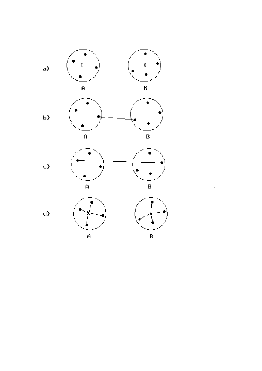
Figure 5.11: Representation of inter-cluster distances for the methods used.

At each iteration, the number of clusters decreases by one unit until it reaches $N_{cluster}=1$. How can we decide when to stop the algorithm and remain with a given number of clusters ? There are two ways to proceed:

(a) We can stop the algorithm when the “distance” between the two last merged clusters is larger than a fixed value. We will refer to this choice as sharp clustering;

(b) More interesting is the so called natural clustering. This approach is usually used in pattern recognition studies, which attempt to reproduce the human eye behaviour. For instance, the event shown in Fig. 5.1 seems to be “naturally” formed by two substructures. Any hierarchical algorithm can be properly described by a dendrogram, which is a graphical description of the iteration process. This is shown in Fig. 5.12 for an event with multiplicity $M$ = 8. On the horizontal axis is reported the value (“depth”) at which a cluster merging occurs. From the left of the picture, we observe that at each iteration the cluster number decreases by one. To define a natural clustering, we consider the depth $d_{j}$ at which the $j$-th merging occurs; if the ratio:

$$R_{nat}=d_{j}/d_{j-1}$$ (5.13)

if greater than a fixed value $\bar{R}_{nat}$, we say that the configuration $N_{cluster}$ = $M-j+1$ is the natural clustering of the event. For instance, the event of Fig. 5.1 has been selected using the algorithm H3 with a natural clustering $\bar{R}_{nat}$=4. One of the main advantages of the natural clustering is that it leaves out any dependence from the different scales of the events. By construction, the natural clustering considers relative variables in the events (see Eq. 5.13) and not absolute values.

The application of the four algorithms to the same data sample produces different outputs. We do not know a priori how and if the clustering inside multiple muon events occur, so we have to apply all the algorithms. The main difference between the four algorithms is in the topological clustering selection they perform on the events. For instance, algorithm H2 usually looks for well elongated and far away clusters, while the algorithm H3 selects compact and close clusters.

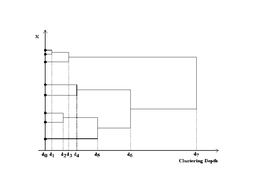
Figure 5.12: A Dendrogram relative to the clustering of an eight muon event.

5.5.4 Dependence on the composition model

The sensitivity of the method on the primary composition model has been tested in Ref. [79, 80, 81]. We have used the HEMAS MC configuration and three different composition models: the “MACRO-fit” model [15, 16], the “light” and the “heavy” models [6]. In Fig. 5.13 we have plotted the fraction of events with 1 and 2 clusters as a function of the scaling parameter $\chi_{cut}$ after the application of the H1 algorithm.

Figure 5.13: Fraction of events reconstructed as 1 and 2 clusters for the experimental data and simulated data with different composition models. The algorithm H1 has been applied.

We observe two features:

- The method is sensitive to the composition model. In particular, a heavier composition produce events with more clusters with respect to a lighter model;

- The MACRO fit model is the one that better reproduces the data.

We argue that the sensitivity of the method to the primary composition model is mainly connected with the different event scale produced by heavy primaries with respect to light primaries. Heavy primaries have a large cross section and the first interaction point is higher in the atmosphere. Therefore, muon bundles produced by heavy primaries have on average a larger muon pair separation with respect to the ones produced by protons. To better exploit this point, we fix the multiplicity of the events (e.g. $N_{wire}$ = 8). In this way, we get rid of any multiplicity effect. As in the previous section (Eq. 5.9), we compute for each event the absolute first order momentum (“center of mass”) $\langle x\rangle$, a quantity closely connected with the average value of the function $f(r)$, the distribution of muon distances from the shower axis. In Fig. 5.14 we show the normalized distribution of $\langle x\rangle$ for the simulated light and heavy composition models.

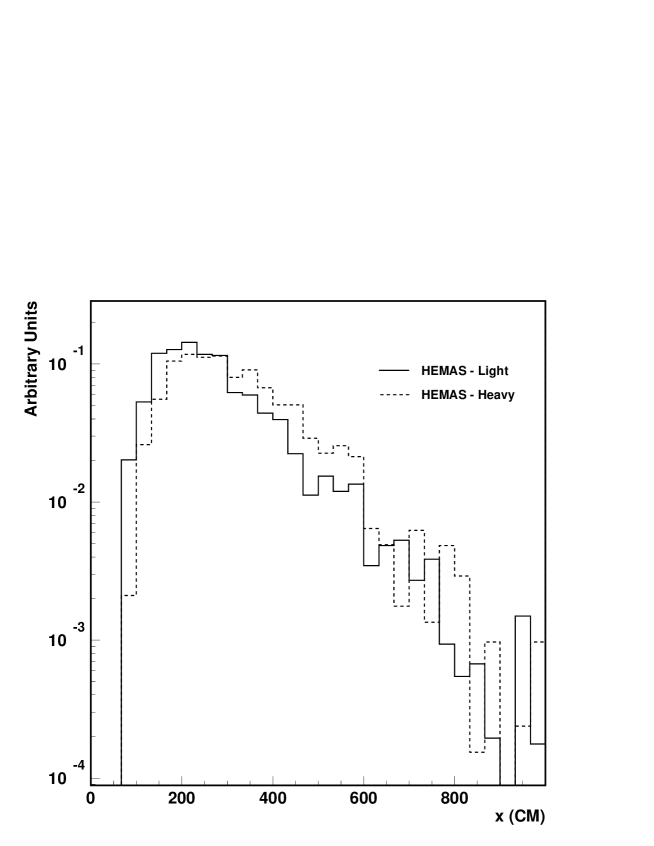
Figure 5.14: Monte Carlo simulation: distribution of the $\langle x\rangle$ value (see text) for the light and heavy composition model for muon events of fixed multiplicity $N_{wire}$ = 8.

As we expected from the study of the decoherence function, the two distributions are similar: the “volume” of the events is in first approximation independent from the composition model. But the difference that we observe in the two histograms ($\sim(10\pm 1)\%$ in the average values) is enough for the cluster method to discriminate between the two models. We have to prove the following hypotheses:
(a) the cluster analysis is sensitive to small differences of densities;
(b) the composition dependence that we observe at fixed multiplicity is due uniquely to this difference and not to a topological difference in the events.

In order to discuss the first point, we use a simple toy model. We generate 10000 events in a 1-dimensional space with a flat distribution in the range $[0-1]$ at a fixed multiplicity $m$ = 8. We then perform a density variation of 5%: we generate another sample at fixed multiplicity $m$ = 8 in the range $[0-1.05]$. In Fig. 5.15 are shown the results after the application of the algorithm H1. It is clear that the method discriminates the two samples. This sort of “amplification” effect of the method for small density variation is hidden in the mathematical structure of hierarchical clustering algorithms .

Figure 5.15: 1-2-3 cluster fractions for an event sample generated with a toy model at fixed multiplicity $N_{wire}$ = 8 (algorithm H1).

The effect due to the different event densities can be erased re-computing the muon positions using the transformation:

$$x_{i}^{{}^{\prime}}=x_{i}\frac{\langle x\rangle}{\langle x\rangle}_{TOT}$$ (5.14)

where $x_{i}$ ($i=1,m$) is the original position of the $i$-th muon in the event, $\langle x\rangle$ is the absolute event average and $\langle x\rangle_{TOT}$ is the absolute average for the total event sample. Each event has now the same density; an eventual difference in the clustering plots is due to an intrinsic difference between events generated by different primaries. The result is shown in Fig. 5.16: we observe that the composition dependence has been deleted.

Figure 5.16: 1-2-3 cluster fractions for rescaled (simulated) events at fixed multiplicity $N_{wire}$ = 8 (algorithm H1).

A different and more direct way to reach this conclusion is to consider the natural clustering. Without and coordinate transformation, this method allows to explore the intrinsic event structure. This is shown in Fig. 5.17 where we used the H4 algorithm. In the left part is shown the clustering rate plots with the sharp clustering for event at fixed multiplicity $m=8$; in the right side are reported the cluster rate of the same event sample. We observe that any composition dependence disappears if we look at the event intrinsic event topology using the natural clustering. We can conclude that the intrinsic event structure as seen with these methods does not depend on the primary cosmic ray mass. Here we used the HEMAS interaction model: we obtain the same results using all the four clustering methods for each of the interaction model considered in this work.

Figure 5.17: 1-2-3 cluster fractions as seen with the sharp clustering, above, and with the natural clustering, below (algorithm H3).

5.5.5 Dependence on the hadronic interaction model

Following the scheme of the previous section, we test the dependence of the method on the hadronic interaction model in two steps. First we plot the cluster fractions without any scaling of the events. In this way we check how the event density is reproduced by different interaction models. A correct reproduction of the experimental event density is a robust test of the Monte Carlo reliability in reproducing the shower development as a whole, being this density the convolution of different and competing factors. In the second steps we analyse the intrinsic topology of the events in a scale-independent way: our aim is to isolate the pure contribution of some of the hadronic interaction features.

Event density sensitivity

We start comparing in Fig. 5.18 the cluster fractions of the experimental data with the ones obtained using the NIM85 and HEMAS interaction models (for the “light” composition model). It is clear that the behaviour of the two models is completely different, and that the NIM85 is the one that disagrees with the data. The reason is not in the different intrinsic topology of the events. NIM85 is not able to reproduce the lateral shape of the events observed in MACRO, as the decoherence analysis has shown in the past [62]. This feature is amplified in this analysis. NIM85 does not include a power law component in the modelling of the transverse momentum, which is fundamental in reproducing the high $p_{t}$ tail of the distribution observed at colliders. This feature results in narrower muon bundles underground; consequently in larger fractions of one cluster events, at fixed $\chi_{cut}$. Again, we observe how this method is able to “amplify” small event density differences.

Figure 5.18: 1 and 2 cluster fraction (algorithm H1) for the experimental data and for the simulated data obtained with the HEMAS and NIM85 interaction models (light composition model).

Figure 5.19: 1 and 2 cluster fractions (algorithm H1) for the experimental data and for the simulated data obtained with different Monte Carlo codes (MACRO-fit model).

Figure 5.20: 2-cluster events ratio of experimental data over simulated data. The plots on the right refer to events reconstructed with a central cluster plus an isolated muon; on the right side: events reconstructed with a central cluster plus a cluster with at least two muons.

Let us now consider the hadronic interaction models presented in Tab. 5.1. In Fig. 5.19 we compare the cluster fractions of the experimental data with those of simulated ones using these interaction models and the MACRO-fit composition model. Now the agreement is good and all the models reproduce quite well the shape of the experimental data. This implies that all the models considered reproduce in first approximation the right density of muon bundles. A more detailed study of Fig. 5.19 shows that the agreement is not perfect for all the interaction model considered. For instance the DPMJET and HDPM models overestimate the 2-cluster fraction around $\chi_{cut}$ = 1200 cm and $\chi_{cut}$ = 2000 cm respectively.

To better understand the behaviour of the plots for high values of the parameter $\chi_{cut}$ (where the fraction of 2-cluster event is small), we plot in Fig. 5.20 the ratio of the 2-cluster fractions experimental data/Monte Carlo as a function of $\chi_{cut}$. Moreover, we separate the samples of 2-cluster events into two sub-samples: events reconstructed by the H1 algorithm as 2-cluster events with one of the clusters formed by a single muon (sample A); events reconstructed by the H1 algorithm as 2-cluster events with one of the clusters formed by at least two muons (sample B).

The result is strictly connected with the result of Fig. 5.10: in the high value of the parameter $\chi_{cut}$ (i.e. far away from the shower axis), the data are correctly reproduced by the QGSJET model, while DPMJET, HEMAS and HDPM overestimate these events and SIBYLL underestimates them. In this case we can add some information: the disagreement with the data is due to events with a central cluster and an isolated far away muon. In the next section we show that, with the exception of SIBYLL for which the discrepancy is of a topological nature, these results are due to the different event scales.

Topological event structure

In this section, we are going to search for clustering of dynamical origin inside muon bundles. The number of clusters inside the bundles will be chosen using the natural clustering technique according to Eq. 5.13. In this way, we study the structure of the events leaving apart their different scale. Two different topologies will be examined in detail:
(a) 2-cluster events with a high multiplicity central cluster and a far away cluster composed by a single muon;
(b) 2-cluster events with a high multiplicity central cluster and a far away cluster composed by at least two muons;

In the following, we will refer to the central clusters and to the far away clusters as “rich” and “poor” respectively.

$\bullet$ Topology (a)

For this topology, we selected events using the algorithm H3 and requiring $R_{nat}\geq\bar{R}_{nat}$ = 3. The H3 algorithm selects very compact clusters so it is the most suitable in this context where we search for “extreme” event topologies. These events are a small fraction of the total sample; however, it is interesting to understand if the origin of the single muon cluster can be connected with the features of the first interactions in the atmosphere, or if this topology is simply determined by statistical fluctuations of the muon positions around the mean value.

We used the DPMJET code to examine this point. For each generated muon reconstructed in the wire view, we have stored the complete history of the parents in the atmosphere. In particular, all the generations were stored and for each hadronic and nuclear interaction all the features have been recorded (parton chains, resonances, evaporated nucleons etc). For each detected muon we studied the feature of the first nucleon-nucleon interaction in the cascade history which generated the muon parent meson. Fig. 5.21 shows the c.m. pseudo-rapidity $\eta_{cm}$ of these mesons for the single muon cluster and for the muons belonging to the “rich” cluster. Most of the hadro-production relative to the “poor” cluster is in the central region. In Tab. 5.5 are reported the probabilities that the muon parent mesons of the first interaction are produced in a given process. The first column refers to the muon of the “poor” clusters, the second to the muon of the “rich” clusters and the last column refers to all the muons of all the event sample. We observe how this topology selects events in which one of the muon (the one of the “poor” cluster) has a large probability to be produced in a hard interaction. In particular, we distinguish interactions in which the produced meson quickly decays and produces the muon (first generation), from the case in which the meson reinteracts one or more times in the atmosphere (generation$>$1).

In Tab. 5.6 we give the fraction of events with this topology in the experimental data and in the simulated data. All the Monte Carlo used reproduce well the experimental values, with the exception of SIBYLL which disagrees with data at the level of $\sim 2\sigma$.

Figure 5.21: Monte Carlo simulation. CM pseudorapidity distribution of the produced first interaction mesons, parents of the underground muons. The contributions of central muon clusters and single muon clusters (“poor” cluster) are separated.

	Poor Cluster	Rich Cluster	All muons
Hard Chains (Gen = 1)	23$\pm$8	5$\pm$1	5.2$\pm$0.2
Hard Chains (Gen$>$1)	8$\pm$4	5$\pm$1	6.2$\pm$0.2
Soft Chains (Gen = 1)	21$\pm$7	20$\pm$2	16.5$\pm$0.3
Soft Chains (Gen$>$1)	19$\pm$5	32$\pm$3	33.0$\pm$0.5
Evaporation (Gen = 1)	-	-	-
Evaporation (Gen$>$1)	13$\pm$4	31$\pm$3	31.8$\pm$0.4
Other processes	11$\pm$7	3$\pm$3	1.4$\pm$0.5

Table 5.5: Monte Carlo study. Percentage contributions to the production of underground muons by the main physical processes for Topology (a) events. The events have been selected using the H3 algorithm with the parameter $\bar{R}_{nat}$ = 3.

	Event Fraction
REAL DATA	(2.4$\pm$0.2)
HEMAS	(2.3$\pm$0.4)
DPMJET-II.3	(2.6$\pm$0.4)
DPMJET-II.4	(2.3$\pm$0.4)
QGSJET	(2.3$\pm$0.4)
SIBYLL	(1.5$\pm$0.3)
HDPM	(2.6$\pm$0.4)

Table 5.6: Monte Carlo study. Event fraction for the topology (a) after the application of the H3 algorithm with the parameter $\bar{R}_{nat}$ = 3.

$\bullet$ Topology (b)

Figure 5.22: Monte Carlo simulation. Difference between kinematical variables of first interaction meson, parents of the underground muons. The contributions of central muon cluster and “poor” cluster are separated.

An interesting class of events is that in which the “poor” cluster is composed by at least two muons and is well separated by the central cluster (e.g. the event in Fig. 5.1). In Fig. 5.22 we present the difference in azimuthal angle $\Delta\phi$ and pseudo-rapidity $\Delta\eta$ of the first interaction mesons for events selected with the algorithm H3 and requiring $R_{nat}\geq\bar{R}_{nat}$ = 2.5. We observe a correspondence between the kinematical variables of the final state particles when we select muons belonging to the “poor” clusters. However, we stress that this is not enough to conclude that we are in the presence of correlations. These plots simply state that the underground clustering is able to select different phase space regions. If two mesons are produced very near in the phase space of the first interaction, then we are able to select them underground using the clustering algorithms. The natural question is: are these mesons in the same phase space region because of statistical fluctuations, or are they produced in the same physical process ? Another way to see this aspect is: are the Topology (b) events the result of random associations of Topology (a) events, or there is an excess with respect to a pure uncorrelated sample ?

We shall answer the first question following an approach similar to the one used for the Topology (a) events. We perform a Monte Carlo based study to find out correlations in the shower development. For each muon pair in the event, we search in the first interaction for the last common entity which generated the parent mesons of the muon pair. Let us consider the modelling of multiparticle production mechanisms of a QCD inspired code such as DPMJET: at first, two strings (or chains) are created between each interacting nucleon pair; then these chains are fragmented according to a Lund-like code and hadronize. In this step resonances may be produced, which decay into the final state hadrons. We are interested in the first point of the process where the both the two mesons, parents of the underground muon pair, are generated. Starting from the “most uncorrelated” origin, the mesons can be generated by different nucleons of the projectile, by the same chain (before hadronization) or by the decay of the same resonance. The muon pair may have the first interaction meson in common: in this case, we say that the muon pair comes from the same sub-shower.

	Rich Cluster	Poor Cluster	Diff. Clusters
Different nucleons	60$\pm$2	68$\pm$8	65$\pm$3
Same nucleon	9$\pm$1	10$\pm$3	9$\pm$1
Same chain	2.3$\pm$0.5	3$\pm$1	3.2$\pm$0.4
Same resonance	1.6$\pm$0.4	1.9$\pm$0.9	0.3$\pm$0.2
Same evaporated N	12$\pm$1	7$\pm$1	9.0$\pm$0.7
Same sub-shower	12$\pm$1	9$\pm$1	10.4$\pm$0.8
Other processes	3.1$\pm$0.6	1.1$\pm$0.6	3.1$\pm$0.6
Same minijet	$<$1	$<$1	$<$1

Table 5.7: Monte Carlo study. Percentage contributions to the production of underground muon pairs by the main physical processes. The events have been selected using the H3 algorithm with the parameter $\bar{R}_{nat}$ = 2.5

Figure 5.23: Comparison of the experimental Topology (b) event fractions with those predicted by different Monte Carlo for different values of the parameter $\bar{R}_{nat}$ (algorithm H3).

We show the results of the Monte Carlo analysis in Tab. 5.7 relative to the same event sample of Fig. 5.22. Following the scheme of Tab. 5.5, we report the probabilities that the first interaction parent mesons of underground muon pairs have a given common “entity”. The first column refers to muon pairs belonging to the “poor” cluster, the second to the “rich” cluster and in third column the probabilities are computed requiring that the muon belong to different clusters. The last column refers to all the muon pairs relative to the whole event sample. No significant differences are present. Similar results are obtained varying the clustering algorithms and/or the $\bar{R}_{nat}$ value. In all these cases, we did not find a signature that maximize the probability to differentiate the values reported in Tab. 5.7. These results are consistent with the hypothesis of a random production of the mesons which generated the muons selected with the clustering algorithms. The real “dynamical” meson correlations which exist in the first interaction cannot be recovered underground looking at muon clustering. In Fig. 5.23 we compare the experimental Topology (b) event fractions with the ones predicted by different Monte Carlos for different values of the parameter $\bar{R}_{nat}$ (algorithm H3). We observe a general agreement between data and Monte Carlos, even if the simulation performed with the CORSIKA code underestimate the event fraction at the level of 2%.

	Rich Cluster	Poor Cluster	Diff. Clusters
Different nucleons	56$\pm$2	58$\pm$8	56$\pm$3
Same nucleon	8$\pm$1	10$\pm$3	9$\pm$1
Same chain	2.5$\pm$0.5	1.6$\pm$0.8	3.0$\pm$0.4
Same resonance	0.8$\pm$0.3	1.3$\pm$0.8	1.2$\pm$0.3
Same evaporated N	10$\pm$1	6$\pm$1	10.0$\pm$0.8
Same sub-shower	17$\pm$1	15$\pm$1	15$\pm$1
Other processes	5.7$\pm$0.8	8$\pm$1	5.8$\pm$0.8
Same minijet	$<$1	$<$1	$<$1

Table 5.8: Monte Carlo study. Percentage contributions to the production of underground muon pairs by the main physical processes for the of uncorrelated event sample. The events were selected using the H3 algorithm with the parameter $\bar{R}_{nat}$ = 2.5

Now we follow a different approach. We look at underground muon correlations comparing the underground events with a sample of ad hoc uncorrelated events. In a muon bundle, each muon can be identified by two variables: the azimuthal angle $\phi$ with respect to the shower axis in a plane orthogonal to this axis and the respective radial distance $r$. While the azimuthal distribution $f(\phi)$ is a flat distribution (apart from second order effects due to the earth magnetic field), the $f(r)$ distribution is more difficult to deal with. The uncorrelated event sample has been build according to the following procedure: for each muon in the bundle, the azimuthal variable $\phi$ has been rotated by a random angle in the range $0\leq\phi\leq 2\pi$. The radial distance $r$ remains unchanged. After this operation, the uncorrelated event sample has been processed with the usual software chain GMACRO + DREAM to reproduce detector effects. This procedure has been followed for each Monte Carlo configuration of Tab. 5.1.

Figure 5.24: Monte Carlo simulation. Comparison between topology (b) event fractions for different Monte Carlos with the corresponding Monte Carlo uncorrelated sample (algorithm H3).

All the Monte Carlo productions have been compared with the respective uncorrelated MC samples using the four clustering algorithms. To give an example, in Fig. 5.24 we show the fractional difference relative to the algorithm H3 for different values of $\bar{R}_{nat}$. We observe that no major differences are present. The same results are obtained changing the clustering algorithm. These results are consistent with the hypothesis of a random association between the muons of the “poor” clusters. In Tab. 5.8 we give the corresponding result of Tab. 5.5 for the uncorrelated sample generated with DPMJET (algorithm H3, $R_{nat}\geq\bar{R}_{nat}$ = 2.5). No significant deviations are observed.

5.5.6 Aligned clusters

In the last 15 years, several emulsion chamber experiments reported on the observation of events with a strong anisotropy along one direction (see [92] for a general review). The first observation of this phenomenon was made at mountain level (4400 m a.s.l.) by the the Pamir Collaboration in 1984 [93]. This experiment detected in lead X-ray emulsion chambers a small number of unusual $\gamma$-families (events with a multi-core structure) with the cores aligned along a straight line. The total energy deposited in the films exceeded 500 TeV. Similar events were observed in the stratosphere on board of a supersonic Concorde [94] after $\sim$ 200 hours exposition at an altitude $\sim$ 17 Km. The most energetic of these events had a total visible energy $E$ = 1586 TeV, corresponding to $\sim$ 10000 TeV for the primary energy. These events, called aligned (or coplanar) events, are difficult to explain as uniquely due to statistical fluctuations. It has been claimed that a correct interpretation of this phenomenon could be carried on outside the framework of the Standard Model.

We expect these events to produce a signature in the MACRO detector as an excess of multicluster aligned events over the statistical fluctuation background. A simple geometrical argument predicts that the aligned clusters observed by the Concorde experiment should be detected in the MACRO detector as multi-core events with clusters separated by $\sim$ 5 meters. Moreover, the multiplicity of these events overlaps the multiplicity range of this analysis, since we are studying the primary energy region around the knee.

From an experimental point of view, the main problem is the 3D reconstruction of the cluster positions. We overcome this problem using both the MACRO projective views. Even if the track associations in the two views is very difficult for very high multiplicity events, it is still possible to perform the association at cluster level. The clustering algorithm H1 has been applied to data in the wire and strip view separately, with a fixed $\chi_{cut}$ = 1200 cm. Then we selected events with the same number of reconstructed clusters $N_{cl}^{wire}=N_{cl}^{strip}\equiv N\geq 3$ in the two views. To identify each cluster we used the average value of the wire and strip coordinates of the muons belonging to the cluster, referred to the “center of mass” of the event. Then we ordered the clusters in the two views and we perform a 1-1 association. In this way, for each cluster we obtained its position $(X_{cl},Y_{cl})$ in the plane of the MACRO detector and the corresponding azimuthal angle $\phi_{cl}$.

To quantify the alignment of three or more clusters we used the estimator [95]

$$\lambda_{N}=\frac{\sum_{i\neq j\neq k}cos2\phi^{k}_{ij}}{N(N-1)(N-2)}$$ (5.15)

where $\phi^{k}_{ij}$ is the angle between the two segments connecting the $i$-th and the $j$-th clusters to the $k$-th cluster. Note that $\lambda_{N}$ = 1 for completely aligned clusters, and tends to $-1/(N-1)$ in case of isotropic distributions. In Fig. 5.25 we plot the (normalized) event distributions as a function of the parameter $\lambda_{N}$ for experimental data and for two sample of simulated data (CORSIKA/QGSJET and HEMAS/DPMJET configurations). As we expect, the distributions are peaked at $\lambda_{N}$ = 1, due to the asymmetry of the detector geometry. No excess is visible in the experimental data with respect to the Monte Carlo simulations: the number of aligned events detected with MACRO is compatible with the fluctuations of cluster positions around the shower axis.

Figure 5.25: Search for aligned clusters in the MACRO detector. We plot the normalized distributions of events as a function of the parameter $\lambda_{N}$ (see text), both for experimental (full circles) and simulated data (open markers).

Conclusions

In this thesis we have presented studies of multiple muon events detected by the MACRO experiment. We have analysed about $3.4\cdot 10^{5}$ multiple muon events, corresponding to a 7732 h livetime of data taking. We have obtained a new precise determination of the decoherence function. We have studied the spatial structure of muon bundles, analysing 4514 events with multiplicity 8 $\leq N_{\mu}\leq$ 12 corresponding to a 21622 h livetime of data taking. These data were compared in detail with Monte Carlo simulation as discussed below.

$\bullet$ The first part of the work concerned the study of the decoherence function, the distribution of muon pair separations. The analysis has shown that the HEMAS Monte Carlo code, which is the one used by the MACRO Collaboration in other studies, reproduces well the experimental data up to the maximum muon separation. This result proves that the transverse structure of the hadronic generator contained in HEMAS is well modelled, at least in the primary energy region of the bulk of MACRO data (some tens of TeV). The possible excess at high muon separations suggested by previous, preliminary, analyses is now excluded and it is not necessary to introduce any anomalous $p_{t}$ production in the Monte Carlo to reproduce the data. We performed a detector independent analysis of the decoherence using a refined unfolding procedure. The result provides a valuable benchmark for future analyses dedicated to the investigation of the properties of high energy interactions.

The ability to resolve closely spaced muon tracks allows an investigation of the decoherence function at small separations. Apart from the negligible contamination of hadro-production by muons we found that a relevant contribution is made by the process $\mu^{\pm}+N\rightarrow\mu^{\pm}+N+\mu^{+}+\mu^{-}$. However, this point can be completely understood when a detailed theoretical knowledge of the processes involved will be available.

$\bullet$ The second topic concerned the spatial structure of high multiplicity events; it allowed to isolate the high energy region of the cosmic ray spectrum from the bulk of MACRO data. Two studies were performed:

The first study concerned muon correlations inside the core of high multiplicity events. This study provided new informations on the composition model preferred by MACRO in the energy region around the knee: in particular, it has been shown that in this range the MACRO-fit composition model is the one preferred also by this new data regardless of the hadronic interaction model used in the simulation.

The second study concerned the study of substructures observed in some of the high multiplicity events detected by MACRO. We have proven that the dependence of the muon clustering on the primary composition is a consequence of the used algorithms applied to events with a different “scale”, that is events produced at different energies, different production heights, etc. A particular event topology (a single muon well separated from the central core) has interesting connections with the early hadronic interactions in the atmosphere: a Monte Carlo study has shown that the parent mesons of these isolated muons are produced in the fragmentation of hard chains with a high probability if compared with the other muons of the bundle. On the other hand, clusters composed by at least two muons do not seem to have any dynamical correlation with any hadronic interaction features: they are the result of random associations of isolated muons of the first topology. The experimental rates of events with a given topology have been compared with the predictions of Monte Carlo simulations using different hadronic interaction models.

The cluster analysis analysis, combined with the study of the decoherence function for high multiplicity events, has placed new limits on the Monte Carlo codes used: in particular, the hadronic interaction code that better reproduces the features of our analyses is the QGSJET model.

Bibliography

- [1] V.F.Hess, Phys. Z 13 (1912) 1084.
- [2] E.Fermi, Phys. Rev. 75 (1949) 1169.
- [3] T.K.Gaisser, Cosmic Rays and Particle Physics, Cambridge University Press, New York (1990).
- [4] C.Fichtel and J.Linsley, Astrophys. J. 300 (1986) 474.
- [5] J.A.Goodman et al., Phys. Rev. Lett. 42 (1979) 854.
- [6] G. Auriemma et al., Proceedings of the XXI Int. Cosmic Ray Conf., Adelaide, Australia, 1989, ed. R.J. Protheroe, Graphic Services, Northfield, Australia, (1990), Vol. 9, p. 362.
- [7] E.Scapparone, “Review of Cosmic Ray composition study with underground detectors”, talk at the VI Topical Seminar on Neutrino and Astroparticle Physics, S.Miniato, Italy, (1999), (to be published in Nucl. Phys. B Proc. Suppl.).
- [8] V.N.Bakatanov et al., in Proceedings of the XXIV Int. Cosmic Ray Conf., Roma, Italy, 1995, ed. N.Iucci et al., Arti Grafiche Editoriali, Urbino, (1995), Vol. 2, p. 720.
- [9] D.B.Kieda, Ph.D.Thesis, University of Utah, 1989.
- [10] G.Bologna et al., Nuovo Cimento C8 (1985) 76.
- [11] W.W.M.Allison et al., Proceedings of the XXIII Int. Cosmic Ray Conf., Calgary, Canada, 1993, ed. R.B. Hicks et al., World Scientific, Singapore, (1994), Vol. 4, p. 398.
- [12] MACRO Collaboration, S.P. Ahlen et al., Phys. Rev. D46 (1992) 895.
- [13] D.Martello, Studio della composizione dei raggi cosmici con l’esperimento MACRO, Tesi di Dottorato, Universitá di Lecce (1993).
- [14] S.P.Ahlen et al., Proceedings of the XXIII Int. Cosmic Ray Conf. [11], Vol. 2, p. 17.
- [15] MACRO Collaboration, M. Ambrosio et al., Phys. Rev. D56 (1997) 1407.
- [16] MACRO Collaboration, M. Ambrosio et al., Phys. Rev. D56 (1997) 1418.
- [17] JACEE Collaboration, T.H.Burnett et al., Astrophys. J. 349 (1990) 25.
- [18] T.V. Danilova et al., in Proceedings of XV Int. Cosmic Ray Conf., Plovdiv, Bulgaria, 1977 (Bulgaria Academy of Sciences, Plovdiv,1977), Vol. 8, p. 129.
- [19] N.L. Grigorov et al., in Proceedings of the XII International Cosmic Ray Conference, Hobart, Tasmania, 1971, edited by A. G. Fenton and K. B. Fenton (University of Tasmania Press, Hobart, Tasmania, 1971), Vol. 5, p. 1746.
- [20] BASJE Collaboration, H. Yoshii et al., in Proceedings of the XXIV International Cosmic Ray Conference, Rome, Italy, 1995, edited by N. Iucci et al. (Arti Grafiche Editoriali Srl, Urbino, 1995), Vol. 2, p. 703.
- [21] M. Nagano et al., J. Phys. G: Nucl. Part. Phys. 10, (1984) 1295.
- [22] S.V. Bryanski et al., in Proceedings of the XXIV International Cosmic Ray Conference [20], Vol. 2, p. 724.
- [23] Yu. Fomin et al., in Proceedings of the XXII International Cosmic Ray Conference, Dublin, Ireland, 1991, edited by M. Cawley et al. (Dublin Institute for Advanced Studies, Dublin, 1992), Vol. 2, p. 85.
- [24] Tibet AS Collaboration, M. Amenomori et al., in Proceedings of the XXIV International Cosmic Ray Conference [20], Vol. 2, p. 736.
- [25] I.P.Ivanenko et al., Proceedings of the XXII Int. Cosmic Ray Conf., Dublin, Ireland, 1991, ed. M.Cawley et al., Dublin Institute for advanced studies, (1992), Vol. 2, p. 97.
- [26] CRN Collaboration, D.Muller et al., Astrophys. J. 374 (1991) 356.
- [27] MACRO Collaboration, M.Ambrosio et al., Nucl.Phys.Proc.Suppl. 75A (1999) 265.
- [28] MACRO Collaboration, S.P. Ahlen et al., Nucl. Instr. Meth. A324 (1993) 337.
- [29] S.Drell et al., Phys. Rev. Lett. 50 (1983) 644.
- [30] I.D’Antone et al., IEEE, Trans. Nucl. Sci., 41 (1994) 83.
- [31] C. Forti et al., Phys. Rev. D42 (1990) 3668.
- [32] J.N. Capdevielle et al., the Karlsruhe extensive air shower simulation code CORSIKA, KFK Report (1992) 4998; FZKA (1998) 6019.
- [33] G. Battistoni et al., Astropart. Phys. 3 (1995) 157.
- [34] G.Battistoni et al., INFN/AE-99/07 (1999).
- [35] J. Ranft, Phys. Rev. D51 (1995) 64.
- [36] J. Engels et al., Phys. Rev. D 46, (1992) 5013.
- [37] R.J.Glauber and G.Matthiae, Nucl. Phys. B21 (1970) 135.
- [38] H.Fesefeldt, Report PYTHIA-85/02 (1985), RWTH Aachen.
- [39] J.N.Capedevielle et al., Report KfK 4998 (1992), Kernforschungszentrum Karlsruhe.
- [40] A.Capella et al., Phys. Lett. B81 (1979) 68; A.Capella et al., Phys. Rev. Lett. 58 (1987) 2015; A.Capella et al., Phys. Rep. 236 (1994) 225.
- [41] A.B.Kaidalov, Phys. Lett. B116 (1982) 459; A.B.Kaidalov and K.A.Ter-Martirosyan, Sov. J. Nucl. Phys. 39 (1984) 979.
- [42] UA1 Collaboration, C.Albajar et al., Nucl. Phys. B309 (1988) 405.
- [43] UA5 Collaboration, G.J.Alner et al., Report No. CERNEP/86-213 (not published); UA5 Collaboration, G.J.Alner et al., Phys. Lett. 160B (1985) 199; 167B (1986) 476.
- [44] L.Voyvodic, in Proceedings of the Workshop on Cosmic Ray Interactions and High Energy results, La Paz, Bolivia, 1982, edited by C.M.G.Latles (Institute of Physics, University of Campinas, Campinas, Brazil, 1982), p. 258.
- [45] M.G.Albrow et al., Nucl. Phys B108 (1976) 1.
- [46] UA4 Collaboration, Phys. Lett. 136B (1984) 217.
- [47] J.N.Capdevielle, J. Phys. G: Nucl. Part. Phys. 15 (1989) 909.
- [48] A.Klar and J.Hufner, Phys. Rev. D31 (1985) 491.
- [49] T.Gaisser and T.Stanev, Nucl. Instr. Meth. A235 (1985) 183.
- [50] V.N. Gribov, Sov. Phys. JETP 26 (1968) 414; V.N. Gribov and A.A. Migdal, Sov. J. Nucl. Phys. 8 (1969) 583; see also M. Baker and K.A. Ter-Martirosyan Gribov’s Reggeon calculus: its physical basis and implication, Phys. Rep. 28C (1976) 1.
- [51] N.N. Kalmikov et al., Physics of Atomic Nuclei 58 (1995) 1728.
- [52] R.S. Fletcher et al., Phys. Rev. D50 (1994) 5710.
- [53] G. Battistoni et al., Nucl. Instr. Meth. A394 (1997) 136.
- [54] P. Lipari and T. Stanev, Phys. Rev D44 (1991) 3543.
- [55] A. Fassó et al., An update about FLUKA, Proc. 2nd workshop on Simulating Accelerator Radiation Environment, SARE-2, CERN-Geneva, 9-11, October, 1995.
- [56] F.Guarino et al., GMACRO: MACRO detector through the GEANT3 package, MACRO Int. Memo 16/87.
- [57] R. Brun et al., CERN GEANT3 User’s guide, DD/EE/84-1 (1992).
- [58] G. Battistoni et al., Astroparticle Phys. 7 (1997) 101.
- [59] T.K. Gaisser, Proc. Vulcano Workshop 1992 “Frontier Objects in Astrophys. and Particle Phys.”, 40, (1993) 433.
- [60] P. Sokolsky, Introduction to Ultra High Energy Cosmic Ray Physics, Addison & Wesley Publishing Co. (1988), p. 131.
- [61] H.E. Bergeson et al., Phys. Rev. Lett. 35 (1975) 1681.
- [62] MACRO Collaboration, S.P. Ahlen et al., Phys. Rev. D46 (1992) 4836.
- [63] MACRO Collaboration, S.P. Ahlen et al., Proceedings of the XXIII Int. Cosmic Ray Conf. [11], Vol. 2, p. 93.
- [64] J.W. Cronin et al., Phys. Rev. D11 (1975) 3105.
- [65] M. Bardadin-Otwinowoka et al., Proceedings of the Vienna Conference on Elementary Particles, Vol. 1, (1963) 628.
- [66] SOUDAN2 Collaboration, S.M.S. Kasahara et al., Phys. Rev. D55 (1997) 5282.
- [67] MACRO Collaboration, M. Ambrosio et al., Proceedings of the XXV Int. Cosmic Ray Conf., Durban, South Africa, 1997, ed. M.S. Potgieter et al., Wesprint, Potchefstroom, (1997), Vol. 6, p. 357.
- [68] V.A.Kudryavtsev and O.G.Ryazhskaya, INFN-AE-97-08 (1997); V.A.Kudryavtsev and O.G.Ryazhskaya, in Proceedings of the XXV Int. Cosmic Ray Conf. [67], Vol. 6, p. 405.
- [69] MACRO Collaboration, M. Ambrosio et al., Phys. Rev. D52 (1995) 3793.
- [70] J. Knapp, D. Heck and G. Schatz, Comparison of hadronic interaction models used in Air shower simulations and their influence on shower development and observables, Karlsruhe report FZKA (1996) 5828.
- [71] See the review of H.R Schmidt and J. Schukraft, GSI–preprint, GSI-92-19 (1992).
- [72] L.Durand and H.Pi, Phys. Rev. Lett. 58 (1987) 303.
- [73] S.R.Kelner, Sov. J. Nucl. Phys. 5 (1967) 778.
- [74] MACRO Collaboration, M.Ambrosio et al., Phys. Rev. D60 (1999) 032001.
- [75] S.R.Kelner et al., in Proceedings of the XXVI Int. Cosmic Ray Conf., Salt Lake City, Utah, USA, 1999, ed. N.Iucci et al., Arti Grafiche Editoriali, Urbino, (1999), Vol. 2, p. 20.
- [76] V.A.Kudryavtsev et al., hep-ph/9911493 (1999).
- [77] V.Ganapathi and J.Smith, Phys. Rev. D23 (1981) 75.
- [78] D.A.Morris and A.Ringwald, Astropart. Phys. 2 (1994) 43.
- [79] G.Battistoni et al., LNGS-95-09 (1995); G. Battistoni et al., in Proceedings of the XXIV Int. Cosmic Ray Conf., Roma, Italy, 1995, ed. N.Iucci et al., Arti Grafiche Editoriali, Urbino, (1995), Vol. 1, p. 508.
- [80] M.Sioli, Studio di eventi multimuonici con l’esperimento MACRO al Gran Sasso, Laurea Thesis, Universitá di Bologna (1995).
- [81] E.Scapparone, Studio della struttura degli eventi multimuonici con l’esperimento MACRO al Gran Sasso, Phd Thesis, Universitá di Bologna (1995).
- [82] JACEE Collaboration, T.H.Burnett et al., Phys. Rev. Lett. 50 (1983) 2062.
- [83] E.A.De Wolf, I.M.Dremin and W.Kittel, Physics Report 270 (1996) 1.
- [84] A.Bialas and R.Peschanski, Nucl. Phys. B273 (1986) 703.
- [85] P.Lipa, P.Carruthers, H.C.Eggers and B.Buschbeck, Phys. Lett. 285B (1992) 300.
- [86] H.G.E.Hentschel and I.Procaccia, Physica 8D (1983) 435.
- [87] A.Rényi, Probability Theory, (North Holland, Amsterdam, 1970)
- [88] C.Meneveau and K.R.Sreenivasan, Phys. Rev. Lett. 59 (1987) 1424.
- [89] L.Kaufman and P.J.Rousseeuw, Finding groups in data. An introduction to Cluster Analysis, John Wiley Publication, New York (1990).
- [90] H.H.Bock, Automatische Klassifikation, Studia Matematica, Vandenhoek und Ruprecht, Gottingen (1974).
- [91] JADE Collaboration, W.Bartel et al., Z.Phys. C33 (1986) 23.
- [92] J.N.Capdevielle and S.A.Slavatinsky, Nucl. Phys. B (Proc. Suppl.) 75A (1999) 12.
- [93] A.S.Borisov, S.A.Slavatinsky et al., Proc. 3rd ISVHECRI, Tokyo (1984) 49.
- [94] J.N.Capdevielle, in Proceedings of the XXV Int. Cosmic Ray Conf. [67], Vol. 6, p. 57.
- [95] A.S.Borison, Z.M.Guseva et al., Izvestiya Akad. Nauk SSSR, ser. fiz., 49 (1985) 1285.