STRINGS, GRAVITY AND PARTICLE PHYSICS

This contribution, aimed mostly at experimental particle physicists, reviews some of the main ideas and results of String Theory in a non-technical language. It originates from the talks presented by the authors at the Electro-Weak session of the 2002 Moriond Meeting, here merged in an attempt to provide a more complete and concise view of the subject.

1 Introduction

One of the main achievements of Physics is certainly the reduction of all forces in Nature, no matter how diverse they might appear at first sight, to four fundamental types: gravitational, electromagnetic, weak and strong. The last three, in particular, are nicely described by the Standard Model, a Yang-Mills gauge theory where the gauge group ${\rm SU(2)}_{L}\times{\rm U(1)}_{Y}\times{\rm SU(3)}_{QCD}$ is spontaneously broken to ${\rm U(1)}_{em}\times{\rm SU(3)}_{QCD}$. A gauge theory is a generalization of Maxwell’s theory of Electromagnetism whose matrix-valued potentials satisfy non-linear field equations even in the absence of matter, and the corresponding gauge bosons are the quanta associated to their wave modes. For instance, the $W$ and $Z$ bosons, quanta of the corresponding $W_{\mu}$ and $Z_{\mu}$ gauge fields, are charged under one or more of the previous gauge groups, and are thus mutually interacting, an important feature well reflected by their non-linear field equations. The other key ingredient of the Standard Model, the spontaneous breaking of ${\rm SU(2)}_{L}\times{\rm U(1)}_{Y}$ to ${\rm U(1)}_{em}$, is a sort of Meissner effect for the whole of space time, that is held responsible for screening the weak force down to very short distances. It relies on a universal low-energy description of the phenomenon in terms of scalar modes, and therefore the search for the residual Higgs boson (or, better, Brout-Englert-Higgs or BEH boson) is perhaps the key effort in experimental Particle Physics today. Whereas the resulting dynamics is very complicated, the Standard Model is renormalizable, and this feature allows reliable and consistent perturbative analyses of a number of quantities of direct interest for Particle Physics. These are by now tested by very precise experiments, as we have heard in several Moriond talks, and therefore, leaving aside the BEH boson that is yet to be discovered, a main problem today is ironically the very good agreement between the current experiments and the Standard Model, with the consequent lack of clear signals for new Physics in this domain.

Despite the many successes of this framework, a number of aesthetic and conceptual issues have long puzzled the theoretical physics community: in many respects the Standard Model does not have a compelling structure, while gravity can not be incorporated in a satisfactory fashion. In fact, gravity differs in crucial respects from the other fundamental forces, since it is very weak and plays no role in Atomic and Nuclear Physics: for instance, the Newtonian attraction in a hydrogen atom is lower than the corresponding Coulomb force by an astonishing factor, 42 orders of magnitude. Moreover, the huge ratio between Fermi’s constant $G_{F}$ and Newton’s constant $G_{N}$, that determine the strength of the weak and gravitational interactions at low energies, $G_{F}/G_{N}\sim 10^{35}\hbar^{2}c^{-2}$, poses by itself a big puzzle, usually called the hierarchy problem: it is unnatural to have such a large number in a fundamental theory, and in addition virtual quantum effects in the vacuum mixing the different interactions would generally make such a choice very unstable. Supersymmetry, an elegant symmetry between boson and fermion modes introduced in this context by J. Wess and B. Zumino in the early seventies, can alleviate the problem by stabilizing the hierarchy, but does not eliminate the need for such unnatural constants. It also predicts the existence of Fermi and Bose particles degenerate in mass, and therefore it can not be an exact feature of our low-energy world, while attaining a fully satisfactory picture of supersymmetry breaking is a major challenge in present attempts.

In sharp contrast with the other three fundamental forces, Newtonian gravity is purely attractive, so that despite its weakness in the microscopic realm it dominates the large-scale dynamics of our universe. General Relativity encodes these infrared properties in a very elegant way and, taken at face value as a quantum theory, it would associate to the gravitational interaction an additional fundamental carrier, the graviton, that would be on the same footing with the photon, the gluons and the intermediate $W$ and $Z$ bosons responsible for the weak interaction. The graviton would be a massless spin-two particle, and the common tenet is that its classical Hertzian waves have escaped a direct detection for a few decades only due to their feeble interactions with matter. Differently from the Standard Model interactions, however, General Relativity is not renormalizable, essentially because the gravitational interaction between point-like carriers that, as we shall see in more detail at the end of Section 2, is measured by the effective coupling

$$\alpha_{N}(E)\sim G_{N}E^{2}/\hbar c^{5}\ ,$$ (1)

grows rapidly with energy, becoming strong at the Planck scale $E_{Pl}\approx 10^{19}GeV$, defined so that $\alpha_{N}(E_{Pl})\approx 1$. This scale, widely beyond our means of investigation if not of imagination itself, is in principle explored by virtual quantum processes, and as a result unpleasant divergences arise in the quantization of General Relativity, that in modern terms seems to provide at most an effective description of gravity at energies well below the Planck scale. This is the ultraviolet problem of Einstein gravity, and this state of affairs is not foreign. Rather, it is somewhat reminiscent of how the Fermi theory describes the weak interactions well below the mass scale of the intermediate bosons, $E_{W}\approx 100\ GeV$, where the effective Fermi coupling $\alpha_{F}(E)\sim G_{F}E^{2}/\hbar^{3}c^{3}$ becomes of order one. It is important to keep in mind that this analogy, partial as it may be, lies at the heart of the proposed link between String Theory and the fundamental interactions.

String Theory provides a rich framework for connecting gravity to the other forces, and indeed it does so in a way that has the flavor of the modifications introduced by the Standard Model in the Fermi interaction: at the Planck scale new states appear, in this case actually an infinity of them, that result in an effective weakening of the gravitational force. This solves the ultraviolet problem of four-dimensional gravity, but the resulting picture, still far from complete, raises a number of puzzling questions that still lack a proper answer and are thus actively investigated by many groups. One long-appreciated surprise, of crucial importance for the ensuing discussion, is that String Theory, in its more popular, or more tractable, supersymmetric version, requires that our space time include six additional dimensions. Despite the clear aesthetic appeal of this framework, however, let us stress that, in dealing with matters that could be so far beyond the currently accessible scales, it is fair and wise to avoid untimely conclusions, keeping also an eye on other possibilities. These include a possible thinning of the space-time degrees of freedom around the Planck scale, that would solve the ultraviolet problem of gravity in a radically different fashion. For the Fermi theory, this solution to its ultraviolet problem would assert the impossibility of processes entailing energies or momenta beyond the weak scale. While this is clearly not the case for weak interactions, we have no fair way to exclude that something of this sort could actually take place at the Planck scale, on which we have currently no experimental clues. This can be regarded as one of the key points of the canonical approach to quantum gravity, long pursued by a smaller community of experts in General Relativity.

With this proviso, we can return to String Theory, the main theme of our discussion. Ideally, one should demand from it two things: some sort of uniqueness, in order to make such a radical departure from the Standard Model, a four-dimensional Field Theory of point particles, more compelling, and some definite path for connecting it to the low-energy world. The first goal has been achieved to a large extent in the last decade, after the five supersymmetric string models, usually called type IIA, type IIB, heterotic SO(32) (or, for brevity, HO), heterotic ${\rm E}_{8}\times{\rm E}_{8}$ (or, for brevity, HE) and type I, have been argued to be equivalent as a result of surprising generalizations of the electric-magnetic duality of Classical Electrodynamics. Some of these string dualities are nicely suggested by perturbative String Theory, and in fact can also connect other non-supersymmetric ten-dimensional models to the five superstrings, while others rest on the unique features of ten-dimensional supergravity. Supergravity is an elegant extension of General Relativity, discovered in the mid seventies by S. Ferrara, D.Z. Freedman and P. van Nieuwenhuizen, that describes the effective low-energy dynamics of the light superstring modes, where additional local supersymmetries require corresponding gauge fields, the gravitini, and bring about, in general, other matter fields. In ten dimensions, supergravity is fully determined by the type of supersymmetry involved, (1,0), (1,1) or (2,0), where the numbers count the (left and right) Majorana-Weyl ten-dimensional supercharges, and in the first case by the additional choice of a Yang-Mills gauge group, and this rigid structure allows one to make very strong statements . The end result is summarized in the duality hexagon of figure 1, where the solid links rest on perturbative string arguments, while the dashed ones reflect non-perturbative features implied by ten-dimensional supergravity. The resulting picture, provisionally termed “M-Theory”, has nonetheless a puzzling feature: it links the ten-dimensional superstrings to the eleven-dimensional Cremmer-Julia-Scherk (CJS) supergravity, that can be shown to bear no direct relation to strings!

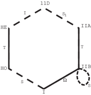
Figure 1: The five ten-dimensional superstring theories are dual to one another. The solid lines denote perturbative dualities, while the dashed ones indicate non-perturbative ones. At strong coupling, both the type $IIA$ and heterotic ${\rm E}_{8}\times{\rm E}_{8}$ strings develop an additional large dimension, a circle ($S_{1}$) and an interval ($I_{1}$) respectively. Therefore, they are both described by an eleven dimensional theory, but this bears no direct relation to strings.

An additional, vexing problem, is that the reduction from ten dimensions to our four-dimensional space time entails a deep lack of predictivity for the low-energy parameters, that depend on the size and shape of the extra dimensions. This fact reflects the absence of a global minimum principle for gravity, similar to those that determine the ground states of a magnet in a weak external field below its Curie temperature or the spontaneous breaking of the electro-weak symmetry in the Standard Model, and represents a stumbling block in all current approaches that aim at deriving our low-energy parameters from String Theory. It has long been hoped that a better understanding of string dynamics would help bypassing this difficulty, but to date no concrete progress has been made on this crucial issue. Thus, ironically, for what we currently understand, String Theory appears to provide a unique answer to the problem of including gravity in the Standard Model, but the four-dimensional remnants of this uniqueness are at least classes of theories. Supersymmetry has again a crucial effect on this problem, since it basically stabilizes the internal geometry, much along the lines of what we have seen for the hierarchy between the electro-weak and Planck scales, but as a result the sizes and shapes (moduli) of the extra dimensions are apparently arbitrary. This is the moduli problem of supersymmetric vacua, a problem indeed, since the resulting low-energy parameters generally depend on the moduli. On the other hand, the breaking of supersymmetry, a necessary ingredient to recover the Standard Model at low energies if we are to describe Fermi and Bose fields of different masses, tends to destabilize the background space time. The end result is that, to date, although we know a number of scenarios to break supersymmetry within String Theory, that we shall briefly review in Section 5, we have little or no control on the resulting space times once quantum fluctuations are taken into account.

The following sections are devoted to some key issues raised by the extension from the Standard Model to String Theory, in an attempt to bring some of the main themes of current research to the attention of the interested reader, while using as starting points basic notions of Electrodynamics, Gravitation and Quantum Mechanics. Our main target will be our colleagues active in Experimental High-Energy Physics, in the spirit of the Moriond Meeting, a very beneficial confrontation between theorists and experimentalists active in Particle Physics today. We hope that this short review will help convey to them the excitement and the difficulties faced by the theorists active in this field.

2 From particles to fields

The basic tenet from which our discussion may well begin is that all matter is apparently made of elementary particles, while our main theme will be to illustrate why this may not be the end of the story. Particles exchange mutual forces, and the Coulomb force between a pair of static point-like charges $q_{1}$ and $q_{2}$,

$$\left|{\bf F}_{C}\right|\sim\frac{|q_{1}\,q_{2}|}{r^{2}}\ ,$$ (2)

with an intensity proportional to their product and inversely proportional to the square of their mutual distance, displays a remarkable similarity with the Newton force between a pair of static point-like masses $m_{1}$ and $m_{2}$,

$$\left|{\bf F}_{N}\right|\sim\frac{|G_{N}\,m_{1}\,m_{2}|}{r^{2}}\ .$$ (3)

Actually, it has long been found more convenient to think of these basic forces in two steps: some “background” charge or mass distribution affects the surrounding space creating a field that, in its turn, can affect other “probe” charges or masses, sufficiently small not to perturb the background significantly. In the first case, the classical dynamics is encoded in the Maxwell equations, that relate the electric field ${\bf E}$ and the magnetic field ${\bf B}$ to electric charges and currents, and as a result both fields satisfy in vacuum wave equations of the type

$$\frac{1}{c^{2}}\ \frac{\partial^{2}\phi}{\partial t^{2}}-\nabla^{2}\phi=0\ .$$ (4)

These entail retardation effects due to the finite speed $c$ with which electromagnetic waves propagate, and, as first recognized by Lorentz and Einstein, provide the route to Special Relativity.

With gravity, the situation is more complicated, since the resulting field equations are highly non linear. According to Einstein’s General Relativity, the gravitational field is a distortion of the space-time geometry that replaces the Minkowski metric $\eta_{\mu\nu}$ with a generic metric tensor $g_{\mu\nu}$, used to compute the distance between two nearby points as

$$ds^{2}=g_{\mu\nu}(x)\,dx^{\mu}\,dx^{\nu}\ .$$ (5)

Material bodies follow universally curved trajectories that reflect the distorted geometries, while the metric $g_{\mu\nu}$ satisfies a set of non-linear wave-like equations where the energy-momentum of matter appears as a source. In fact, the non-linear nature of the resulting dynamics reflects the fact that the gravitational field carries energy, and is therefore bound to act as its own source. These observations extend a familiar fact: in the local uniform gravitational field ${\bf g}$ near the earth ground, Newtonian bodies fall according to

$$m_{i}\,{\bf a}=m_{g}\,{\bf g}\ ,$$ (6)

and the equality of the inertial and gravitational masses $m_{i}$ and $m_{g}$ makes this motion universal. The resulting “equivalence principle” is well reflected in the distorted space-time geometry, that has inevitably a universal effect on test bodies. The modification in (5) can not be the whole story, however, since a mere change of coordinates can do this to some extent, a simple example being provided by the transition to spherical coordinates in three-dimensional Euclidean space, that turns the standard Euclidean metric

$$ds^{2}=dx^{2}+dy^{2}+dz^{2}$$ (7)

into

$$ds^{2}=dr^{2}+r^{2}\,d\theta^{2}+r^{2}\,\sin^{2}\theta\,d\phi^{2}\ .$$ (8)

This simple example reflects a basic ambiguity met when describing the gravitational field via a metric tensor, introduced by the freedom available in the choice of a coordinate system. Strange as it may seem, this is but another, if more complicated, instance of the ambiguity met when describing the Maxwell equations in terms of the potentials ${\bf A}$ and $\Phi$, defined via

$${\bf B}=\nabla\times{\bf A}\ ,\qquad\quad{\bf E}=-\nabla\Phi-\frac{1}{c}\,\frac{\partial{\bf A}}{\partial t}\ ,$$ (9)

a familiar fact of Classical Electrodynamics. This ambiguity, in the form of gauge transformations of parameter $\Lambda$

$${\bf A}\to{\bf A}+\nabla\Lambda\ ,\qquad\quad\Phi\to\Phi-\frac{1}{c}\,\frac{\partial\Lambda}{\partial t}\ ,$$ (10)

does not affect measurable quantities like ${\bf E}$ and ${\bf B}$. A suitable combination of derivatives of $g_{\mu\nu}$, known as the Christoffel connection $\Gamma^{\mu}_{\nu\rho}$, is the proper gravitational analog of the electrodynamic potentials ${\bf A}$ and $\Phi$. Notice the crucial difference: in gravity the potentials are derivatives of the metric field, a fact that has very important consequences, since it essentially determines Eq. 1. In a similar fashion, the gravitational counterparts of the ${\bf E}$ and ${\bf B}$ fields can be built from the Riemann curvature tensor $R^{\mu}{}_{\nu\rho\sigma}$, essentially a curl of the Christoffel connection $\Gamma^{\mu}_{\nu\rho}$, that thus contains second derivatives of $g_{\mu\nu}$. Summarizing, gravity manifests itself as a curvature of the space-time geometry, that falling bodies are bound to experience in their motion.

Notice that Eq. 10 can also be cast in the equivalent form

$${\bf A}\to{\bf A}+\frac{\hbar c}{iq}e^{-\frac{iq\Lambda}{\hbar c}}\,\nabla e^{\frac{iq\Lambda}{\hbar c}}\ ,\qquad\quad\Phi\to\Phi-\frac{\hbar}{iq}\,e^{-\frac{iq\Lambda}{\hbar c}}\frac{\partial\ }{\partial t}\,e^{\frac{iq\Lambda}{\hbar c}}\ ,$$ (11)

a rewriting that has a profound meaning, since it is telling us that in Electrodynamics the effective gauge parameter is a pure phase,

$$\beta=e^{i\frac{q\Lambda}{\hbar c}}\ .$$ (12)

Quantum Mechanics makes this interpretation quite compelling, as can be seen by the following simple reasoning. In Classical Mechanics, the effect of electric and magnetic fields on a particle of charge $q$ is described by the Lorentz force law,

$${\bf F}\ =\ q\left({\bf E}\ +\ \frac{1}{c}\,{\bf v}\times{\bf B}\right)\ ,$$ (13)

while Quantum Mechanics makes use of the Hamiltonian $H$ or of the Lagrangian $L$, from which this force can obtained by differentiation. Thus, $H$ and $L$ are naturally bound to involve the potentials, and so does the non-relativistic Schrödinger equation

$$-\frac{\hbar^{2}}{2m}\,\left(\nabla-\frac{iq}{\hbar c}{\bf A}\right)^{2}\,\psi\ +\ q\,\Phi\,\psi\ =\ i\hbar\,\frac{\partial\psi}{\partial t}\ ,$$ (14)

that maintains its form after a gauge transformation only provided the wave function $\psi$ transforms as

$$\psi\,\to\,e^{\frac{iq}{\hbar c}\Lambda}\,\psi$$ (15)

under the electromagnetic gauge transformation (11), thus leaving the probability density $|\psi|^{2}$ unaffected. Notice that the electromagnetic fields can also be recovered from commutators of the covariant derivatives in (14): for instance

$$\left[\partial_{i}-\frac{iq}{\hbar c}{\bf A}_{i},\partial_{j}-\frac{iq}{\hbar c}{\bf A}_{j}\right]\ =\ -\frac{iq}{\hbar c}\,\left(\partial_{i}{\bf A}_{j}-\partial_{j}{\bf A}_{i}\right)\ =\ -\,\frac{iq}{\hbar c}\,\varepsilon_{ijk}\,{\bf B}_{k}\ .$$ (16)

If Special Relativity is combined with Quantum Mechanics, one is inevitably led to a multi-particle description: quantum energy fluctuations $\Delta E\sim mc^{2}$ can generally turn a particle of mass $m$ into another, and therefore one can not forego the need for a theory of all particles of a given type. Remarkably, the field concept is naturally tailored to describe particles, for instance all the identical photons in nature, and it does so in a relatively simple fashion, via the theory of the harmonic oscillator. A wave equation emerges in fact from the continuum limit of coupled harmonic oscillators, a basic fact nicely reflected by the corresponding normal modes, as can be seen letting

$$\Phi({\bf x},t)\ =\ e^{i\,{\bf k}\cdot{\bf x}}\,f(t)$$ (17)

in Eq. 4. Quantum Mechanics associates to the resulting harmonic oscillators

$$\frac{d^{2}f}{dt^{2}}\ +\ c^{2}\,{\bf k}^{2}\,f\ =\ 0\,,$$ (18)

equally spaced spectra of excitations, that represent identical particles, each characterized by a momentum ${\bf p}=\hbar{\bf k}$, the photons in the present example. The allowed energies are

$$E_{n}({\bf k})\ =\ \hbar\,c\,|{\bf k}|\,\left(n\,+\,\frac{1}{2}\right)\quad(n=0,1,...)\ ,$$ (19)

and the equally spaced spectra allow an identification of the $n$-th excited state with a collection of $n$ photons. Notice the emergence of the zero-point energy $\frac{1}{2}\hbar c\,|\bf{k}|$, a reflection of the uncertainty principle to which we shall return in the following. Let us add that a similar reasoning for fermions would differ in two respects. First, the Pauli principle would only allow $n=0,1$ for each ${\bf k}$, while for the general case of massive fermions with momentum ${\bf p}=\hbar\,{\bf k}$ the allowed energies would be in general

$$E\ =\ \sqrt{c^{2}{\bf p}^{2}+m^{2}c^{4}}\,\left(n-\frac{1}{2}\right)\quad(n=0,1)\ .$$ (20)

Notice the negative zero-point energy, to be compared with the positive zero-point energy for bosons. Incidentally, equal numbers of boson and fermion types degenerate in mass would result in an exactly vanishing zero point energy, a situation realized in models with supersymmetry.

This brings us naturally to a brief discussion of the cosmological constant problem, a wide mismatch between macroscopic and microscopic estimates of the vacuum energy density in our universe. Notice that, in the presence of gravity, an additive contribution to the vacuum energy has sizable effects: energy, just like mass, gives rise to gravitation, and as a result a vacuum energy appears to endow the universe with a corresponding average curvature. Macroscopically, one has a time scale $t_{H}\sim 1/H\sim 10^{17}\,s$, where the Hubble constant $H$ characterizes the expansion rate of our universe, and a simple dimensional argument associates to it an energy density $\rho_{M}\sim\frac{H^{2}\;c^{2}}{G_{N}}$. One can attempt a theoretical estimate of this quantity, following Ya.B. Zel’dovic, taking into account the zero-point energies of the quantum fields that describe the types of particles present in nature. A quantum field, however, even allowing no modes with wavelengths below the Planck length $\ell_{Pl}=\hbar c/E_{Pl}\approx 10^{-33}\,cm$, the Compton wavelength associated to the Planck scale, where as we have seen gravity becomes strong, would naturally contribute via its zero-point fluctuations a Planck energy per Planck volume, or $\rho_{m}\sim E_{Pl}^{4}/(\hbar c)^{3}$. Using Eq. 1 to relate $G_{N}$ to $E_{Pl}$, the ratio between the theoretical estimate of the vacuum energy density and its actual macroscopic value is then

$$\frac{\rho_{M}}{\rho_{m}}\sim\left(\frac{\hbar\;H}{E_{Pl}}\right)^{2}\approx\ 10^{-120}\ .$$ (21)

This is perhaps the most embarrassing failure of contemporary physics, and to many theorists it has the flavor of the blackbody problem, where a similar mismatch led eventually to the formulation of Quantum Mechanics. In a supersymmetric world the complete microscopic estimate would give a vanishing result since, as we have seen, fermions and bosons give opposite contributions to the vacuum energy. Still, with supersymmetry broken at a scale $E_{s}$ in order to allow for realistic mass differences $\delta M\sim E_{s}/c^{2}$ between bosons and fermions, one would essentially recover the previous estimate, but for the replacement of $E_{Pl}$ with the supersymmetry breaking scale $E_{s}$, so that, say, with $E_{s}\sim 1\ TeV$, the ratio in (21) would become about $10^{-88}$, with an improvement of about 30 orders of magnitude. These naive considerations should suffice to motivate the current interest in the search for realistic supersymmetric extensions of the Standard Model with the lowest scale of supersymmetry breaking compatible with current experiments where, accounting also for the contribution of gravity that here we ignored for the sake of simplicity, more sophisticated cancellations can allow to reduce the bound much further. We should stress, however, that no widely accepted proposal exists today, with or without supersymmetry or strings, to resolve this clash between Theoretical Physics and the observed large-scale structure of our universe.

We have thus reviewed how all identical particles of a given type can be associated to the normal modes of a single field. While these are determined by the linear terms in the field equations, the corresponding non-linear terms mediate transformations of one particle species into others. This “micro-Chemistry”, the object of Particle Physics experiments, is regulated by conservation laws, and in fact the basic reaction mechanisms in the Standard Model are induced by proper generalizations of the electromagnetic “minimal substitution” $\nabla\to\nabla-\frac{iq}{\hbar c}A$. The basic idea, as formulated by Yang and Mills in 1954, leads to the non-linear generalization of Electrodynamics that forms the conceptual basis of the Standard Model, and can be motivated in the following simple terms. As we have seen, the electromagnetic gauge transformation

$$U=e^{\frac{iq\Lambda}{\hbar c}}$$ (22)

is determined by a pure phase, that can be regarded as a one-by-one unitary matrix, as needed, say, to describe the effect of a rotation around the $z$ axis of three-dimensional Euclidean space on the complex coordinate $x+iy$. Thus, one might well reconsider the whole issue of gauge invariance for an arbitrary rotation, or more generally for $n\times n$ unitary matrices $U$. What would happen then? First, the electrodynamic potentials would become matrices themselves, while a gauge transformation would act on them as

$$\nabla-\frac{iq}{\hbar c}{\bf A}\ \to\ U\,\left(\nabla-\frac{iq}{\hbar c}{\bf A}\right)\,U^{\dagger}\ .$$ (23)

Moreover, the analogs of the electric and magnetic fields would become non-linear matrix-valued functions of the potentials, as can be seen repeating the derivation in (16) for a matrix potential ${\bf A}_{\mu}$, for which

$$\left[\partial_{\mu}-\frac{iq}{\hbar c}{\bf A}_{\mu},\partial_{\nu}-\frac{iq}{\hbar c}{\bf A}_{\nu}\right]=-\frac{iq}{\hbar c}\,\left(\partial_{\mu}{\bf A}_{\nu}-\partial_{\nu}{\bf A}_{\mu}-\frac{iq}{\hbar c}[A_{\mu},A_{\nu}]\right)=-\,\frac{iq}{\hbar c}\ F_{\mu\nu}.$$ (24)

Notice that the matrix $({\bf A}_{\mu})_{i}{}^{j}$ and the Christoffel symbol $\left(\Gamma_{\mu}\right)_{\nu}{}^{\rho}$ are actually very similar objects, barring from the fact the latter is not an independent field, but a combination of derivatives of $g_{\mu\nu}$.

The resulting Yang-Mills equations

$$[\partial_{\mu}-\frac{iq}{\hbar c}{\bf A}_{\mu},F^{\mu\nu}]=\frac{4\pi}{c}\,J^{\nu}\ ,$$ (25)

to be compared with the more familiar Maxwell equations of Classical Electrodynamics, contain indeed non linear (quadratic and cubic) terms that determine the low-energy mutual interactions of gauge bosons. For instance, the familiar Gauss law of Electrodynamics becomes

$$\nabla\cdot{\bf E}-\frac{iq}{\hbar c}\,({\bf A}\cdot{\bf E}-{\bf E}\cdot{\bf A})=4\pi\rho\ ,$$ (26)

that can not be written in terms of ${\bf E}$ alone. Notice also that the Yang-Mills analogs of ${\bf E}$ and ${\bf B}$ are not gauge invariant. Rather, under a gauge transformation

$$F_{\mu\nu}\to e^{\frac{iq}{\hbar c}\Lambda}\ F_{\mu\nu}\ e^{-\frac{iq}{\hbar c}\Lambda}$$ (27)

so that the actual observables are more complicated in these non-Abelian theories. An example is, for instance, ${\rm tr}(F_{\mu\nu}F^{\mu\nu})$, while a more sophisticated, non-local one, is the Wilson loop

$${\rm tr}\,P\,\exp\left(\frac{iq}{\hbar c}\oint_{\gamma}\,A_{\mu}\,dx^{\mu}\right)\ ,$$ (28)

where $P$ denotes path ordering, the prescription to order the powers of $A_{\mu}$ according to their origin along the path $\gamma$. This non-Abelian generalization of the Aharonov-Bohm phase is of key importance in the problem of quark confinement.

The Standard Model indeed includes fermionic matter, in the form of quark and lepton fields, whose quanta describe three families of (anti)particles, but only the leptons are seen in isolation, so that the non-Abelian ${\rm SU(3)}$ color force is held responsible for the permanent confinement of quarks into neutral composites, the hadrons. The basic interactions of quarks and leptons with the gauge bosons are simple to characterize: as we anticipated, they are determined by minimal substitutions of the type $\nabla\to\nabla-\frac{iq}{\hbar c}{\bf A}$, but some of them violate parity or, in more technical language, are chiral. This fact introduces important constraints due to the possible occurrence of anomalies, quantum violations of classical conservation laws. To give an idea of the difficulties involved, it suffices to consider the Maxwell equations in the presence of a current,

$$\partial_{\mu}\,F^{\mu\nu}=J^{\nu}\ .$$ (29)

Consistency requires that the current be conserved, i.e. that $\partial_{\mu}J^{\mu}=0$, but in the presence of parity violations quantum effects can also violate current conservation, making (29) inconsistent. Remarkably, the fermion content of the Standard Model passes this important test, since all potential anomalies cancel among leptons and quarks.

Figure 2: The first diagram shows a typical contribution to the self-energy of the electron. The virtual particle/anti-particle pair behaves as a small electric dipole, thereby screening the electron charge. Turning to quarks and the strong interaction, in QCD the diagrams of the first kind (where now the wavy line denotes a gluon, rather than a photon) are accompanied by additional ones of the second kind, since the gluons are themselves charged. A direct calculation shows that the anti-screening effect wins, leading to asymptotic freedom.

Another basic feature of the Standard Model is related to the spontaneous breaking of the electro-weak symmetry, responsible for screening the weak force down to very short distances, or equivalently for the masses of the $W^{\pm}$ and $Z$ bosons. This is achieved by the BEH mechanism, whereby the whole of space time hosts a quartet of scalar fields responsible for the screening. Making a vector massive costs a scalar field, that provides the longitudinal polarization of the corresponding waves, so that three scalars are eaten up to build the $W^{+}$, $W^{-}$ and $Z$ bosons, while a fourth massive scalar is left over: this is the Higgs, or more properly the BEH particle, whose discovery would be a landmark event in Particle Physics.

After almost three decades, we are still unable to study the phenomenon of quark confinement in fully satisfactory terms, but we have a host of numerical evidence and simple semi-quantitative arguments to justify our expectations. Thus, in QED (see figure 2) the uncertainty principle fills the actual vacuum with virtual electron-positron pairs, vacuum fluctuations that result in a partial screening of a test charge. This, of course, can also radiate and absorb virtual photons that, however, cannot affect the picture since they are uncharged. On the other hand, the Yang-Mills vacuum (see figure 2) is dramatically affected by the radiation of virtual gauge bosons, that are charged and tend to anti-screen a test charge. The end result of the two competing effects depends on the relative weight of the two contributions, and the color force in QCD is actually dominated by anti-screening. This has an impressive consequence, known as asymptotic freedom: quark interactions become feeble at high energies or short distances, as reflected in the experiments on deep inelastic scattering. A naive reverse extrapolation would then appear to justify intense interactions in the infrared, compatibly with the evident impossibility of finding quarks outside hadronic compounds, but no simple quantitative proof of quark confinement has been attained to date along these lines. On the contrary, even if the weak interactions are also described by a Yang-Mills theory, no subtle infrared physics is expected for them, compatibly with the fact that leptons are commonly seen in isolation: at scales beyond the Compton wavelength of the intermediate bosons, $\ell_{W}\sim 10^{-16}\ cm$, the resulting forces are in fact screened by the BEH mechanism!

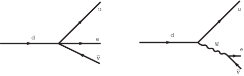
Figure 3: At energies significantly below $100$ GeV, beta decay is well described by a four-fermion interaction. On the other hand, at higher energies the interaction is resolved, or “smeared out”, by the exchange of a $W$ boson.

While more can be said about the Standard Model, we shall content ourselves with these cursory remarks, with an additional comment on the nature of the spontaneous breaking. This ascribes the apparent asymmetry between, say, the short-range weak interactions and the long-range electromagnetic interactions to an asymmetry of the vacuum, much in the same way as the magnetization of a bar can be related to a proper hysteresis. As a result, although hidden, the symmetry is still present, and manifests itself in full power in high-energy virtual processes, making the theory renormalizable like Quantum Electrodynamics is, a crucial result recognized with the Nobel prize to G. ’t Hooft and M. Veltman in 1999. A by-product of the BEH mechanism is a simple relation between the Fermi constant and, say, the $W$ mass $M_{W}$

$$G_{F}\sim\frac{\hbar^{3}\alpha}{c\,M_{W}^{2}}\ ,$$ (30)

with $\alpha$ a dimensionless number of the order of the QED fine-structure constant. This reflects again the fact that the weak forces are completely screened beyond the Compton wavelength of their carriers, $\lambda_{W}\sim\frac{\hbar}{cM_{W}}$, but an equivalent, rather suggestive way of stating this result, is to note that the growth of the effective fine-structure function

$$\alpha_{F}(E)\sim\frac{G_{F}\,E^{2}}{\hbar^{3}c^{3}}\ ,$$ (31)

actually stops at the electro-weak scale $E_{W}\approx\sqrt{\hbar^{3}c^{3}}/\sqrt{G_{F}}$ to leave room to an essentially constant coupling. This transition results from the emergence of new degrees of freedom that effectively smear out the local four-Fermi interaction into QED-like exchange diagrams, as in figure 3.

Given these considerations, it is tempting and natural to try to repeat the argument for gravity, constructing the corresponding dimensionless coupling,

$$\alpha_{N}(E)\sim\frac{G_{N}\,E^{2}}{\hbar\,c^{5}}\ .$$ (32)

The relevant scale is now the Planck scale $E_{Pl}\approx 10^{19}GeV$, but the problem is substantially subtler, since now energy itself is to be spread, and here is where strings come into play. According to figures 4 and 5, a simple, if rather crude, argument to this effect is that if a pair of point masses experiencing a hard gravitational collision are replaced with strings of length $\ell_{s}$, asymptotically only a fraction of their energies is effective in the interaction, so that $\alpha_{N}(E)$ actually saturates to a finite limiting value, $G_{N}\hbar/\ell_{s}^{2}c^{3}$. This simple observation can be taken as the key motivation for strings in this context, and indeed a detailed analysis shows that the ultraviolet problem of gravity is absent in String Theory. A subtler issue is to characterize what values of $\ell_{s}$ one should actually use, although naively the previous argument would lead to identify $\ell_{s}$ with the Planck length $\ell_{Pl}\approx 10^{-33}cm$.

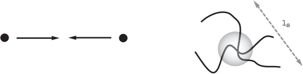
Figure 4: A hard gravitational collision can be softened if point particles are replaced by strings of length $\ell_{s}$. The energy is then spread over their length, while at high energies the effective gravitational coupling $\alpha_{N}(E)=G_{N}E^{2}/\hbar c^{5}$ is replaced by $\alpha_{N}(E)\times((\hbar c/E)/\ell_{s})^{2}$, according to the fraction of the energy effective in the collision.

Figure 5: Replacing point particles with strings, a graviton three-point interaction (left) is “smeared” to such an extent that, in the resulting three-string vertex (right) even no localized interaction point can be found anymore.

3 From fields to strings

This brings us naturally to strings, that clearly come in two varieties, open and closed. It is probably quite familiar that an ordinary vibrating string has an infinity of harmonics, that depend on the boundary conditions at its ends, but whose frequencies are essentially multiples of a fundamental tone. In a similar fashion, a single relativistic string has an infinity of tones, naively related to an infinity of masses according to

$$m^{2}\sim N\,\omega^{2}\ ,\qquad(N\geq 1)$$ (33)

with $N$ an integer, and thus apparently describes an infinity of massive particle species. There is a remarkable surprise, however: the dynamics of strings requires a higher-dimensional Minkowski space and typically turns the previous relation into

$$m^{2}\sim(N-1)\,\omega^{2}\ ,$$ (34)

so that string spectra actually include massless modes, as needed to describe long-range forces. A more detailed analysis would reveal that open strings include massless vectors, while closed strings include massless spin-2 fields. Therefore, not only is one softening the gravitational interactions by spreading mass or energy, but one is also recovering without further ado gauge bosons and gravitons from the string modes.

A closer look would reveal that strings can also describe space-time fermions, with the chiral interactions needed in the Standard Model. Their consistency, however, rests on a new mechanism, discovered by M.B. Green and J.H. Schwarz, that supplements the ordinary anomaly cancellations at work in the Standard Model with the contributions of new types of particles. In their simplest manifestation, these have to do with a two-form field, a peculiar generalization of the electrodynamic potential $A_{\mu}$ bearing an antisymmetric pair of indices, so that $B_{\mu\nu}=-B_{\nu\mu}$. The corresponding field strength, obtained as in Electrodynamics from its curl, is in this case the three-form field $H_{\mu\nu\rho}=\partial_{\mu}B_{\nu\rho}+\partial_{\nu}B_{\rho\mu}+\partial_{\rho}B_{\mu\nu}$. Two-form fields have a very important property: their basic electric sources are strings, just like the basic electric sources in the Maxwell theory are particles. Thus, in retrospect, a $B_{\mu\nu}$ field is a clearcut signature of an underlying string extension. A field of this type is always present in the low-energy spectra of string models, but is absent in the CJS supergravity that, for this reason, as stressed in the Introduction, bears no direct relation to strings.

We have already mentioned that there are apparently several types of string models, all defined in space times with a number of extra dimensions. At present, the only direct way to describe their interactions is via a perturbative expansion. Truly enough, this is essentially the case for the Standard Model as well, but for strings we still lack somehow a way to go systematically beyond perturbation theory. There is a framework, known as String Field Theory, vigorously pursued over the years by a small fraction of the community, and most notably by A. Sen and B. Zwiebach, that is starting to produce interesting information on the string vacuum state, but it is still a bit too early to give a fair assessment of its real potential in this respect. Indeed, even the very concept of a string could well turn out to be provisional, a convenient artifice to describe in one shot an infinity of higher-spin fields, much in the spirit of how a generating function in Mathematics allows one to describe conveniently in one shot an infinity of functions, and in fact String Theory appears in some respect as a BEH-like phase of a theory with higher spins . This is another fascinating, difficult ad deeply related subject, pursued over the years mostly in Russia, and mainly by E. Fradkin and M. Vasiliev.

String Theory allows two types of perturbative expansions. The first is regulated by a dimensionless parameter, $g_{s}$, that takes the place in this context of the fine-structure constants present in the Standard Model, while the second is a low-energy expansion, regulated by the ratio between typical energies and a string scale $M_{s}\sim\hbar/c\,\ell_{s}$ related to the “string size” $\ell_{s}$. In the following we shall use interchangeably the two symbols $\ell_{s}$ and $\alpha^{\prime}=\ell_{s}^{2}$ to characterize the string size. A key result of the seventies, due mainly to J. Scherk, J.H. Schwarz and T. Yoneya, is that in the low-energy limit the string interactions embody both the usual gauge interactions of the Standard Model and the gravitational interactions of General Relativity. Thus, to reiterate, String Theory embodies by necessity long-range electrodynamic and gravitational quanta, with low-energy interactions consistent with the Maxwell (or Yang-Mills) and Einstein equations.

The extra dimensions require that a space-time version of symmetry breaking be at work to recover our four-dimensional world. The resulting framework draws from the original work of Kaluza and Klein, and has developed into the elegant and rich framework of Calabi-Yau compactifications, but some of its key features can be illustrated by a simple example. To this end, let us consider a massless scalar field $\phi$ that satisfies in five dimensions the wave equation

$$\frac{1}{c^{2}}\,\frac{\partial^{2}\phi}{\partial t^{2}}\ -\ \nabla^{2}\phi\ -\ \frac{\partial^{2}\phi}{\partial y^{2}}\ =\ 0\ ,$$ (35)

where the fifth coordinate has been denoted by $y$. Now suppose that $y$ lies on a circle of radius $R$, so that $y\sim y+2\pi R$, or, equivalently, impose periodic boundary conditions in the $y$-direction. One can then expand $\phi$ in terms of a complete set of eigenfunctions of the circle Laplace operator, plane waves with quantized momenta, writing

$$\phi(x,y)=\sum_{n\in\mathbb{Z}}\phi_{n}(x)\,e^{i\,n\,y/R}\ .$$ (36)

Plugging this expansion in the Klein-Gordon equation shows that, from the four-dimensional viewpoint, the mode coefficients $\phi_{n}(x)$ describe independent fields with masses $n/R$, satisfying

$$\frac{1}{c^{2}}\,\frac{\partial^{2}\phi_{n}}{\partial t^{2}}\ -\ \nabla^{2}\phi_{n}\ +\ \frac{n^{2}}{R^{2}}\,\phi=0\ .$$ (37)

At low energies, where the massive modes are frozen, the extra dimension is thus effectively screened and inaccessible, since only quanta of the zero-mode field can be created. Simple as it is, the example suffices to show that the spectrum of massive modes reflects the features of the internal space, in that it depends on the radius $R$. By a slight complication, for instance playing with anti-periodic modes, one could easily see how even the numbers and types of low-lying modes present reflect in general the features of the internal space. This is perhaps the greatest flaw in our current understanding: the four-dimensional manifestations of a given string, and in particular the properties of its light particles, are manifold, since they depend on the size and shape of the extra dimensions. Let us stress that, while in the electro-weak breaking we dispose of a clear minimum principle that drives the choice of a vacuum, no general principle of this type is available in the presence of gravity. Therefore, despite many efforts over the years, we have at present no clearcut way to make a dynamical choice between the available possibilities and, as a result, we are still not in a position to give clearcut string predictions for low-energy parameters. Nonetheless, these possibilities include, rather surprisingly, four-dimensional worlds with gauge and matter configurations along the lines of the Standard Model, although inheriting chiral interactions from higher dimensions would naively appear quite difficult. We may thus be driven to keep an eye on a different and less attractive possibility, as with the old, ill-posed problem, of deriving from first principles the sizes of the Keplerian orbits. As we now understand, these result from accidental initial conditions, and a similar situation for the four-dimensional string vacuum, while clearly rather disturbing, cannot be fairly dismissed at the present time.

Still, in moving to String Theory as the proper framework to extend the Standard Model, it would be reassuring to foresee some sort of uniqueness in the resulting picture, at least in higher dimensions. Remarkably this was achieved, to a large extent, by the mid nineties, and we have now good reasons to believe that all ten-dimensional superstring models are somehow equivalent to one another. The basic equivalences between the four superstring models of oriented closed strings, IIA, IIB, heterotic SO(32) and heterotic ${\rm E}_{8}\times{\rm E}_{8}$, and the type I model of unoriented closed and open strings, usually called string dualities, are summarized in figure 1. The solid links, labeled by $T$ and $\Omega$, can be explicitly established in string perturbation theory, while the additional dashed links rely on non-perturbative arguments that rest on the unique features of the low-energy ten-dimensional supergravity. We can now comment a bit on the labels, beginning with the $T$ duality.

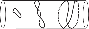
Figure 6: Contrary to point particles, closed strings can wind in a non-trivial way around a compact direction. here we show, from left to right, three examples of closed strings with winding numbers 0, 1 and 2, respectively.

When a particle lives in a circle, the de Broglie wave $e^{\frac{ipx}{\hbar}}$ can be properly periodic only if the momentum is quantized in units of the inverse radius $R$, i.e. if $p=n\hbar/R$. We have already met the field counterpart of this property above, when we have described how a massless five-dimensional field would manifest itself to a four-dimensional observer as an infinite tower of massive fields. A closed string can also be endowed with a center of mass momentum, quantized for the same reason in units of $1/R$, and thus a single string spectrum would appear by necessity to a lower-dimensional observer as a tower of string spectra. However, a closed string can also wrap around the circle an arbitrary number of times, so that in fact a closed string coordinate admits expansions of the type

$$X(\sigma,\tau)=x\ +\ (2\alpha^{\prime})\frac{m}{R}\,\tau\ +\ 2nR\sigma\ +\ \frac{i}{2}\sqrt{2\alpha^{\prime}}\ \sum_{k\neq 0}\left(\frac{\alpha_{k}}{k}\,e^{-i2k(\tau-\sigma)}\ +\ \frac{\tilde{\alpha}_{k}}{k}\,e^{-i2k(\tau+\sigma)}\right)\ ,$$ (38)

where $\tau$ replaces in this context the “proper time” of particle dynamics while $\sigma$ labels the points of the string. Notice that the third term implies that $X(\pi,\tau)=X(0,\tau)+2\pi nR$, as pertains to a closed string winding $n$ times around a circle. The spectrum of the string as seen from the uncompactified dimensions will have the form,

$$M^{2}=\frac{\hbar^{2}}{c^{2}}\left(\frac{m^{2}}{R^{2}}+\frac{n^{2}R^{2}}{\alpha^{\prime}{}^{2}}\right)+\cdots,$$ (39)

where the dots stand for contributions due to the higher frequencies of the string (see e.g. Eq. 33). While the first term in (39) is familiar from ordinary Quantum Mechanics, the second, that as we have seen reflects the possibility of having non-trivial windings, is new and intrinsically “stringy”. Notice that Eq. 39 displays a remarkable symmetry: one cannot distinguish somehow between a string propagating on a circle of radius $R$ and another propagating on a circle with the “dual” radius $\alpha^{\prime}/R\,$! We have actually simplified matters to some extent, since in general $T$-duality affects the fermion spectra of closed strings. Upon circle compactification, it thus maps the two heterotic models and the two type II models into one another, providing two of the solid duality links in figure 1.

The other solid link, labeled by $\Omega$, reflects an additional peculiarity, the simultaneous presence of two sets of modes in a closed string (the “right-moving” $\alpha$ and “left-moving” $\tilde{\alpha}$ modes in Eq. 38). If a symmetry is present between them, as is the case only for the type IIB model, one can use it to combine states, but string consistency conditions require in general that new sectors emerge. As a result, combining in this fashion states of closed strings, one is generally led to introduce open strings as well. This construction, now commonly called an orientifold, was introduced long ago by one of the present authors and was then widely pursued over the years at the University of Rome “Tor Vergata”. It links the type IIB and type I models in the diagram, offering also new perspectives on the issue of string compactification.

The additional, dashed links in figure 1, are harder to describe in simple terms, but can be characterized as analogues, in this context, of the electric-magnetic duality of Maxwell’s Electrodynamics. It is indeed well-known that, in the absence of sources, the electric-magnetic duality transformations ${\bf E}\to{\bf B}$ and ${\bf B}\to-{\bf E}$ are a symmetry of the Maxwell equations

$$\nabla\cdot{\bf E}=0\qquad\nabla\times{\bf E}=-\frac{1}{c}\,\frac{\partial{\bf B}}{\partial t}$$

$$\nabla\cdot{\bf B}=0\qquad\nabla\times{\bf B}=\frac{1}{c}\,\frac{\partial{\bf E}}{\partial t}\ ,$$ (40)

but it is perhaps less appreciated that the symmetry can be extended to the general case, at the expense of turning electric charges and currents into their magnetic counterparts. Whereas these are apparently not present in nature, Yang-Mills theories generically, but not necessarily, predict the existence of heavy magnetic poles, of masses $M\sim M_{W}/\alpha_{e}$, with $\alpha_{e}$ a typical (electric) fine-structure constant. Thus, we might well have failed to see existing magnetic poles, due to their high masses, about 100 times larger than those of the $W$ and $Z$ bosons! Actually, QED could be also formulated in terms of magnetic carriers, but for Quantum Mechanics, that adds an important datum: the resulting magnetic fine-structure constant $\alpha_{m}$ would be enormous, essentially the inverse of the usual electric one. More precisely, magnetic and electric couplings are not independent, but are related by Dirac quantization conditions, so that

$$\alpha_{e}\sim\frac{1}{\alpha_{m}}\ ,$$ (41)

and therefore it is the smallness of $\alpha_{e}$ that favors the usual electric description, where the actual interacting electrons and photons are only mildly different from the corresponding free quanta, on which our intuition of elementary particles rests.

In String Theory, the “electric” coupling is actually determined by the vacuum expectation value of a ubiquitous massless scalar field, the dilaton (closely related to the Brans-Dicke scalar, a natural extension of general relativity), according to

$$g_{s}=e^{\langle\varphi\rangle}\ ,$$ (42)

and at this time we have no direct insight on $g_{s}$, that in general could be space-time dependent. It is thus interesting to play with these $S$ dualities, that indeed fill the missing gaps in figure 1. A surprise is that both the type IIA and the ${\rm E}_{8}\times{\rm E}_{8}$ heterotic models develop at strong coupling an additional dimension, invisible in perturbation theory, but macroscopic if $g_{s}$ is large enough. The emergence of the additional dimension brings into the game the CJS supergravity, the unique supergravity model in eleven dimensions, that however can not be directly related to strings: as we have stressed, it does not contain a $B_{\mu\nu}$ field, although it does contain a three-index field, $A_{\mu\nu\rho}$, related to corresponding higher-dimensional solitonic objects, that we shall briefly return to in the next section, the M2- and M5-branes. This is the puzzling end of the story alluded to in the Introduction: duality transformations of string models, that supposedly describe the microscopic degrees of freedom of our world, link them to a supergravity model with no underlying string. This is indeed, in some respect, like ending up with pions with no clue on the underlying “quarks”! This beautiful picture was contributed in the last decade by many authors, including M. Duff, A. Font, P. Horava, C.M. Hull, L. Ibanez, D. Lust, F. Quevedo, A. Sen, P.K. Townsend, and most notably by E. Witten.

Let us conclude this section by stressing that a duality is a complete equivalence between the spectra of two apparently distinct theories. We have met one example of this phenomenon above, when we have discussed the case of $T$ duality: winding modes find a proper counterpart in momentum modes, and vice versa. Now, in relating the heterotic SO(32) model, say, to the type I string, their two sets of modes have no way to match directly. For instance, a typical open-string coordinate

$$X=x+(2\alpha^{\prime})\frac{m}{R}\,\tau+2nR\sigma+i\sqrt{2\alpha^{\prime}}\ \sum_{k\neq 0}\frac{\alpha_{k}}{k}e^{-ik\tau}\,\cos(k\sigma),$$ (43)

is vastly different from the closed-string expansion met above, since for one matter it involves a single set of modes. How can a correspondence of this type hold? We have already stumbled on the basic principle, when we said that typically Yang-Mills theories also describe magnetic poles. These magnetic poles are examples of solitons, stable localized blobs of energy that provide apparently inequivalent descriptions of wave quanta, to which we now turn.

4 From strings to branes

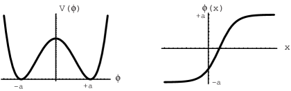
Figure 7: A scalar field theory in $1+1$ dimensions (denoting the scalar field as $\phi(t,x)$), with a potential $V(\phi)=\lambda(\phi^{2}-a^{2})^{2}$ (shown on the left) admits a static, finite energy solution that interpolates between the two vacua $\phi=\pm a$ (shown on the right), known as a “kink”. Its energy or mass is $m^{3}/12\lambda$, where $m$ is the mass of the elementary scalar field. In the perturbative regime, i.e. for small coupling $\lambda$, the kink is therefore very heavy.

A number of field theories admit solitonic solutions, blobs of energy whose shape is stabilized by non-linear couplings. A simple example is provided by the “kink”, that interpolates between the two minima of the potential shown in figure 7. It can be regarded as a model for a wall separating a pair of Curie-Weiss domains in a ferromagnet. Its stability can be argued by noticing that any attempt to deform it, say, to the constant vacuum $\phi=a$ would cost, in one dimension, an energy of the order of $LV(0)$, where $L$ is the size of the region where the field theory lives and $V(0)$ is the height of the potential barrier. For a macroscopic size $L$ this becomes an infinite separation, and the solution is thus stable. Moreover, its energy density, essentially concentrated in the transition region, results in a finite total energy, $E=m^{3}/12\lambda$, where $m$ denotes the mass of the elementary scalar field, defined expanding around one of the minima of the potential, $\phi=\pm a$. This energy defines the mass of the soliton and, as anticipated, blows up in the limit of small coupling $\lambda$. The ‘t Hooft-Polyakov monopole works, in three dimensions, along similar lines: any attempt to destroy it would cost an infinite energy: as is usually said, these objects are topologically stable, and in fact their stability can be ascribed to the conservation of a suitable (topological) charge, that for the monopole is simply its magnetic charge. A further feature of solitons is that their energy is proportional to an inverse power of a coupling constant, as we have seen for the kink. This is simple to understand in general terms: the non-linear nature of the field equations is essential for the stability of solitons, that therefore should disappear in the limit of small coupling!

A localized distribution of energy and/or charge is indeed a modern counterpart of our classical idea of a particle. It is probably familiar that an electron has long been modeled in Classical Electrodynamics, in an admittedly ad hoc fashion, as a spherical shell with a total charge $e$ and a finite radius $a$, associating the resulting electrostatic energy

$$E\sim\frac{e^{2}}{a}$$ (44)

with the electron mass. In a similar fashion, the localized energy distribution of a soliton is naturally identified with a particle, just like an energy distribution localized along a line is naturally identified with an infinite string, while its higher dimensional analogs define generalized branes. Thus, for instance, the “kink” describes a particle in 1+1 dimensions, a string in 1+2 dimensions, where the energy distribution is independent of a spatial coordinate, and a domain wall or two-brane in 1+3 dimensions, where the energy distribution is independent of two spatial coordinates. These are therefore new types of “quanta”, somehow missed by our prescription of reading particle spectra from free wave equations. Amusingly enough, one can argue that the two descriptions of particles are only superficially different, while the whole picture is well fit with Quantum Mechanics. The basic observation is that these energy blobs have typically a spatial extension

$$\Delta\sim\frac{\hbar}{Mc}\ ,$$ (45)

where $M$ denotes a typical mass scale associated to a BEH-like phenomenon, since they basically arise from regions where a transition between vacua takes place, typically of the order of the Compton wavelength (45). In addition, the energy stored in these regions, that determines the mass of the soliton, is

$$M_{sol}\sim\frac{M}{\alpha}\ ,$$ (46)

with $\alpha$ a typical fine-structure constant. At weak coupling (small $\alpha$) we have quantitative means to explore further the phenomenon, but $M_{sol}\gg M$, so that the Compton wavelength of the soliton is well within its size. In other words, in the perturbative region the soliton is a classical object. On the other hand, in the strong-coupling limit (large $\alpha$) the soliton becomes light while its Compton wavelength spreads well beyond its size, so that its inner structure becomes immaterial: we are then back to something very similar in all respects to an ordinary quantum.

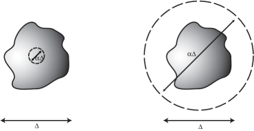
Figure 8: An “artistic” impression of a soliton of size $\Delta$. The dashed circle depicts its Compton wavelength $\lambda_{C}\sim\alpha\Delta$, with $\alpha$ a dimensionless fine-structure constant. The first figure refers to the weak-coupling regime, where $\alpha$ is very small and, as a result, the Compton wavelength $\lambda_{C}$ is much smaller than the soliton size $\Delta$. In this regime, the soliton can be regarded as a classical object. The second figure refers to the strong-coupling regime, where $\alpha$ is very large and, as a result, the Compton wavelength $\lambda_{C}$ is much larger than the soliton size $\Delta$. In this regime, the soliton can be regarded as an ordinary light quantum without any inner substructure.

Solitons are generally interacting objects. For instance, magnetic poles typically experience the magnetic dual of the usual Coulomb force. This is reflected in the fact that, being solutions of non-linear equations, they can not be superposed. In special cases, their mutual forces can happen to cancel, and then, quite surprisingly, the corresponding non-linear field equations allow a superposition of different solutions. This is a typical state of affairs in supersymmetric theories, realized when special inequalities, called “BPS bounds”, are saturated.

The $T$ and $S$ dualities discussed in the previous section can also be seen as maps between ordinary quanta and solitons. The former, simpler case, involves the interchange of momentum excitations with winding modes that, as we have stressed, describe topologically inequivalent closed-string configurations on a circle, while the latter rests on similar operations involving solitons in space time. These, as in the two examples we have sketched in this section, can be spotted from the field equations for the low-energy string modes, but some of their features can be discussed in simple, general terms. To this end, let us begin by rewriting the (1+3)-dimensional Maxwell equations (40) in covariant notation, while extending them to the form

$$\partial_{\mu}\,F^{\mu\nu} = \frac{4\pi}{c}\,J_{e}^{\nu}\ ,$$ (47)

$$\varepsilon^{\mu\nu\rho\sigma}\,\partial_{\nu}\,F_{\rho\sigma} = \frac{4\pi}{c}\,{J}_{m}^{\nu}\ ,$$ (48)

where, in addition to the more familiar electric sources $J_{e}$, we have also introduced magnetic sources $J_{m}$, that affect the Faraday-Neumann-Lenz induction law and the magnetic Gauss law. Notice how a current $J_{e}^{\mu}$ is naturally borne by particles, with $J_{e}^{\mu}\sim q\,u^{\mu}$ in terms of their charge and four-velocity. In $D>4$, however, the $\varepsilon$ tensor carries $D$ indices, and consequently $J_{m}$ carries in general $D-3$ indices, while its sources are extended objects defined via $D-4$ Lorentz indices. Thus, a magnetic pole is a particle in four dimensions as a result of a mere accident. In six dimensions, for instance, the magnetic equations would become

$$\varepsilon^{\mu\nu\rho\sigma\tau\lambda}\,\partial_{\sigma}\,F_{\tau\lambda}=\frac{4\pi}{c}\,\tilde{J}_{m}^{\mu\nu\rho}\ ,$$ (49)

so that by the previous reasoning a magnetic pole would bear a pair of indices, as pertains to a surface. In other words, it would be a two-brane. The argument can be repeated for a general class of tensor gauge fields, $B_{\mu_{1}\cdots\mu_{p+1}}$, in $D$ dimensions: their electric sources are $p$-branes, while the corresponding magnetic sources are $(D-4-p)$-branes. These tensor gauge fields are typically part of low-energy string spectra, while the corresponding “electric” and “magnetic” poles show up as solutions of the complete low-energy equations for the string modes. As we have seen, they define new types of “quanta” that are to be taken into account: in fact, “branes” of this type are the missing states alluded to at the end of the previous section!

As stressed by J. Polchinski, a peculiarity of String Theory makes some of the “branes” lighter than others in the small-coupling limit and, at the same, simpler to study. The first feature is due to a string modification of Eq. 46, that for these “D-branes” happens to depend on $\sqrt{\alpha}\sim g_{s}$, rather than on $\alpha$, as is usually the case for ordinary solitons. The second feature is related to the possibility of defining String Theory in the presence of D-branes via a simple change of boundary conditions at the string ends. In other words, D-branes absorb and radiate strings. In analogy with ordinary particles, D-branes can be characterized by a tension (mass per unit volume) and a charge, that defines their coupling to suitable tensor gauge fields. While their dynamics is prohibitively complicated, in the small coupling limit they are just rigid walls, and so one is effectively studying some sort of Casimir effect induced by their presence. The idea is hardly new: for instance, the familiar Lamb shift of QED is essentially a Casimir effect induced by the atom. What is new and surprising in this case, however, is that the perturbation theory around D-branes can be studied in one shot for the whole string spectrum. In other words, for an important class of phenomena that can be associated to D-branes, a macroscopic analysis of the corresponding field configurations can be surprisingly accompanied by a microscopic analysis of their string fluctuations. This is what makes D-branes far simpler than other string solitons, for instance the M5-brane, on which we have very little control at this time. The mixing of left and right closed-string modes met in the discussion of orientifolds in the context of string dualities can also be given a space-time interpretation along these lines: it is effected by apparently non-dynamical “ends of the world”, usually called O-planes. There is also an interesting possibility, well realized in perturbative open-string constructions: while branes, being physical objects, are bound to have a positive tension, one can allow different types of O-planes, with both negative and positive tension. While the former are typical ingredients of supersymmetric vacua, the latter can induce interesting mechanisms of supersymmetry breaking that we shall mention briefly in the next section.

5 Some applications

The presence of branes in String Theory provides new perspectives on a number of issues of crucial conceptual and practical import. In this section we comment briefly on some of them, beginning with the amusing possibility that our universe be associated to a collection of branes, and then moving on to brief discussions of black hole entropy and color-flux strings.

5.1 Particle Physics on branes?

One is now confronted with a fully novel situation: as these “branes” are extended objects, one is naturally led to investigate the physics of their interior or, in more pictorial terms, the physics as seen by an observer living on them. To this end, it is necessary to study their small oscillations, that define the light fields or, from what we said in the previous sections, the light species of particles seen by the observer. These will definitely include the scalars that describe small displacements of the “branes” from their equilibrium positions, and possibly additional light fermionic modes. A surprising feature of D-branes is that their low-energy spectra also include gauge fields. Both scalars and gauge fields arise from the fact that open strings end on D-branes (seen from the brane, their intersections are point-like), and are in fact associated to string fluctuations transversal or longitudinal to the branes, respectively. In addition, when several branes coincide non-Abelian gauge symmetries arise, as summarized in figure 9. In equivalent terms, the mutual displacement of branes provides a geometric perspective on the BEH mechanism. Moreover, the low-energy dynamics of gauge fields on a $Dp$-brane is precisely of the Yang-Mills type, but at higher energies interesting stringy corrections come into play. While a proper characterization of the general case is still an open problem, in the Abelian case of a single D-brane, and in the limit of slowly varying electric and magnetic fields, String Theory recovers a beautiful action proposed in the 1930’s by Born and Infeld to solve the singularity problem of a classical point-like electric charge, as originally shown by E. Fradkin and A. Tseytlin. Let us explain briefly this point. Whereas in the usual Maxwell formulation the resulting Coulomb field

$${\bf E}=\frac{q}{r^{2}}\ {\bf\hat{r}}\ ,$$ (50)

where ${\bf\hat{r}}$ denotes the unit radial vector, leads to an infinite energy, in String Theory the Maxwell action for the static case is modified, and takes the form

$$-\frac{1}{2}\,{\bf E}^{2}\to\frac{1}{2\pi\alpha^{\prime}}\ \sqrt{1-2\pi\alpha^{\prime}\,{\bf E}^{2}}$$ (51)

so that Eq. (50) is turned into

$${\bf E}=\frac{q}{\sqrt{r^{4}+(2\pi\alpha^{\prime})^{2}}}\,{\bf\hat{r}}\ .$$ (52)

As a result, the electric field strength saturates to $\frac{q}{2\pi\alpha^{\prime}}$, much in the same way as the speed of a relativistic particle in a uniform field saturates to the speed of light $c$, an analogy first stressed in this context by C. Bachas. Thus, once more String Theory appears to regulate divergences, as we have already seen in connection with the ultraviolet problem of gravity.

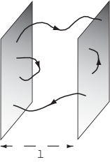
Figure 9: A system consisting of two parallel D-branes, to which oriented open strings can attach in four different ways. The masses of the gauge fields associated to the four types of open strings are proportional to the shortest distances between the branes they connect. When the mutual distance $l$ between the branes is not zero, one is thus describing two massless gauge fields, with a corresponding unbroken $U(1)\times U(1)$ symmetry, and two additional massive $W$-like fields. On the other hand, when $l\rightarrow 0$ the two $W$-like fields become massless as well, while the gauge symmetry enhances to $U(2)$. In this geometric setting for the BEH mechanism, the Higgs scalar describes the fluctuations of the branes relative to one another, while its vacuum value defines their relative distance $l$.

Summarizing, the world volume of a collection of D$p$-branes is by construction a $(p+1)$-dimensional space that contains in principle the right types of light fields to describe the particles of the Standard Model. This observation has changed our whole perspective on the Kaluza-Klein scenario, is at the heart of current attempts to model our universe as a collection of intersecting D-branes, and brings about a novelty that we would like to comment briefly upon. The issue at stake is, again, the apparently unnatural hierarchy between the electro-weak and Planck scales, on which this scenario offers a new geometric perspective, since in a “brane world” gauge and matter interactions are confined to the branes, while gravity spreads in the whole ambient space. One can thus provide a different explanation for the weakness of gravity: most of its Faraday lines spread in the internal space, and are thus simply “lost” for a brane observer. This is the essence of a proposal made by I. Antoniadis, N. Arkani-Ahmed, S. Dimopoulos and G. Dvali, that has stimulated a lot of activity in the community over the last few years. For instance, with $n$ extra circles of radius $R$ one would find that a $(4+n)$-dimensional Newton constant $G_{4+n}$ for bulk gravity induces for two point-like masses on the brane an effective Newton constant $1/G_{4}\sim R^{n}/G_{4+n}$. This result can be obtained adding the contributions of the extra circles or, more simply, purely on dimensional grounds. Playing with the size $R$, one can start with $G_{4+n}\sim\left(1/TeV\right)^{2+n}$ and end up with the conventional $G_{4}\sim 1/(10^{19}GeV)^{2}$, if $R\sim 10^{32/n}\times 10^{-4}fm$, so that if $n\geq 2$ the resulting scenario is not obviously excluded. The phenomenon would manifest itself as a striking change in the power law for the Newton force (3), that for $r<R$ would behave like $1/r^{2+n}$, a dramatic effect indeed, currently investigated by a number of experimental groups at scales somewhat below the millimeter. In a similar fashion, one can also conceive scenarios where the string size $\ell_{s}$ is also far beyond the Planck length, but a closer inspection shows that in all cases the original hierarchy problem has been somehow rephrased in geometrical, although possibly milder, terms: all directions parallel to the world brane should be far below the millimeter, at least ${\cal O}(10^{-16}\ cm)$, if no new phenomena are to be present in the well-explored gauge interactions of the Standard Model at accessible energies, so that a new hierarchy emerges between longitudinal and transverse directions. The literature also contains interesting extensions of this scenario with infinitely extended curved internal dimensions, where gravity can nonetheless be localized on branes, but this simpler case should suffice to give a flavor of the potential role of branes in this context.

It is also possible to complicate slightly this picture to allow for the breaking of supersymmetry. To date, we have only one way to introduce supersymmetry breaking in closed strings working at the level of the full String Theory, as opposed to its low-energy modes: Bose and Fermi fields can be given different harmonic expansions in extra dimensions. For instance, referring to the case of Section 3, if along an additional circle Bose fields are periodic while Fermi fields are anti periodic, the former inherit the masses $k/R$, while the letter are lifted to $(k+1/2)/R$, with supersymmetry broken at a scale $\Delta M\sim 1/R$. This is the Scherk-Schwarz mechanism, first fully realized in models of oriented closed strings by S. Ferrara, K. Kounnas, M. Porrati and F. Zwirner, following a previous analysis of R. Rohm. Branes and their open strings, however, allow new possibilities, known in the literature, respectively, as “brane supersymmetry” and “brane supersymmetry breaking”, that we would like to briefly comment upon. Of course, the mere presence of branes, extended objects of various dimensions, breaks some space-time symmetries, and in fact one can show that a single brane breaks at least half of the supersymmetries of the vacuum, but more can be done by suitable combinations of them. Thus, the first mechanism follows from the freedom to use, in the previous construction, directions parallel or transverse to the “brane world” to separate Fermi and Bose momenta. While momenta along parallel directions reproduce the previous setting, orthogonal ones in principle can not separate brane modes. However, a closer inspection reveals that this is only true for the low-lying excitations, while the massive ones, affected by the breaking, feed it via radiative corrections to the low-lying modes, giving rise a gravitational analogue of the “see-saw” mechanism, with $\Delta M\sim\sqrt{G_{N}}/R^{2}$.

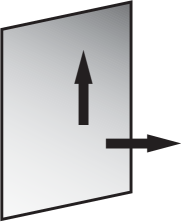
Figure 10: Brane supersymmetry and the gravitational see-saw. If the momenta of Bose and Fermi brane fields are separated along a direction orthogonal to the D-brane, only the massive brane excitations feel the effect, that is then transmitted via radiative corrections to the low-lying excitations, relevant for the Standard Model physics.

Finally, the second mechanism can induce supersymmetry breaking in our world radiatively from other non-supersymmetric branes, with the interesting possibility of attaining a low vacuum energy in the observable world.

By and large, however, one is again led to a puzzling end: a sort of “brane chemistry” allows one to concoct an observable world out of these ingredients, much in the spirit that associates chemical compounds to the basic elements of the Periodic Table, and eventually to electrons and nuclei. However, the problem alluded to in the previous Sections is still with us: we have presently no plausible way of selecting a preferred configuration to connect String Theory to our low-energy world, although one can well construct striking realizations of the Standard Model on intersecting branes, as first shown by the string groups at the Universidad Autonoma de Madrid and at the Humboldt University in Berlin.

Figure 11: The world as a collection of interacting branes. Amusingly, we have come all this way from our matter seen as a collection of point particles, recovering at large scales something quite reminiscent of our starting point.

5.2 Can strings explain Black Hole Thermodynamics?

As we have stressed, D-branes can be given a macroscopic description as solutions of the non-linear field equations for the light string modes, and at the same time a microscopic description as emitters and absorbers of open strings. If for a black hole both descriptions were available, one would be naturally led to regard the open string degrees of freedom as its own excitations. This appears to provide a new perspective on a famous result of S. Hawking, that associates to the formation of a black hole a blackbody spectrum of radiation at a characteristic temperature $T_{H}$. Since, as originally stressed by J. Bekenstein, the resulting conditions for the mass variation of the hole have the flavor of Thermodynamics, D-branes offer the possibility of associating to this Thermodynamics a corresponding Statistical Mechanics, the relevant microstates being their own excitations.

In the presence of a static isotropic source of mass $M$ at the origin, the Minkowski line element is deformed to

$$ds^{2}=\left(1-\frac{2G_{N}M}{r\,c^{2}}\right)c^{2}dt^{2}-\left(1-\frac{2G_{N}M}{r\,c^{2}}\right)^{-1}dr^{2}-r^{2}d\Omega^{2}.$$ (53)

This expression holds outside the source, while the special value of the radial coordinate $r_{h}=2G_{N}Mc^{-2}$ corresponds to the event horizon, that can be characterized as the minimum sphere centered at the origin that is accessible to a far-away observer. For most objects $r_{h}$ lies deep inside the source itself (e.g. for the sun $r_{h}\approx 3\,Km$, to be compared with the solar radius $R\approx 10^{6}\,Km$), where Eq. 53 is not valid anymore, but one can conceive a source whose radius is inferior to $r_{h}$, and this is called a black hole: according to classical General Relativity, any object coming from outside and crossing the horizon is trapped inside it forever. Over the past decade, astrophysical observations have given strong, if indirect, clues that black holes are ubiquitous in our universe.

As anticipated, however, Hawking found that black holes are not really black if Quantum Mechanics is properly taken into account. Rather, quantizing a Field Theory in a background containing a black hole, he showed that to an external observer the hole appears to radiate as a black body with temperature

$$T_{H}\ =\ \frac{c^{3}\,\hbar}{8\pi k_{B}G_{N}M}\ ,$$ (54)

where $k_{B}$ denotes Boltzmann’s constant. This amazing phenomenon that can be made plausible by noting that a virtual particle-antiparticle pair popping up in the neighborhood of the horizon can have such a dynamics that one of the two crosses the horizon, while the other, forced by energy conservation to materialize as a real particle, will do so absorbing and carrying away part of the gravitational energy of the black hole. In analogy with the second law of Thermodynamics, given the temperature $T_{H}$ one can associate to a black hole an entropy

$$\frac{1}{k_{B}}\;S_{H}\ =\ \frac{4\pi G_{N}M^{2}}{c\hbar}\ =\ \frac{1}{4}A_{H}\,\ell_{Pl}^{-2}\ ,$$ (55)

where $A_{H}$ is the area of the horizon and $\ell_{Pl}$ is the Planck length $\ell_{Pl}=\sqrt{G_{N}\hbar/c^{3}}\approx\ 10^{-33}\,cm$, that we have repeatedly met in the previous sections. This expression, known as the Bekenstein-Hawking formula, reflects a universal behavior: the entropy of any black hole is one quarter of the area of its horizon in Planck units.

Several questions arise, that have long puzzled many experts:

• As anything crossing the horizon disappears leaving only thermal radiation behind, the S-matrix of a system containing a black hole seems not unitary anymore, thus violating a basic tenet of Quantum Mechanics. This is known as the information paradox.

• Entropy is normally a measure of the degeneracy of microstates $\Sigma$ in some underlying microscopic description of a physical system, determined by Boltzmann’s formula,

  $$S=k_{B}\,\log\Sigma\ .$$ (56)

  Since the entropy (55) of a black hole is naturally a huge number, how can one exhibit such a wealth of microstates?

• Eq. 54 clearly shows that the more mass is radiated away from the black hole, the hotter this becomes. What is then the endpoint of black hole evaporation?

Within String Theory there is a class of black holes where these problems can be conveniently addressed, the so-called extremal black holes, that correspond to BPS objects in this context. The simplest available example is provided by a source that also carries an electric charge $Q$. The coupled Maxwell-Einstein equations would give in this case the standard Coulomb potential for the electric field, together with the modified line element $(G_{N}M^{2}>Q^{2})$

$$ds^{2}=\left(1-\frac{2G_{N}M}{r\,c^{2}}+\frac{G_{N}Q^{2}}{r^{2}\,c^{4}}\right)dt^{2}-\left(1-\frac{2G_{N}M}{r\,c^{2}}+\frac{G_{N}Q^{2}}{r^{2}\,c^{4}}\right)^{-1}dr^{2}-r^{2}d\Omega^{2},$$ (57)

that generalizes Eq. 53. Notice that the additional terms in (57) have a nice intuitive meaning: $Q^{2}/2r$ is the electrostatic energy introduced by the charge in the region beyond $r$, and this contribution gives rise to a repulsive gravitational effect. The event horizon, defined again as the smallest sphere surrounding the hole that is accessible to a far-away observer, would now be

$$r_{H}=c^{-2}\left(G_{N}M+\sqrt{(G_{N}M)^{2}-G_{N}Q^{2}}\right).$$ (58)

A source with a radius smaller than $r_{H}$ would be a Reissner-Nordstrom black hole, with temperature and entropy given by

$$T_{H} = \frac{c^{3}\hbar\sqrt{(G_{N}M)^{2}-G_{N}Q^{2}}}{2\pi k_{B}(G_{N}M+\sqrt{(G_{N}M)^{2}-G_{N}Q^{2}}\,)^{2}},$$

$$\frac{S_{H}}{k_{B}} = \frac{\pi}{c\hbar G_{N}}(G_{N}M+\sqrt{(G_{N}M)^{2}-G_{N}Q^{2}}\,)^{2}=\frac{1}{4}A_{H}\,l_{p}^{-2}.$$ (59)

For a given value of $Q$, if $M\rightarrow Q/\sqrt{G_{N}}$ the temperature vanishes, so that the black hole behaves somehow in this limiting (BPS) case as if it were an elementary particle. Such a black hole is called extremal: its mass is tuned so that the tendency to gravitational collapse is precisely balanced by the electrostatic repulsion. This limiting case entails a manifestation of the phenomenon alluded to in Section 4: although the Maxwell-Einstein equations are highly non linear, one can actually superpose these extremal solutions.

Extremal black holes of this type can be described in String Theory in relatively simple terms. One of the simplest configurations involves the type IIB string theory compactified on a 5-dimensional torus, together with a D5-brane and a D1-brane wrapped $n_{5}$ and $n_{1}$ times respectively around the torus. This BPS configuration is characterized by two topological numbers, $n_{1}$ and $n_{5}$, but one needs a slight complication of it since, being the only BPS state with these charges, it leads to a vanishing entropy, consistently with Eq. 59. However, suitable excitations, involving open strings ending on the D-branes and wrapping in various ways around the torus, are also BPS and can be characterized by a single additional quantum number, $n_{e}$. Many open string configurations now correspond to a given value of $n_{e}$, and counting them one can obtain a microscopic estimate of the entropy. One can then turn to IIB supergravity on the 5-torus, constructing a BPS solution of its field equations that involves the three charges mentioned above, to calculate its event horizon, its temperature and finally to obtain the corresponding macroscopic estimate of the entropy. The exact agreement between the two estimates is then striking. Since this original example was discussed by A. Strominger and C. Vafa, many other black hole configurations were studied, while the analysis was successfully extended to nearly extremal ones. These results, however, rely heavily on supersymmetry, and serious difficulties are met in attempts to extend them to non-supersymmetric black holes.

The analysis of nearly extremal black holes also appears to provide a clue on the information paradox. Studying a configuration slightly away from extremality, it was indeed found that Hawking radiation can be associated to the annihilation of pairs of open strings, each ending on a D-brane, that give rise to open strings remaining on the brane and to closed strings leaving it. The resulting radiation turns out to be exactly thermal, while temperature and radiation rate are in perfect agreement with a Hawking-like calculation. Almost by construction, this process is unitary, and so the information that seemed lost appears to be left in the D-branes.

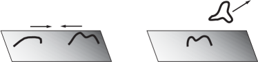
Figure 12: The D-brane picture of Hawking radiation. A pair of open strings collide, giving rise to a closed string that leaves the brane. As a result, Hawking radiation reaches the bulk via the emission of closed strings.

5.3 AdS/CFT: strings for QCD mesons, or is the universe a hologram?

In the previous section we saw that the entropy of a black hole is proportional to the area of its horizon. This is remarkable, since one can argue that black holes maximize the entropy. Indeed, assume for a moment that one managed to construct a physical system in a given volume $V$ with a mass $M-\delta M$ slightly inferior to that of a black hole whose horizon spans the surface surrounding $V$, but with an entropy $S+\delta S$ slightly larger than that of the black hole. Throwing in a bit matter would then create a black hole while simultaneously lowering the entropy, thereby violating the fundamental law of Thermodynamics. This observation led ’t Hooft to propose the Holographic Principle: in a complete theory of quantum gravity, it should be possible to describe the physics of a certain region of spacetime in terms of degrees of freedom living on the surface surrounding it, while the information stored should be limited to roughly one bit per Planck area unit.

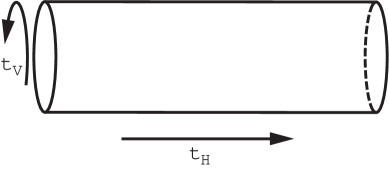
Figure 13: A surprising equivalence in String Theory. An annulus diagram can be regarded as a loop diagram for open strings (with vertical time $t_{V}$), or equivalently as a closed string tree diagram (with horizontal time $t_{H}$).

Over the past few years, concrete realizations of the Holographic principle have been constructed, most dramatically in the context of the so-called AdS/CFT correspondence. In its simplest form, this arises if the type IIB string theory is defined in a ten-dimensional space-time with the topology of a five-dimensional sphere ($S^{5}$) times a five-dimensional anti-de Sitter space ($AdS_{5}$), a non-compact manifold whose boundary can be identified with four-dimensional Minkowski space. This geometry describes the region around the horizon for a stack of $n$ D3-branes, that in the large-$n$ limit actually invades the whole of space time. On the one hand there are therefore D-branes, that as we have seen host a Yang-Mills theory, while on the other there is a corresponding string background, and J. Maldacena conjectured that the resulting string theory (which includes gravity) in the bulk of $AdS_{5}$ is exactly equivalent (dual) to an ${\cal N}=4$ ${\rm U}(n)$ super Yang-Mills theory in its border, the four dimensional Minkowski space. This remarkable correspondence actually reflects a number of unusual equivalences between string amplitudes: for instance, as shown in figure 13, a one-loop diagram for open strings, obtained widening an ordinary field theory loop into an annulus, can alternatively be regarded as a tree-level diagram for closed strings. In other words, the distinction between closed and open strings, and thus between gravity and gauge fields, is somewhat blurred in String Theory. The conjecture was particularly well tested in the regime where the size of the strings is very small compared to the radii of $AdS_{5}$ and $S^{5}$ and where the string coupling constant is also small, so that the string theory is well described by classical supergravity. In the dual picture, this corresponds to the ${\rm U}(n)$ Yang-Mills theory in the limit where both $n$ and the ’t Hooft coupling $g^{2}_{YM}n$ are large, i.e. in its deep quantum mechanical regime. Still, some quantities protected by supersymmetry match mirably in the two descriptions, confirming this surprising correspondence between theories defined in different space-time dimensions. Tests at intermediate regimes are much harder and are still largely lacking, but no contradictions have emerged so far. Gravity would this way ideally provide a tool to study quark confinement, but with a new ingredient: the color flux tubes penetrate an additional dimension of space time.

We have thus come to a full circle somehow. The string idea originated from attempts made in the sixties to model the strong interaction amongst mesons via narrow flux tubes, that culminated in the famous work of G. Veneziano. With the advent of QCD, this picture was abandoned, since the flux tubes were regarded as a manifestation of QCD itself, while strings were proposed, as we have seen, as a tool to attain a finite quantum gravity. However, many people kept looking for a string-like description of the color flux-tubes, and with the advent of the AdS/CFT correspondence this was indeed realized to some extent, albeit once more in a supersymmetric setting that is free of many intricacies of QCD. Again, difficulties of various types are met when one tries to proceed away from supersymmetry to come closer to our real confining low-energy world.

References

References

-
[1]
Some recent books on the Standard Model:
F. Mandl and G. Shaw, “Quantum Field Theory,” Chichester, UK: Wiley, 1984;
M. E. Peskin and D. V. Schroeder, “An Introduction To Quantum Field Theory,” Reading: Addison-Wesley, 1995;
S. Weinberg, “The Quantum Theory of Fields”, Cambridge, UK: Cambridge Univ. Press, 1995. -
[2]
Two books on General Relativity:
W. Weinberg, “Gravitation and Cosmology,” New York, USA: John Wiley & Sons, 1972;
R. M. Wald, “General Relativity,” Chicago, Usa: Univ. Pr., 1984. -
[3]
A review on the ultraviolet problem of quantum gravity:
E. Alvarez, “Quantum Gravity: A Pedagogical Introduction To Some Recent Results,” Rev. Mod. Phys. 61 (1989) 561. -
[4]
Two recent reviews of the BEH mechanism, with
historical remarks:
R. Brout, “A brief course in spontaneous symmetry breaking. I: The paleolitic age,” arXiv:hep-th/0203096;
F. Englert, “A brief course in spontaneous symmetry breaking. II: Modern times: The BEH mechanism,” arXiv:hep-th/0203097. -
[5]
Some technical books on String Theory:
M. B. Green, J. H. Schwarz and E. Witten, “Superstring Theory,” 2 vols., Cambridge, UK: Cambridge Univ. Pr., 1987;
J. Polchinski, “String Theory,” 2 vols., Cambridge, UK: Univ. Pr., 1998;
E. Kiritsis, “Introduction to superstring theory,” arXiv:hep-th/9709062;
D. Lüst and S. Theisen, “Lectures On String Theory,” Lect. Notes Phys. 346 (1989) 1. -
[6]
Some important old reviews on String theory:
“Dual Theory”, ed. M. Jacob, Amsterdam, Netherlands: North-Holland, 1974;
J. Scherk, “An Introduction To The Theory Of Dual Models And Strings,” Rev. Mod. Phys. 47 (1975) 123. -
[7]
A popular book on String Theory:
B.R. Greene, “The Elegant Universe”, New York, USA:W.W. Norton & Co, 1999. -
[8]
A recent review on canonical quantum gravity:
C. Rovelli, “The century of the incomplete revolution: Searching for general relativistic quantum field theory,” J. Math. Phys. 41 (2000) 3776 [arXiv:hep-th/9910131]. -
[9]
Some reviews on the cosmological constant problem:
S. Weinberg, “The Cosmological Constant Problem,” Rev. Mod. Phys. 61 (1989) 1;
E. Witten, “The cosmological constant from the viewpoint of string theory,” arXiv:hep-ph/0002297;
S. M. Carroll, “The cosmological constant,” Living Rev. Rel. 4 (2001) 1 [arXiv:astro-ph/0004075]. -
[10]
Two reviews on open strings and their applications:
E. Dudas, “Theory and phenomenology of type I strings and M-theory,” Class. Quant. Grav. 17 (2000) R41 [arXiv:hep-ph/0006190];
C. Angelantonj and A. Sagnotti, “Open strings,” arXiv:hep-th/0204089. -
[11]
Some books and reviews on Field Theory
solitons:
R. Rajaraman, “Solitons And Instantons”, Amsterdam, Netherlands: North-Holland, 1982;
S. Coleman, “Aspects Of Symmetry”, Cambridge, UK: Cambridge Univ. Press, 1985;
G. ‘t Hooft, “Monopoles, instantons and confinement,” arXiv:hep-th/0010225. -
[12]
A review on string solitons:
M. J. Duff, R. R. Khuri and J. X. Lu, Phys. Rept. 259 (1995) 213 [arXiv:hep-th/9412184]. -
[13]
Some reviews on D-branes and their applications:
J. Polchinski, S. Chaudhuri and C. V. Johnson, “Notes on D-Branes,” arXiv:hep-th/9602052;
C. P. Bachas, “Lectures on D-branes,” arXiv:hep-th/9806199;
C. V. Johnson, “D-brane primer,” arXiv:hep-th/0007170. -
[14]
A less technical review on D-branes:
A. Sevrin, “From strings to branes: a primer” in “Les Arcs 2000, Electroweak interactions and unified theories”. -
[15]
Some reviews on duality relations:
D. I. Olive, “Exact electromagnetic duality,” Nucl. Phys. Proc. Suppl. 45A, 88 (1996) [Nucl. Phys. Proc. Suppl. 46, 1 (1996)] [arXiv:hep-th/9508089];
M. J. Duff, “M theory (the theory formerly known as strings),” Int. J. Mod. Phys. A 11, 5623 (1996) [arXiv:hep-th/9608117];
A. Sen, “Unification of string dualities,” Nucl. Phys. Proc. Suppl. 58 (1997) 5 [arXiv:hep-th/9609176];
P. K. Townsend, “Four lectures on M-theory,” arXiv:hep-th/9612121. -
[16]
Some reviews on the AdS/CFT correspondence:
E. Witten, “New perspectives in the quest for unification,” arXiv:hep-ph/9812208;
O. Aharony, S. S. Gubser, J. M. Maldacena, H. Ooguri and Y. Oz, “Large N field theories, string theory and gravity,” Phys. Rept. 323 (2000) 183 [arXiv:hep-th/9905111];
M. Bianchi, “(Non-)perturbative tests of the AdS/CFT correspondence,” Nucl. Phys. Proc. Suppl. 102 (2001) 56 [arXiv:hep-th/0103112]. -
[17]
Some reviews on
black holes in String Theory:
J. M. Maldacena, “Black holes in string theory,” arXiv:hep-th/9607235;
C. Callan, “Black holes in string theories: some surprising new developments,” in “Les Arcs 1997, Electroweak interactions and unified theories”, 185;
J. R. David, G. Mandal and S. R. Wadia, “Microscopic formulation of black holes in string theory,” arXiv:hep-th/0203048. -
[18]
A recent review on the holographic principle:
R. Bousso, “The holographic principle,” arXiv:hep-th/0203101. -
[19]
Some reviews on heterotic-string phenomenology:
K. R. Dienes, “String Theory and the Path to Unification: A Review of Recent Developments,” Phys. Rept. 287 (1997) 447 [arXiv:hep-th/9602045];
F. Quevedo, “Lectures on superstring phenomenology,” arXiv:hep-th/9603074. -
[20]
Some reviews on large extra dimensions and
open strings:
J. D. Lykken, “String model building in the age of D-branes,” Nucl. Phys. Proc. Suppl. 52A (1997) 271 [arXiv:hep-th/9607144];
L. E. Ibanez, “New perspectives in string phenomenology from dualities,” arXiv:hep-ph/9804236;
L. E. Ibanez, “The second string (phenomenology) revolution,” Class. Quant. Grav. 17 (2000) 1117 [arXiv:hep-ph/9911499];
I. Antoniadis, “String and D-brane physics at low energy,” arXiv:hep-th/0102202;
I. Antoniadis and K. Benakli, “Large dimensions and string physics in future colliders,” Int. J. Mod. Phys. A 15 (2000) 4237; [arXiv:hep-ph/0007226]
C. P. Bachas, “Scales of string theory,” Class. Quant. Grav. 17 (2000) 951 [arXiv:hep-th/0001093];
L. E. Ibanez, “Standard model engineering with intersecting branes,” arXiv:hep-ph/0109082;
R. Blumenhagen, B. Kors, D. Lust and T. Ott, “Intersecting brane worlds on tori and orbifolds,” arXiv:hep-th/0112015.