Search for radiative $b$-hadron decays
in $p\bar{p}$ collisions at $\sqrt{s}$ = 1.8 TeV

Abstract

We have performed a search for radiative $b$-hadron decays using events produced in $p\bar{p}$ collisions at $\sqrt{s}=1.8$ TeV and collected by the Collider Detector at Fermilab. The decays we considered were $\overline{B}_{d}^{0}\to\overline{K}^{*0}(\to K^{-}\pi^{+})\gamma$, $\overline{B}_{s}^{0}\to\phi(\to K^{+}K^{-})\gamma$, $\Lambda_{b}^{0}\to\Lambda(\to p\pi^{-})\gamma$, and their charge conjugates. Two independent methods to identify photons from such decays were employed. In the first method, the photon was detected in the electromagnetic calorimeter. In the second method, the photon was identified by an electron-positron pair produced through the external photon conversion before the tracking detector volume. By combining the two methods we obtain upper limits on the branching fractions for the $\overline{B}_{d}^{0}$, $\overline{B}_{s}^{0}$, and $\Lambda_{b}^{0}$ radiative decays, which, at the 95% confidence level, are found to be ${\cal B}(\overline{B}_{d}^{0}\rightarrow\overline{K}^{*0}\gamma)<1.4\times 10^{-4}$, ${\cal B}(\overline{B}_{s}^{0}\rightarrow\phi\gamma)<1.6\times 10^{-4}$, and ${\cal B}(\Lambda_{b}^{0}\rightarrow\Lambda\gamma)<1.9\times 10^{-3}$.

I Introduction

Flavor-changing neutral currents (FCNC’s) are suppressed in the Standard Model (SM) by the Glashow-Iliopoulos-Maiani mechanism [1], and such transitions can only result from higher order processes. The “penguin” process is one such example, where an effective FCNC $b\to s$ or $b\to d$ transition proceeds through the emission and reabsorption of a virtual $W$ boson. A photon, gluon, or $Z$ boson is emitted from the quark or the $W$ in the loop, with the presence of a photon signaling an “electromagnetic” penguin process (see Figure 1).

It is expected in the SM that the top quark dominates in the fermion part of the loop of the diagram. The existence of non-SM heavy charged particles, however, could affect the branching fraction for this decay. In addition, direct $CP$-violating effects could be enhanced by processes beyond the Standard Model. Therefore, measurements of radiative $b$ hadron decays, constitute low energy probes for physics beyond the SM [2]. Within the SM framework, radiative $b\to s$ decays are sensitive to the magnitude of the Cabibbo-Kobayashi-Maskawa (CKM) matrix [3] element $|V_{ts}|$, while radiative $b\to d$ decays are sensitive to $|V_{td}|$. Ratios of branching fractions involving $b\to d\gamma$ and $b\to s\gamma$ decays can thus be used to measure the ratio $(|V_{td}/|V_{ts}|)$. This ratio determines the length of one side of the unitarity triangle, and may explain the source of CP violation in the SM [4].

The branching fraction for the exclusive radiative decay $\overline{B}_{d}^{0}\to\overline{K}^{*0}\gamma$ was first measured by CLEO to be $(4.55^{+0.72}_{-0.68}\pm 0.34)\times 10^{-5}$ [5]. The most precise measurements of the branching fraction $\mbox{${\cal B}$}(\mbox{$\overline{B}_{d}^{0}\to\overline{K}^{*0}\gamma$})$ are $(4.23\pm 0.40\pm 0.22)\times 10^{-5}$ by the BABAR collaboration [6] and $(4.96\pm 0.67\pm 0.45)\times 10^{-5}$ by the BELLE collaboration [7]. Both collaborations have also measured the branching fraction $\mbox{${\cal B}$}(\mbox{$B_{u}^{-}\to K^{*-}\gamma$})$; with $(3.83\pm 0.62\pm 0.22)\times 10^{-5}$ obtained by BABAR [6], and $(3.89\pm 0.93\pm 0.41)\times 10^{-5}$ obtained by BELLE [7]. BELLE has also reported $\mbox{${\cal B}$}(B\to\rho\gamma)/\mbox{${\cal B}$}(B\to K^{*}\gamma)<0.19$ at 90% confidence level (CL) [7]. The branching fraction for the inclusive radiative decays $B\to X_{s}\gamma$, where $X_{s}$ represents a collection of hadrons containing strange quarks, was also measured by CLEO to be $(3.15\pm 0.35\pm 0.32\pm 0.26)\times 10^{-4}$ [8], where the first uncertainty is statistical, the second is systematic, and the third is for model dependence. The studies of the heavier $b$-hadron decays such as $\overline{B}_{s}^{0}$ and $\Lambda_{b}$, which are not produced at the $\Upsilon(4S)$, must be done at the higher energy machines, such as the Tevatron. No exclusive radiative decays of $\overline{B}_{s}^{0}$ nor $\Lambda_{b}^{0}$ have been observed to date. From a search for $\overline{B}_{s}^{0}\to\phi\gamma$ decays, the DELPHI collaboration obtained $\mbox{${\cal B}$}(\mbox{$\overline{B}_{s}^{0}\to\phi\gamma$})<7.0\times 10^{-4}$ at 90% CL [9].

Even though calculations for the exclusive decay rates have higher theoretical uncertainties compared to inclusive decay rates, ratios of exclusive $b\to d\gamma$ and $b\to s\gamma$ branching fractions can be calculated with good precision and the determination of $(|V_{td}/|V_{ts}|)$ is feasible with the use of exclusive decays [10]. This is especially useful for a hadron collider environment, where the experimental signature for radiative $b$ decays is much cleaner when exclusive decays are considered.

In this paper we report the results of a search for $\overline{B}_{d}^{0}\to\overline{K}^{*0}(\to K^{-}\pi^{+})\gamma$, $\overline{B}_{s}^{0}\to\phi(\to K^{+}K^{-})\gamma$, and $\Lambda_{b}^{0}\to\Lambda(\to p\pi^{-})\gamma$ decays in events produced in $p\bar{p}$ collisions at $\sqrt{s}=1.8$ TeV and recorded by the Collider Detector at Fermilab (CDF) during 1994–96. Two methods to identify such decays are employed. In the first method (Method I) [11], the photon is detected in the electromagnetic calorimeter. The trigger for this method required a minimum energy deposition in the calorimeter and two oppositely charged tracks that were distinct from the calorimeter signal. In the second method (Method II) [12], the photon is identified by an electron-positron pair produced through an external photon conversion within the tracking detector volume. One of the conversion electrons, detected in the electromagnetic calorimeter, served as a trigger for recording these events. The $b$ hadrons are then exclusively reconstructed with four charged tracks.

II Collider Detector at Fermilab (CDF)

Since CDF is described in detail elsewhere [13], we describe here only the components relevant to this work. In this paper we use a cylindrical coordinate system ($r,\phi,z$) with the origin at the nominal interaction point, the $z$ axis parallel to the nominal beam direction, $r$ the distance from the beam in the plane transverse to the $z$ axis, and $\phi$ the azimuthal angle. We define $\theta$ to be the angle with respect to the $+z$ direction and the pseudorapidity as $\eta\equiv-\ln[\tan(\theta/2)]$.

The tracking systems consist of a silicon vertex detector (SVX), a vertex time projection chamber (VTX), and an open-cell multiwire drift chamber (CTC), all immersed in a $1.4\;{\rm T}$ solenoidal magnetic field aligned with the $z$ axis. The SVX [14] is the innermost system, with its four layers of single-sided silicon microstrip detectors in the radial range of 3.0 to $7.9\;{\rm cm}$. The active area is $51\;{\rm cm}$ long in $z$ and covers 60% of the $p\overline{p}$ interaction region. The microstrips all run parallel to the $z$ direction and therefore track charged particles in the transverse plane. The SVX measures the impact parameter of tracks with respect to the beam line with a resolution of $\sigma_{d}(p_{T})=(13+40/p_{T})\;\mu{\rm m}$, where $p_{T}$ is the momentum of the track in the transverse plane in ${\rm GeV}/c$. This precision close to the beamline helps distinguish the tracks of $B$ decay products from those originating at the $p\overline{p}$ interaction point.

The VTX [15] surrounds the SVX and consists of 28 drift modules with an outer radius of $22\;{\rm cm}$ and $z$ coverage up to $\pm 136\;{\rm cm}$. The VTX tracks particles in the $r-z$ plane and provides a measurement of the actual $p\overline{p}$ interaction point along the $z$ axis with a resolution of 1 to $2\;{\rm mm}$. From a combination of this information with SVX measurements, the transverse beam profile has been measured with an accuracy of $25\;\mu{\rm m}$.

Outside the VTX lies the CTC [16], which extends out to a radius of $138\;{\rm cm}$ and $|z|<160\;{\rm cm}$. It contains 6156 wires arranged in 84 layers, which are further grouped into 9 “superlayers”. Five of these superlayers are made of twelve layers of wires strung parallel to the $z$ axis (“axial superlayers”). The remaining four superlayers of six wires each are tilted $3^{\circ}$ in the $\phi$ direction (“stereo superlayers”). The combination of axial and stereo measurements yields a three-dimensional track. Where appropriate, this track is augmented with SVX measurements to obtain precise impact parameters. The momentum resolution of such tracks, often simply called “SVX tracks,” is $\sigma(p_{T})/p_{T}=[(0.0009p_{T})^{2}+(0.0066)^{2})]^{1/2}$ with $p_{T}$ in units of ${\rm GeV}/c$. With such momentum and impact parameter resolutions, along with the narrow beam, CDF at the Tevatron is an excellent tool for the study of $B$ physics.

The calorimetry systems of CDF lie outside the tracking systems and solenoid. We focus on the calorimetry in the $|\eta|<1$ (“central”) region, which is segmented into $\eta$-projective towers covering $15^{\circ}$ in azimuth and $0.11$ units in $\eta$. The inner layers of the towers, which make up the central electromagnetic calorimeter (CEM) [17], consist of a lead-scintillator stack 18 radiation lengths deep. The CEM has a resolution of $\sigma(E_{T})/E_{T}=[(0.137)^{2}/E_{T}+(0.02)^{2}]^{1/2}$, where $E_{T}=E\sin\theta$ and $E$ is the measured energy of the tower in GeV. A layer of proportional strip chambers (CES) is embedded in the CEM near shower maximum and provides measurements of shower position and profile in azimuth and $z$ [17]. The outer layers of the calorimeter tower, which make up the central hadron calorimeter (CHA), consist of an iron-scintillator stack 4.5 interaction lengths deep and yield an energy resolution of $\sigma(E_{T})/E_{T}=[(0.50)^{2}/E_{T}+(0.03)^{2}]^{1/2}$. In this analysis, the CHA is used primarily to distinguish electrons and photons, which are typically absorbed in the CEM, from hadrons, which typically deposit most of their energy in the CHA.

A three-level trigger system is employed at CDF to select $p\overline{p}$ events of interest [18]. The first-level trigger relevant to this analysis selects events based on energy depositions in logical “trigger towers” which consist of two adjacent (in $\eta$) calorimeter towers. The second-level trigger forms clusters of trigger towers. This trigger level also incorporates a hardware track processor (CFT, Central Fast Tracker) [19], which searches for tracks in the CTC using hits in the axial layers and matches those tracks to calorimeter clusters. The third-level trigger uses software based on optimized offline reconstruction code to analyze the whole event. Details of the trigger selection are given in the next section.

III Data

The data used in this analysis were collected with triggers which selected events with calorimeter signatures characteristic of electrons and photons. During most of the 1994-95 data-taking period (“Run IB”), the first-level trigger selected CEM trigger towers with minimum $E_{T}$ of $8\;{\rm GeV}$. The cross section of this trigger was $\sim 20\;\mu{\rm b}$.

Subsequent filtering of the surviving events was performed with the specialised “penguin trigger”, which is a collection of requirements on all three final products of the penguin decay chains $\overline{B}_{d}^{0}\rightarrow\overline{K}^{*0}(\rightarrow K^{-}\pi^{+})\gamma$ and $\overline{B}_{s}^{0}\rightarrow\phi(\rightarrow K^{+}K^{-})\gamma$. The innovative feature of this trigger was the use of all the information available at the second trigger level to select a specific topological configuration of the final state particles.

The second-level trigger performed tower clustering and required the event to contain a cluster with $E_{T}>10\;{\rm GeV}$ in the electromagnetic section. The same cluster could include hadronic energy deposition and the trigger required the hadronic component to be less than 12.5% of the electromagnetic component. A further requirement of at least $4.5\;{\rm GeV}$ deposition in the CES reduced the trigger rate by half while keeping 90% of the electrons and photons.

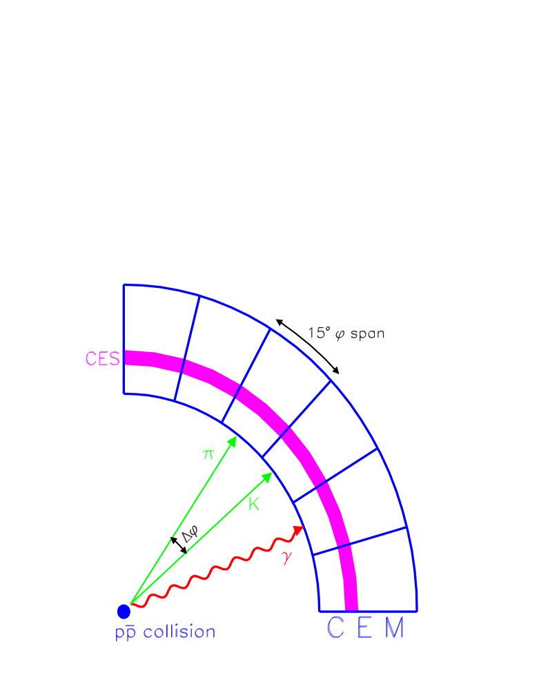
The CFT track processor was then used to select topologies suggestive of a penguin decay, with its photon and two charged hadrons. No track found by the CFT was allowed to point at the the same $\phi$ as the photon calorimeter tower (spanning $15^{\circ}$ in $\phi$). Two oppositely charged tracks with $p_{T}>2\;{\rm GeV}/c$ were sought close to the photon (within two calorimeter towers) and they were required to lie within $18^{\circ}$ of one another in $\phi$. Figure 2 illustrates the trigger topology. These track-related requirements were $\sim 35\%$ efficient for selecting penguin events while reducing the trigger cross section to $\sim 80\;{\rm nb}$.

When the trigger rate exceeded the limit of the data taking rate we further reduced the trigger rate by rejecting some fraction of the events which satisfied the trigger requirement (“prescale”). The second-level trigger was prescaled by a factor of two whenever the instantaneous luminosity was above $\sim 21\times 10^{30}\;{\rm cm^{-2}s^{-1}}$. The data loss due to the prescale, however, was minimal: this trigger considered $(22.3\pm 0.9)\;{\rm pb}^{-1}$ out of the $\sim 23\;{\rm pb}^{-1}$ of data available to it.

Events satisfying the second-level trigger were then passed to the third-level trigger for further consideration. The photon candidate’s electromagnetic $E_{T}$, reevaluated with clustering software, was required to be at least $7\;{\rm GeV}$, with an associated hadronic energy deposition of no more than 15% of that in the CEM. The profiles of energy deposition in the CEM and CES were also required to be consistent with expectations based on test beam results for electrons. The track cuts applied by the second-level trigger were confirmed at this trigger level using offline beam-constrained tracking in the CTC.

The open points of Figure 3 show the penguin trigger rates as a function of instantaneous luminosity during Run IB. These rates can be compared with the total trigger rates at each trigger level, shown by the closed points. From this figure we see that one out of 200 events accepted by the generic level-one calorimeter trigger also satisfied the second-level penguin trigger. The third-level trigger requirements provided an additional rate reduction by a factor of 6.5. Approximately 300000 events were collected during Run IB by the penguin trigger. The overall trigger efficiency for penguin decays resulting from B mesons with $p_{T}>12$ GeV/c and $|y|<1.25$ was $(1.7\pm 0.2)\%$ for $B_{d}\to K^{*0}\gamma$ and $(2.6\pm 0.3)\%$ for $B_{s}\to\phi\gamma$ decays. In the data sample collected by the penguin trigger in RunIB we expect around 7 $B_{d}\to K^{*0}\gamma$ and 2.6 $B_{s}\to\phi\gamma$ events. This sample was further refined in the offline analysis by selecting photon candidates in the good fiducial areas of the calorimeter, and by requiring that full CTC track reconstruction revealed no three-dimensional track pointing to the cluster. The $E_{T}(\gamma)$ threshold was raised to $10\;{\rm GeV}$. The hadronic/electromagnetic energy ratio selection was tightened to 10%, and requirements on shower profile consistency were also tightened.

The trigger thresholds for the penguin trigger were lowered for the 1995-96 data-taking period (“Run IC”). At the first trigger level, the $E_{T}$ threshold was lowered to $5\;{\rm GeV}$, raising the cross section to $\sim 30\;\mu{\rm b}$. The second-level energy requirements were lowered to $6\;{\rm GeV}$ in the CEM and $3\;{\rm GeV}$ in the CES while the relative hadronic energy and track topology requirements were kept the same. The trigger cross section at this level was thus raised to $\sim 500\;{\rm nb}$. The photon $E_{T}$ threshold was lowered to 5 GeV in the third-level trigger, while the other requirements were kept the same as in RunIB. Due to the lower photon energy requirements, the Run IC trigger acceptance rate was six times higher than the RunIB trigger, and the signal yield increased by a factor of five. As a result of these adjustments, approximately 500000 events were collected from the only $(6.6\pm 0.3)\;{\rm pb}^{-1}$ of Run IC integrated luminosity. The offline $E_{T}$ cut was accordingly lowered for this data to $8\;{\rm GeV}$.

A sample of electron candidates was also accumulated through Runs IB and IC. The trigger for this sample used the same first-level requirements as described above, but required $E_{T}>8\;{\rm GeV}$ at the second level, along with a CFT track with $p_{T}>7.5\;{\rm GeV}/c$ pointing to the EM cluster’s $\phi$ bin. At the third trigger level, the reevaluated thresholds were $E_{T}>7.5\;{\rm GeV}$ and $p_{T}>6\;{\rm GeV}/c$. Moreover, the track’s trajectory was extrapolated to the CES and compared with the shower positions; agreements within $\pm 3\;{\rm cm}$ in the azimuthal direction and $\pm 10\;{\rm cm}$ in $z$ were required. These trigger requirements were applied throughout Runs IB and IC.

The electron candidate sample serves two purposes in this analysis. In Method I we search for radiative decays among events selected by the penguin trigger. The electron sample provides a reference signal, $\overline{B}\rightarrow e^{-}D^{0}(\rightarrow K^{-}\pi^{+})X$, which we compare to the yield of radiative decay candidates. To facilitate this comparison, the same fiducial, $E_{T}$, and calorimeter requirements were applied offline to the subsample of the electron data which was collected concurrently with the penguin trigger; the uncertainties in the integrated luminosities of these two data sets are thus completely correlated. Because this reference sample was obtained by triggering on electrons, a single track was required to point to the electron cluster. Nevertheless, in order to simulate the penguin trigger requirements, no other track was allowed to point to that $\phi$ bin.

In Method II, where the photons are identified through their conversion to $e^{+}e^{-}$ pairs, the search for radiative decays is performed in the electron candidate sample itself. In this case, the offline selection applies fiducial, shower profile, and track-shower match requirements in a manner similar to Method I, but the $E_{T}$ threshold is lower at $8\;{\rm GeV}$. The minimum track $p_{T}$ is $6\;{\rm GeV}/c$. The hadronic/electromagnetic energy ratio requirement is tightened to 4% when only one track pointed to the cluster, but is left at 10% in cases with more than one track associated with the cluster. This sample also provided the reference signal, $B^{+}\rightarrow J/\psi(\rightarrow e^{+}e^{-})K^{+}$, and thus the entire Run IB data set is used for this method. The electron trigger accumulated $74\;{\rm pb}^{-1}$ during this period, amounting to approximately 3 million events satisfying the offline criteria.

IV Method I: Photon Trigger

In this section, we describe the search for $\overline{B}_{d}^{0}\rightarrow\overline{K}^{*0}(\rightarrow K^{-}\pi^{+})\gamma$ and $\overline{B}_{s}^{0}\rightarrow\phi(\rightarrow K^{+}K^{-})\gamma$ decays using the penguin trigger described in the previous section. The sensitivity of this method to $\Lambda_{b}^{0}\rightarrow\Lambda(\rightarrow p\pi^{-})\gamma$ is strongly reduced by the trigger requirement of $p_{T}>2$ GeV/$c$ for the pion track, because in the $\Lambda\to p\pi$ decays the proton carries most of the momentum of its parent and the pion is very slow. Thus, we do not attempt to reconstruct such decays. We derive the branching fraction limits for the radiative $B$ decays from the ratios between the numbers of candidate events and events of the reference signal, $\overline{B}\rightarrow e^{-}D^{0}(\rightarrow K^{-}\pi^{+})X$, found in the single electron data set.

A Radiative Decay Reconstruction

We selected candidate daughters of the $\overline{K}^{*0}$ and $\phi$ mesons from the radiative $B$ decays by asking for two oppositely charged tracks reconstructed with the inclusion of at least three hits in the SVX. Each track was required to have been found by the trigger system and have $p_{T}>2\;{\rm GeV}/c$. The penguin trigger topology requirements on the tracks and the photon candidate were reinforced offline. We then constrained each pair of candidate tracks to intersect at a common vertex and required the confidence level (CL) of the constrained fit to exceed 1%.

We retained two-track combinations consistent with $\overline{K}^{*0}\rightarrow K^{-}\pi^{+}$ by requiring $|M(K^{-}\pi^{+})-M_{\overline{K}^{*0}}|<80\;{\rm MeV}/c^{2}$, where $M_{\overline{K}^{*0}}$ is the world average $\overline{K}^{*0}$ mass ($896.1\;{\rm MeV}/c^{2}$) [4]. This window, corresponding to three times the natural $\overline{K}^{*0}$ width, contained more than $85\%$ of the $\overline{K}^{*0}$ signal. If the track pair also fell within the mass window when the $K$ and $\pi$ mass assignments were switched, we chose the assignment which yielded the two-track mass closer to the world average. This approach yielded the correct assignment 88% of the time. For $\phi\rightarrow K^{+}K^{-}$ decays, we required $|M(K^{+}K^{-})-M_{\phi}|<10\;{\rm MeV}/c^{2}$, where $M_{\phi}$ is the world average $\phi$ mass ($1019.4\;{\rm MeV}/c^{2}$) [4]. This window, corresponding to four times the natural $\phi$ width, contained $86.5\%$ of the $\phi\to K^{+}K^{-}$ signal.

In order to reject $K^{0}\rightarrow\pi^{+}\pi^{-}$ decays, we assigned pion masses to the two tracks and required that $|M(\pi^{+}\pi^{-})-M_{K^{0}}|>15\;{\rm MeV}/c^{2}$. We thus rejected combinations with masses within $2\sigma$ of the world average $K^{0}$ mass and retained 95.4% of the $\overline{K}^{*0}\rightarrow K^{-}\pi^{+}$ decays and all of the $\phi\rightarrow K^{+}K^{-}$ decays.

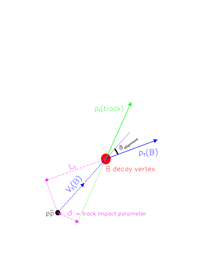
The track pair was combined with the photon candidate by adding their four-momenta. The trajectory of the photon candidate was determined by assuming that it originated from the $p\overline{p}$ vertex closest in $z$ to the track pair vertex; we call this $p\overline{p}$ vertex “primary.” Because the lifetimes of the $\phi$ and $\overline{K}^{*0}$ mesons are almost ten orders of magnitude smaller than that of the $B$ meson [4], the common fitted vertex of the two charged tracks indicated the point where the parent $B$ meson decayed. We computed the $B$ meson’s signed decay length $L_{T}=\vec{V}_{T}\cdot\vec{p}_{T}/p_{T}$, where $\vec{V}_{T}$ is the displacement in the transverse plane of the $B$ decay vertex with respect to the primary vertex (see Figure 4), and $\vec{p}_{T}$ is the $B$ meson momentum projected on the same plane. The proper decay length $ct$ could then be calculated with $ct=L_{T}\cdot(M/p_{T})$, where $M$ is the reconstructed mass of the $B$ meson candidate. The typical $ct$ resolution was $100\;\mu{\rm m}$. We required $0<ct<3\;{\rm mm}$, which retained 90% of the signal while rejecting half of the fake $B$ meson candidates formed by tracks coming directly from the primary vertex.

We further required that the $B$ meson carry most of the momentum in its vicinity. We defined the isolation variable

$$I_{B}\equiv\frac{p_{T}(B)}{p_{T}(B)+\sum_{\Delta R\leq 1}p_{T}}\,,$$ (1)

where the sum is over tracks consistent with originating from the primary vertex and within $\Delta R\equiv\sqrt{(\Delta\eta)^{2}+(\Delta\phi)^{2}}<1$ of the $B$ candidate trajectory. The $B$ candidate daughters were excluded from the sum. We required $I_{B}>0.7$. Studies with reconstructed $B$ decays in data indicate that this requirement is $\sim 95\%$ efficient in selecting real $B$ mesons of $p_{T}>15\;{\rm GeV}/c$ while rejecting half of the combinatorial background.

The mass resolution of $B$ mesons reconstructed in the above manner is given by simulation to be $110\;{\rm MeV}/c^{2}$, dominated by the energy resolution of the photon. We have used $D^{0}\rightarrow K^{-}\pi^{+}$ and electrons from the reference signal $\overline{B}\rightarrow e^{-}D^{0}X$ to verify that the simulation closely reproduces the momentum resolution and impact parameter resolutions of tracks, as well as the energy resolution and shower characteristics of electromagnetic objects. After the above selection criteria, there are $\sim 400$ $\overline{K}^{*0}\gamma$ and $\sim 40$ $\phi\gamma$ events within $220\;{\rm MeV}/c^{2}$ of the world average $\overline{B}_{d}^{0}$ and $\overline{B}_{s}^{0}$ masses of $5279\;{\rm MeV}/c^{2}$ and $5369\;{\rm MeV}/c^{2}$ respectively [4].

To further improve our sensitivity to the radiative decays, we exploited the long $B$ meson lifetime and the fact that we reconstructed all its daughters. The long lifetime resulted in large impact parameters for the $\overline{K}^{*0}$ and $\phi$ daughters with respect to the primary vertex; we cut on the significance of the impact parameters in the transverse plane, $|d/\sigma_{d}|$. The impact parameter resolution was typically $\sigma_{d}\sim 30\;\mu{\rm m}$. We also formed an “alignment angle” between the transverse momentum $\vec{p}_{T}$ and the displacement $\vec{V}_{T}$ of the $B$ meson candidate (see Figure 4):

$$\vartheta_{{\rm align}}\equiv\cos^{-1}\left(\frac{\vec{p}_{T}\cdot\vec{V}_{T}}{|\vec{p}_{T}|\cdot|\vec{V}_{T}|}\right).$$ (2)

Since we fully reconstructed the $B$ meson, real mesons yielded small values of $\vartheta_{{\rm align}}$, whereas the combinatorial background peaked away from zero. As a pure background sample we used events in the high mass region $6<M(\overline{K}^{*0}\gamma,\phi\gamma)<10\;{\rm GeV}/c^{2}$, where no real $B$ mesons should be found. Comparing the $\theta_{align}$ distributions of the simulated signal events with the distribution obtained from the background sample, we selected signal-like events by demanding $\theta_{align}<0.15$ rad, for both the $\overline{B_{d}}$ and $\overline{B_{s}}$ decays. We subsequently found the impact parameter significance cut which gave the highest signal-to-background efficiency ratio. It turned out that the best value was the one which rejected all events in the background (high mass) region.

The optimized selection cuts for $\overline{B}_{d}^{0}$ radiative decays were $\vartheta_{{\rm align}}<0.15\;{\rm rad}$ and $|d/\sigma_{d}|~{}>~{}5$. These requirements were 66% efficient in retaining $\overline{B}_{d}^{0}\rightarrow\overline{K}^{*0}\gamma$ decays. For the $\overline{B}_{s}^{0}$ decays, the narrower $\phi$ resonance, compared to the $\overline{K}^{*0}$, resulted in a smaller number of combinatorial background events falling within the, consequently narrower, mass window used to select the relevant two-track pairs. Thus, the optimized $|d/\sigma_{d}|$ cut for the $\overline{B}_{s}^{0}$ was less strict at $|d/\sigma_{d}|>2.5$. These optimized requirements are 69% efficient in retaining $\overline{B}_{s}^{0}\rightarrow\phi\gamma$ decays.

All together, the offline analysis requirements were $14.7\%$ ($8.3\%$) efficient in selecting $\overline{B}_{d}^{0}\rightarrow\overline{K}^{*0}\gamma$ decays which already satisfied the trigger requirements in Run IB (Run IC). The respective efficiencies for $\overline{B}_{s}^{0}\rightarrow\phi\gamma$ decays were $12.9\%$ in Run IB and $7.2\%$ in Run IC. The Run IC efficiencies were lower than Run IB because the offline cut for the photon energy was placed at $E_{T}>8\;{\rm GeV}$, instead of the $6\;{\rm GeV}$ trigger threshold, in order to match the energy threshold of the electrons used to reconstruct the reference channel.

Figure 5 shows the invariant mass distributions of the three-body combinations surviving all the selection criteria. The $\pm 220\;{\rm MeV}/c^{2}$ signal region around the world average $B$ mass is double-hatched in the figure, and the sideband regions, $3.9<M(\overline{K}^{*0}\gamma)<4.9$ and $5.7<M(\overline{K}^{*0}\gamma)<6.7\;{\rm GeV}/c^{2}$, are single-hatched. One $\overline{B}_{d}^{0}\rightarrow\overline{K}^{*0}\gamma$ candidate, from the Run IC sample, remains in the signal region, while five populate the sidebands. The expected background in the signal region, assuming a uniform distribution interpolated between the sidebands, is $N_{{\rm bg}}=1.1\pm 0.5$ events. There are 2 events just outside the signal window. However, the probability of them being signal is small.

In the $\overline{B}_{s}^{0}\rightarrow\phi\gamma$ case, no candidates survive the selection cuts. Since there are also no events in the $\overline{B}_{s}^{0}$ sidebands, in the signal region we expect $N_{{\rm bg}}<0.54$ events with $90\%$ confidence [4], assuming a uniform distribution interpolated between the sidebands.

B Reference Signal Reconstruction

We reconstructed our reference sample of $\overline{B}\rightarrow e^{-}D^{0}(\rightarrow K^{-}\pi^{+})X$ decays, by adding the four-momenta of the two tracks and the electron candidate. For $e+D^{0}$ combinations from $B$ decays, we expected the kaon from the $D^{0}$ to have the same charge as the electron. The mass assignment of the pion and kaon masses to the two tracks was thus uniquely determined.

We retained $\overline{B}\rightarrow e^{-}D^{0}(\rightarrow K^{-}\pi^{+})X$ candidates with a $p_{T}(B)$ distribution similar to that of the radiative decay candidates by requiring $p_{T}(eK\pi)>15\;{\rm GeV}/c$ in Run IB. For Run IC, this threshold was lowered to $13.5\;{\rm GeV}/c$ to accommodate the lower photon threshold. We also required that the mass of the three-body combination $M(eK\pi)$ be less than $5\;{\rm GeV}/c^{2}$. Finally, we applied the same $0<ct<3\;{\rm mm}$ and $I_{B}>0.7$ requirements as on the radiative decay candidates. These semileptonic decays, however, were not fully reconstructed, and we used the combined momentum of the $e+D^{0}$ system for the (pseudo-proper) lifetime calculation. In addition, rather than extrapolating the $D^{0}$ decay vertex to the trigger electron track in order to locate the $B$ decay vertex, we simply used the $D^{0}$ decay vertex for the calculation of $ct$ to avoid additional systematic uncertainties due to the further vertex reconstruction.

We then required $|d/\sigma_{d}|>3$ for the kaon and pion tracks from the $D^{0}\rightarrow K^{-}\pi^{+}$ decay. Since $\overline{B}\rightarrow e^{-}D^{0}X$ decays are not fully reconstructed, we do not make a $\vartheta_{{\rm align}}$ cut. The invariant masses of the selected $K^{-}\pi^{+}$ combinations from $\overline{B}\rightarrow e^{-}D^{0}X$ candidates are shown in Figure 6. The $K^{-}\pi^{+}$ combinations with the wrong charge correlation with the electron are also shown. We estimated the number of $\overline{B}\rightarrow e^{-}D^{0}X$ candidates by fitting the data with a Gaussian signal and a linear background and we found $40.7\pm 7.3$ events in Run IB and $27.4\pm 6.2$ events in Run IC.

C Efficiencies

In method I we infer the radiative decay branching fraction from a measurement of its ratio with the known $\mbox{${\cal B}$}(\mbox{$\overline{B}\to e^{-}D^{0}X$})$. The $b$-quark production cross section cancels in the ratio, while the effect of systematic uncertainties is reduced. We write for $\overline{B}_{d}^{0}\to\overline{K}^{*0}\gamma$ ,

$$\mbox{${\cal B}$}(\mbox{$\overline{B}_{d}^{0}\to\overline{K}^{*0}\gamma$})=\mbox{${\cal B}$}(\mbox{$\overline{B}\to e^{-}D^{0}X$})\times\frac{N_{K^{*0}\gamma}}{N_{eD^{0}}}$$ (3)

$$\times\left[\frac{f_{d}}{f_{u}+f_{d}}\frac{\mbox{${\cal B}$}(\mbox{$\overline{K}^{*0}\to K^{-}\pi^{+}$})}{\mbox{${\cal B}$}(\mbox{$D^{0}\to K^{-}\pi^{+}$})}\frac{\epsilon_{K^{*0}\gamma}}{\epsilon_{eD^{0}}}\frac{L_{\rm peng}}{L_{eX}}\right]^{-1},$$ (4)

and for $\overline{B}_{s}^{0}\to\phi\gamma$ ,

$$\mbox{${\cal B}$}(\mbox{$\overline{B}_{s}^{0}\to\phi\gamma$})=\mbox{${\cal B}$}(\mbox{$\overline{B}\to e^{-}D^{0}X$})\times\frac{N_{\phi\gamma}}{N_{eD^{0}}}$$ (6)

$$\times\left[\frac{f_{s}}{f_{u}+f_{d}}\frac{\mbox{${\cal B}$}(\mbox{$\phi\to K^{+}K^{-}$})}{\mbox{${\cal B}$}(\mbox{$D^{0}\to K^{-}\pi^{+}$})}\frac{\epsilon_{\phi\gamma}}{\epsilon_{eD^{0}}}\frac{L_{\rm peng}}{L_{eX}}\right]^{-1},$$ (7)

where $\left.N_{K^{*0}\gamma,\phi\gamma}\right/N_{eD^{0}}$ is the ratio of the observed number of events of the radiative decays and $\overline{B}\to e^{-}D^{0}X$, $\left.\epsilon_{K^{*0}\gamma,\phi\gamma}\right/\epsilon_{eD^{0}}$ is the ratio of the efficiencies, and $\left.L_{\rm peng}\right/L_{eX}$ is the ratio of the integrated luminosities of the penguin and the inclusive electron data samples. We assume that the composition of $\overline{B}\to e^{-}D^{0}X$ candidates is only $B_{u}^{-}$ and $\overline{B}_{d}^{0}$, and thus the ratios of the fragmentation fractions are $f_{d,s}/(f_{u}+f_{d})$, neglecting the small contributions from other $b$ hadrons such as $\overline{B}_{s}^{0}$ and $\Lambda_{b}^{0}$ to the denominator. We note that the contribution of the $\overline{B}_{s}^{0}$ through the $\overline{B}_{s}^{0}\rightarrow e^{-}\overline{\nu}_{e}D_{s}^{**}\rightarrow e^{-}D^{0}X$ decay is estimated to be less than 3% in the $e+D^{0}$ sample. The branching fractions [4] and fragmentation fractions [20] used in this analysis are listed in Table I.

Since we use electron trigger data collected concurrently with the penguin trigger data, the integrated luminosities of $p\bar{p}$ collisions are the same for the two data sets. The effective integrated luminosities of each data set, however, are different for the two due to the different prescale factors. The true integrated luminosities for the penguin and electron data set are 22.3 pb^-1 and 16.2 pb^-1, respectively, in Run IB, and 6.6 pb^-1 and 4.2 pb^-1 in IC. We assume that all the uncertainties cancel in the ratio.

The efficiency ratios were evaluated using a combination of simulation and data. We employed a Monte Carlo simulation of events with a single $b$ quark to calculate the efficiencies of the kinematic and topological requirements imposed on the data. In this simulation, the $b$ quarks were generated with a rapidity and momentum distribution based on a next-to-leading order QCD calculation [21] that used the MRSD0 parton distribution functions [22] and a renormalization scale of $\mu=\mu_{0}\equiv\sqrt{m_{b}^{2}+p_{T}^{2}}$, where $m_{b}=4.75\;{\rm GeV}/c^{2}$ is the mass of the $b$ quark and $p_{T}$ is its transverse momentum. These $b$ quarks were subsequently hadronized into $B$ mesons using the Peterson fragmentation function [23] with a fragmentation parameter $\epsilon_{b}=0.006$. The resulting $B$ mesons were then decayed through the channel of interest using the QQ Monte Carlo program [24] to model the phase space, helicity, and angular distributions of the decay products.

For the reference channel, we generated different samples for each of the contributing decay chains: $\overline{B}\rightarrow e^{-}\overline{\nu}_{e}D^{0}$; $\overline{B}\rightarrow e^{-}\overline{\nu}_{e}D^{*}(\rightarrow D^{0}X)$; $\overline{B}\rightarrow e^{-}\overline{\nu}_{e}D^{**}(\rightarrow D^{0}X)$; and $\overline{B}\rightarrow e^{-}\overline{\nu}_{e}(Dn\pi)_{{\rm nr}}$ followed by $(Dn\pi)_{{\rm nr}}\rightarrow D^{0}X$, where $(Dn\pi)_{{\rm nr}}$ indicates a $D$ meson produced in non-resonant association with extra pions. We then mixed these semileptonic samples according to their relative abundances and selection efficiencies to create a representative $\overline{B}\rightarrow e^{-}D^{0}X$ sample. We fed these events through the detector and trigger simulations to obtain the efficiencies. We also used this simulation to calculate the relative effects of the photon/electron trigger cuts, the offline quality cuts, and the track reconstruction in the SVX. We considered simulated SVX track reconstruction since the SVX simulation incorporated the same hit efficiencies and pattern recognition as the data.

Second-level trigger efficiencies were studied using data. The efficiency of the CES energy requirement was parameterized as a function of electron or photon $E_{T}$ by analyzing electrons in a very pure sample derived from photon conversions. Applying this parameterization to the Monte Carlo samples, we find all the efficiencies to be around 95%. The efficiency ratios are therefore near unity, and the 2% uncertainty in the ratio is included in the systematic uncertainty.

The efficiency of the CFT trigger requirements for kaons and pions was determined as a function of track $p_{T}$. We found the CFT is 50% efficient at $1.9\;{\rm GeV}/c$ and 90% efficient at $2.4\;{\rm GeV}/c$. The efficiency function of the CFT trigger requirements for the electron in the reference signal was determined using a heavily prescaled electron data set with a lower energy threshold and no CFT requirement; 50% efficiency is reached at $6.0\;{\rm GeV}/c$ and 90% at $10.0\;{\rm GeV}/c$. The plateau efficiency is $0.915\pm 0.010$. These efficiency parameterizations were applied to the Monte Carlo samples to study the effect on the ratios of efficiencies.

The offline CTC tracking efficiencies for kaons and pions were estimated by embedding Monte Carlo-generated tracks into real $J/\psi\rightarrow\mu^{+}\mu^{-}$ events [25]. The efficiency rises with $p_{T}$ in the range $200<p_{T}<400\;{\rm MeV}/c$, and plateaus at a value which depends on the instantaneous luminosity and the charge of the track. The integrated efficiency for tracks with $p_{T}>400\;{\rm MeV}/c$ is $0.96\pm 0.02$. Again, we applied the efficiency parameterization to Monte Carlo samples of the decays of interest. For $\overline{K}^{*0}\rightarrow K^{-}\pi^{+}$ and $\phi\rightarrow K^{+}K^{-}$ decays with the requirement $p_{T}>2\;{\rm GeV}/c$ for the kaons and pions, the efficiency of offline CTC tracking was found to be $0.94\pm 0.04$. The corresponding efficiency for the $K^{-}\pi^{+}$ combinations from the $D^{0}$ decays is $\sim 1\%$ lower due to the lower $p_{T}$ of the tracks. The uncertainties in these efficiencies are dominated by the instantaneous luminosity dependence of the tracking efficiency and thus cancel in the efficiency ratio. The offline tracking efficiency for the trigger electron in the reference signal was estimated using an independent electron data sample to be $0.99\pm 0.01$. We therefore estimate the ratio of tracking efficiencies for both $K^{*0}\gamma$ and $\phi\gamma$, relative to the reference signal, to be $1.02\pm 0.02$.

The effect of the isolation requirements for the trigger photon or electron, as well as the $I_{B}>0.7$ cut for the $B$ meson, depends strongly on the environment of the $B$ decay (e.g., $b$ fragmentation, or multiple $p\overline{p}$ interactions). We expect similar environments around the $B$ mesons in the reference and radiative decay processes and consequently the efficiencies are nearly equal. Small differences can be expected due to the extra particles produced in $\overline{B}\rightarrow e^{-}D^{0}X$ decays and because the reference signal contains $B^{-}$ mesons along with $\overline{B}^{0}$. We simulated the full $p\overline{p}\rightarrow b\overline{b}$ environment using the PYTHIA Monte Carlo generator, tuned to match the underlying charged particle distributions in $\overline{B}\rightarrow\ell^{-}D^{0}X$ data [26]. We fed these events through the detector and trigger simulations and found that the isolation efficiencies are somewhat higher for the radiative decay channels than for the reference signal; the ratio is $1.04\pm 0.02$ for $\overline{B}_{d}^{0}\rightarrow\overline{K}^{*0}\gamma$ and $1.06\pm 0.02$ for $\overline{B}_{s}^{0}\rightarrow\phi\gamma$.

Taking all the efficiencies into account, we find that the efficiency ratios between the radiative decays and the reference channel are $\epsilon_{K^{*0}\gamma}/\epsilon_{eD^{0}}=2.7$ in Run IB and 2.0 in Run IC. In the $\overline{B}_{s}^{0}\rightarrow\phi\gamma$ case, we find these ratios to be 3.5 in Run IB and 2.5 in Run IC.

Table I summarizes the elements of the branching fraction calculation for each of the decay modes investigated here. The table also shows the “single event sensitivity” $S$ for the two penguin decay modes. $S$ is defined here as

$$S=\frac{{\rm branching\;fraction}}{{\rm observed\;number\;of\;events}}$$ (8)

and can be rewritten with the known quantities by using Eqs. 3 and 6. This quantity represents the branching fraction which would result in an average of one event being observed in this analysis. The difference in the sensitivities between the $\overline{B}_{d}^{0}\rightarrow\overline{K}^{*0}\gamma$ and $\overline{B}_{s}^{0}\rightarrow\phi\gamma$ decay modes is dominated by the difference of the $b$ quark hadronization fractions.

D Systematic Uncertainties

Table II lists the sources of systematic uncertainty considered in this analysis. The largest contribution to the total is the uncertainty on the yield of $\overline{B}\rightarrow e^{-}D^{0}(\rightarrow K^{-}\pi^{+})X$ decays, which is 18% in Run IB and 23% in Run IC. The second largest contribution arises from the uncertainty in the measurement of $f_{s}/(f_{u}+f_{d})$ [20], followed by the uncertainty in the product of branching fractions ${\cal B}(\overline{B}\rightarrow e^{-}D^{0}X)\cdot{\cal B}(D^{0}\rightarrow K^{-}\pi^{+})$.

The last significant contribution to the systematic uncertainty comes from the fraction of the time when the $D^{0}$ meson from a $\overline{B}$ decay is not an immediate daughter of the $\overline{B}$ meson but is instead a decay product of an intermediate excited $D$ state. Depending on how far down the decay chain of the $\overline{B}$ meson the $D^{0}$ appears, the kinematics of the resulting kaon and pion, and hence the reconstruction efficiencies, are different. In the Monte Carlo simulation used to determine the efficiency ratios, the nominal fractions of $D^{0}$ mesons coming from $D^{**}$ mesons and $(Dn\pi)_{{\rm nr}}$ states ($f^{**}$), from $D^{*}$ mesons ($f^{*}$), and directly from the $\overline{B}$ meson ($f$) were $f^{**}:f^{*}:f=0.35:0.53:0.12$ [4]. These fractions were varied to $0.24:0.62:0.14$ and $0.47:0.43:0.10$. We observed a 12% variation in the efficiency in Run IB and 11% in Run IC. We take these variations as the systematic uncertainties in the efficiency ratios.

The rest of the systematic uncertainty contributions have little effect on the total, which is about 30%. For instance, the Monte Carlo efficiency estimates depend on their input distributions, such as the $p_{T}$ distribution of the incident particles. We re-weight the Monte Carlo $p_{T}(B)$ distribution which is used as the simulation input by the ratio of the measured $B$ production cross section [27] to the theoretical prediction. Even though the efficiencies for individual channels vary by as much as $\sim 20\%$, the ratios of efficiencies do not change by more than 5%.

Another relatively small effect is the uncertainty in the difference in trigger efficiencies for photons and electrons. The difference resulting from the different $E_{T}$ spectra of the photons and electrons is accounted for in the Monte Carlo calculation; moreover, we confirm that the detector simulation indeed reproduces the characteristics of the electromagnetic shower profile using $\overline{B}\rightarrow e^{-}D^{0}X$ decays in data. We nevertheless assign an uncertainty due to the $E_{T}$ differences between the reference channel electron and the radiative decay photon to allow for uncertainties in the simulation of the electromagnetic energy clustering at the trigger level. We study the effect of varying the relative efficiency by re-weighting the photon and electron $E_{T}$ distribution in the lowest 10 GeV, away from the efficiency plateau, by as much as a factor of two (e.g., the weight is applied for $10<E_{T}<20$ GeV in Run IB). No weighting is applied for energies in the plateau region. Such a modification of the threshold induces a change in the individual event rates by as much as 50%, but the ratio varies by only $\sim 8\%$, which we take as the systematic uncertainty.

The efficiency of the CES trigger requirement itself is measured with an uncertainty of $\sim 1.5\%$. Assuming that the efficiency for electrons is uncorrelated with that of the radiative decay photons, we obtain a conservative 2% systematic uncertainty from this source.

The CFT efficiency was measured with an uncertainty of $\sim 1.5\%$ for kaons and pions, and 1% for electrons. Due to the spatial proximity of the two tracks in the radiative decays, we consider their efficiencies to be 100% correlated and thus assign a 3% uncertainty for the efficiency ratio. Another 2% uncertainty comes from the CTC tracking efficiency, 2% from the differences in the isolation efficiencies, and 2% from the finite size of the Monte Carlo samples used to calculate the efficiency ratios.

The uncertainties listed above were combined in quadrature to obtain the total systematic uncertainties on the branching fractions of the radiative decays. As shown in Table II, the total is $\sim 30\%$ for $\overline{B}_{d}^{0}$ and slightly higher for $\overline{B}_{s}^{0}$.

We combine the Run IB and IC systematic uncertainties by assuming that the uncertainties due to the statistics of the $e+D^{0}$ candidates and Monte Carlo samples are uncorrelated, and any other sources are fully correlated. The uncorrelated systematic uncertainties are added in quadrature, while the fully correlated ones are simply added. The total systematic uncertainties are 25% for $\overline{B}_{d}^{0}$ and 31% for $\overline{B}_{s}^{0}$ radiative decays.

E Results

Since we observe no significant signal for either $\overline{B}_{d}^{0}$ or $\overline{B}_{s}^{0}$ radiative decays, we set upper limits for their branching fractions. We use a conservative procedure which ignores possible background contributions to the observed event yields.

First, we calculate an upper limit on the mean number of radiative decays $N_{{\rm CL}}$ at a given CL, including the total systematic uncertainty $\sigma_{{\rm syst}}$, by numerically solving the following equation:

$$1-{\rm CL}=\sum_{n=0}^{N_{{\rm obs}}}{\cal P}_{N_{{\rm CL}},\sigma_{{\rm syst}}}(n),$$ (9)

where $N_{{\rm obs}}$ is the number of candidates observed, and ${\cal P}_{\mu,\sigma}(n)$ is defined with the Poisson distribution $P_{\mu}(n)$ and the Gaussian distribution $G_{\mu,\sigma}(x)$ as follows:

$${\cal P}_{\mu,\sigma}(n)=\int_{0}^{\infty}P_{x}(n)G_{\mu,\sigma}(x)dx.$$ (10)

With one $\overline{B}_{d}^{0}\to\overline{K}^{*0}\gamma$ candidate observed in the entire data sample and a 25% uncertainty, the upper limit on the mean number of radiative decays is 4.3 (5.5) at 90% (95%) CL. This result, with a single event sensitivity (Equation 8) of $3.8\times 10^{-5}$, yields upper limits on the branching fraction $\mbox{${\cal B}$}(\mbox{$\overline{B}_{d}^{0}\to\overline{K}^{*0}\gamma$})$ of $1.6\times 10^{-4}$ at 90% CL and $2.1\times 10^{-4}$ at 95% CL. With no $\overline{B}_{s}^{0}\to\phi\gamma$ candidates and a total uncertainty of 31%, we expect less than 2.6 (3.6) events on average at 90% (95%) CL. With a single event sensitivity of $9.3\times 10^{-5}$, we thus obtain $\mbox{${\cal B}$}(\mbox{$\overline{B}_{s}^{0}\to\phi\gamma$})<2.5\times 10^{-4}$ at 90% CL and $<3.3\times 10^{-4}$ at 95% CL.

V Method II: Photon Conversion

In this section, we describe the search for $\overline{B}_{d}^{0}\rightarrow\overline{K}^{*0}(\rightarrow K^{-}\pi^{+})\gamma$, $\overline{B}_{s}^{0}\rightarrow\phi(\rightarrow K^{+}K^{-})\gamma$, and $\Lambda_{b}^{0}\rightarrow\Lambda(\rightarrow p\pi^{-})\gamma$ decays in which the photon is identified by an electron-positron pair produced through photon conversion before reaching the CTC volume. A conversion daughter with $E_{T}>8\;{\rm GeV}$ served as the trigger; the same inclusive electron trigger was used for the $e+D^{0}$ sample in Method I.

Though the typical photon conversion probability was 6% for CDF in this data, this analysis benefits from the fact that we can utilize all of the Run IB data, which corresponds to an integrated luminosity of $74\;{\rm pb}^{-1}$, or three times more than that collected with the penguin trigger, and that there was no requirement of any additional tracks at the trigger level. This fact allowed us to apply, in the offline selection, a $p_{T}$ threshold as low as $0.5\;{\rm GeV}/c$ to the hadron tracks coming from the $b$ hadron decays instead of the $2\;{\rm GeV}/c$ cut used in Method I. This lower threshold essentially doubles the efficiency for the $B$ hadron decay products. Moreover, in the relatively low energy region of our interest where the tracking has better resolution than the calorimetry, reconstructing $b$ hadron masses from the momenta measured by the tracking detectors has the advantage of good mass resolution. This is typically $45\;{\rm MeV}/c^{2}$ for the reconstructed $B$ mesons and is dominated by the momentum resolution of the trigger electron.

We derive the branching fractions for the radiative $b$ hadron decays from the ratios between the numbers of such decays and $B_{u}^{-}\rightarrow J/\psi(\rightarrow e^{+}e^{-})K^{-}$ decays found in the same data set. The uncertainties in the $b$ quark production cross section and on the integrated luminosity thus cancel, as well as most of the uncertainties on the detection efficiency. It would have been preferable to use $\overline{B}_{d}^{0}\rightarrow J/\psi K^{*0}$, $\overline{B}_{s}^{0}\rightarrow J/\psi\phi$, and $\Lambda_{b}^{0}\rightarrow J/\psi\Lambda$ decays instead of $B_{u}^{-}\rightarrow J/\psi K^{-}$, since they arise from the same production mechanisms as the corresponding radiative decays and are topologically more similar. However our samples of those final states are too small to be useful as normalization.

A Radiative Decay Reconstruction

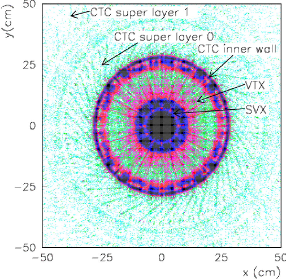
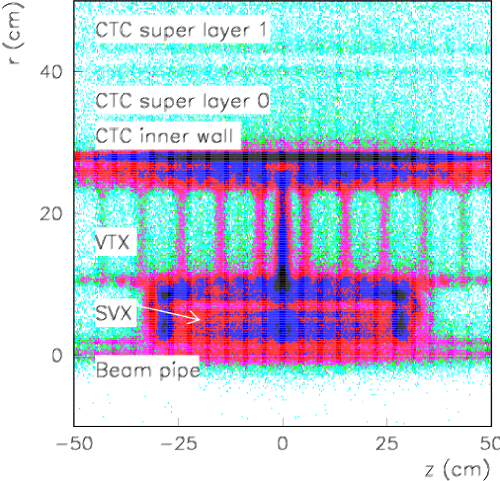
Reconstruction of the radiative decays began with identification of a photon conversion. A photon conversion candidate was formed by the electron candidate and an oppositely charged track with $p_{T}>0.5$ GeV/$c$. A fit was made which constrains the two tracks to originate from a common vertex and be parallel to each other at the vertex. The CL of the fit was required to be greater than 0.1%. The background due to misidentified electrons and combinatorial backgrounds is small ($<1\%$) among the photon conversion candidates with a vertex outside the beam pipe. The candidates that have their conversion points inside the beam pipe are dominated by real electron-positron pairs from Dalitz $\pi^{0}$ and $\eta$ decays. We required the transverse distance of the conversion point from the nominal beamline to be less than 30 cm in order to ensure that it is in the well known materials before the CTC, and to be greater than 3 cm in order to reject backgrounds from Dalitz decays. We obtained $\sim 850000$ photon conversion candidates in the Run IB data. Figures 7 and 8 show, for all transverse distances, the reconstructed conversion vertex density in the $x-y$ plane and $r-z$ plane. The fine structure of the CDF tracking detectors such as the SVX ($r\sim 5$ cm), the VTX ($r\sim 15$ cm), and the CTC ($r>30$ cm) can be clearly resolved. The detailed study of the CDF material distribution using $\sim 200000$ conversion candidates in 1992-1993 data is described in [28].

For each photon conversion candidate in an event, we searched for $\overline{B}_{d}^{0}\to\overline{K}^{*0}\gamma$ and $\overline{B}_{s}^{0}\to\phi\gamma$ decays. A $\overline{B}_{d}^{0}$ candidate was formed by the photon conversion candidate and a pair of oppositely charged tracks. The two “meson tracks” were required to be reconstructed in the SVX with hits in at least 3 layers. In addition, the transverse momenta had to exceed 0.5 GeV/$c$ for each track and 2 GeV/$c$ for the two-track system. A fit was performed with the following topological constraints: (1) the meson tracks originate from a common vertex; (2) the photon conversion candidate points back to the meson decay vertex; and (3) the four-track system points back to the primary vertex, which was defined to be the $p\bar{p}$ collision point nearest in $z$ to the trigger electron track’s closest approach to the beamline. We required the CL of the fit to be greater than 0.1%. The $\overline{B}_{d}^{0}$  candidate was then accepted if the reconstructed $\overline{K}^{*0}$  mass was within $\pm 80$ MeV/$c^{2}$ of the world average value. Both $K^{+}\pi^{-}$ and $\pi^{+}K^{-}$ mass assignments were considered for the $\overline{K}^{*0}$ candidate, and the assignment giving a value closer to the world average was chosen. We also required that the pseudorapidity of the $B$ candidate $|\eta_{B}|$ be less than 1. Finally, we selected candidates with lifetime $ct>100$ $\mu$m and $I_{B}>0.7$ (See Section IV A).

The selection of $\overline{B}_{s}^{0}$ candidate proceeded on similar lines, except both tracks were assigned kaon masses and the mass window was $\pm 10\;{\rm MeV}/c^{2}$ around the world average.

At this point, there were 15 $\overline{K}^{*0}\gamma$ and one $\phi\gamma$ events within $100\;{\rm MeV}/c^{2}$ of the corresponding world average $B$ masses. As previously noted, the mass resolution of the reconstructed $B$ mesons is about $45\;{\rm MeV}/c^{2}$. We refined this selection by tightening the $p_{T}$ cut on the two-track system and by applying impact parameter significance cuts to the individual meson tracks. The thresholds were optimized by maximizing $\epsilon_{{\rm sig}}/\sqrt{\epsilon_{{\rm bg}}}$, where $\epsilon_{{\rm sig}}$ and $\epsilon_{{\rm bg}}$ are the efficiencies for the signal and background events found in the $\pm 100\;{\rm MeV}/c^{2}$ window around the $B$ masses. The signal efficiency was obtained from Monte Carlo calculations similar to that of Method I (see Section IV C), while $\epsilon_{{\rm bg}}$ was estimated by interpolating the observed yields in the mass sidebands, defined to extend from 200 to $1200\;{\rm MeV}/c^{2}$ above and below the average mass, through the signal region. For the $\overline{B}_{d}^{0}$ channel, the optimized selection cuts were $p_{T}(K\pi)>2.75\;{\rm GeV}/c$ and $|d/\sigma_{d}|>4.5$ for both meson tracks. Figure 9(top) shows the $\overline{K}^{*0}\gamma$ mass distribution after these cuts. Any further cuts, for example on the proper decay length, did not improve $\epsilon_{{\rm sig}}/\sqrt{\epsilon_{{\rm bg}}}$. One candidate remained in the $\overline{B}_{d}^{0}$ signal region; the expected background is $0.6\pm 0.3$ events.

For the $\overline{B}_{s}^{0}$ channel, the optimized selection cuts were $p_{T}(KK)>2.25\;{\rm GeV}/c$ and $|d/\sigma_{d}|>3.0$. The resulting invariant mass distribution is shown in Figure 10(top). No candidates were found in the signal region, where we expected a background of $0.1\pm 0.1$ events.

The decay $\Lambda_{b}^{0}\rightarrow\Lambda(\rightarrow p\pi^{-})\gamma$ is topologically distinct from the meson decays. Since the $\Lambda$ has a long lifetime, with $ct\sim 8\;{\rm cm}$, it decays outside the SVX fiducial volume $\sim 85\%$ of the time, and thus only 15% of the $\Lambda$ decays are expected to have associated SVX tracks. We therefore first reconstructed $\Lambda$’s without using SVX information. The higher-$p_{T}$ track of the track pair was assumed to be the proton, and was required to have $p_{T}>1.5\;{\rm GeV}/c$ while the pion had to have $p_{T}>0.4\;{\rm GeV}/c$. The energy loss $dE/dx$ for both tracks had to be consistent with expectations. A vertex-constrained fit of the track pair was accepted if its CL exceeds 0.1%. Photon conversions, a major source of background for $\Lambda\rightarrow p\pi^{-}$ decays, were rejected here by eliminating those track pairs which could be fit with the conversion hypothesis. Finally, the track pair was accepted as a “CTC-$\Lambda$” candidate if the distance of the decay vertex from the nominal beamline exceeded $1\;{\rm cm}$.

If both the proton and pion tracks had at least two SVX hits, the vertex-constrained fit was redone using the SVX information. Again, the CL of the fit was required to be greater than 0.1%. We also required the SVX layer hit pattern to be consistent with the expectation from the reconstructed $\Lambda$ decay. For example, if the $\Lambda$ decay vertex was between the second and third of the four SVX layers, we required that the tracks have exactly two hits in the outermost layers. About 10% of the “CTC-$\Lambda$” candidates satisfied the above requirements and were thus reclassified as “SVX-$\Lambda$” candidates.

A $\Lambda_{b}^{0}$ candidate was formed by a photon conversion and a $\Lambda$ candidate. From the CTC-$\Lambda$ candidates, we reconstructed “CTC-$\Lambda_{b}^{0}$” candidates with a constraint that both the $\Lambda$ and the photon point back to the primary vertex. This constraint improved the $\Lambda_{b}^{0}$ mass resolution from $75\;{\rm MeV}/c^{2}$, without the constraint, to $50\;{\rm MeV}/c^{2}$. For the SVX-$\Lambda$ candidates, however, only the photon was constrained to point back to the primary vertex, while the $\Lambda$ trajectory was required only to point backwards to within $2\;{\rm cm}$ in $z$ of the primary vertex. The typical $\Lambda_{b}^{0}$ mass for these “SVX-$\Lambda_{b}^{0}$” candidates is also $50\;{\rm MeV}/c^{2}$. In both cases, we required the CL of the constrained fit to exceed 0.1%. We then recalculated the $\Lambda$ mass given the constraints and required that it fell within $\pm 3\;{\rm MeV}/c^{2}$ of the world average $\Lambda$ mass. The typical $\Lambda$ mass resolutions are $2.5\;{\rm MeV}/c^{2}$ for CTC-$\Lambda_{b}^{0}$ candidates, and $1.5\;{\rm MeV}/c^{2}$ for SVX-$\Lambda_{b}^{0}$.

We improved the sample purity by requiring large impact parameters, recalculated after the constrained fit, for the proton and pion tracks. In the SVX-$\Lambda_{b}^{0}$ case, the impact parameter resolution was good enough to require at least $3\sigma_{d}$ inconsistency with the primary vertex. In the CTC-$\Lambda_{b}^{0}$ case, however, we noted that the proton carries most of the momentum of its parent and required only $|d/\sigma_{d}|>0.5$ inconsistency. The pion from $\Lambda^{0}$ decay is more likely to have a large impact parameter, so we required $|d/\sigma_{d}|>2$. Finally, we selected $\Lambda_{b}^{0}$ pseudorapidity $|\eta_{\Lambda_{b}^{0}}|<1$ and isolation $I_{B}>0.7$, as before. After these selection cuts, we found 23 CTC-$\Lambda_{b}^{0}$ and 2 SVX-$\Lambda_{b}^{0}$ candidates in the $\pm 100\;{\rm MeV}/c^{2}$ window around the world average $\Lambda_{b}^{0}$ mass.

The SVX-$\Lambda_{b}^{0}$ candidates were further refined by considering the signed impact parameter of the $\Lambda$’s. The sign is defined as positive when the crossing point of the $\Lambda$ and the $\Lambda_{b}^{0}$ momenta lies in the hemisphere containing the $\Lambda_{b}^{0}$, as should be the case for real $\Lambda_{b}^{0}$ decays. The typical resolution of the signed impact parameter is $40\;\mu{\rm m}$. Following the same optimization procedure as before, we find that a cut value of $70\;\mu{\rm m}$ maximizes $\epsilon_{{\rm sig}}/\sqrt{\epsilon_{{\rm bg}}}$. No candidates survived this cut, while the expected background is $0.1\pm 0.1$ events.

Since the CTC-$\Lambda_{b}^{0}$’s lack the improved impact parameter resolutions of the SVX, we reinforced the kinematic requirements by requiring the $p_{T}$ of the $\Lambda$ to be greater than $4\;{\rm GeV}/c$. Two candidates remained in the signal region, and the expected background is $3.3\pm 0.6$ events. Combining the CTC and SVX samples, we found two candidates in the signal region with an expected background of $3.4\pm 0.6$ events. The invariant mass distribution is shown in Figure 11 (top).

B Reference Signal Reconstruction

The reference signal for this analysis method consists of $B_{u}^{-}\rightarrow J/\psi(\rightarrow e^{+}e^{-})K^{-}$ decays. A $J/\psi\rightarrow e^{+}e^{-}$ candidate was formed by the electron candidate and an oppositely charged track with $p_{T}>1\;{\rm GeV}/c$. We required the partner track to exhibit energy loss in the CTC and deposition in the CEM in a manner consistent with being an electron. The two tracks were then subject to a vertex-constrained fit, and its CL is required to be greater than 0.1%. The dielectron invariant mass distribution is shown in Figure 12. The ratio of signal to background $S/B$ is approximately 1/2 in the 2.8 to $3.2\;{\rm GeV}/c^{2}$ mass range. The backgrounds are mostly combinatorial, involving hadrons misidentified as the partner electron. The low-mass tail on the signal is due to photon bremsstrahlung on the electron tracks. A fit of the mass distribution with two Gaussians and a second-order polynomial yields $\sim 8000\;J/\psi\rightarrow e^{+}e^{-}$ events.

The $J/\psi$ candidates were then combined with a track with $p_{T}>2\;{\rm GeV}/c$. We required that all three tracks incorporate at least 3 SVX hits. We constrained the tracks to a common vertex pointing back to the primary vertex and accepted the combination if the CL of this fit exceeded 0.1%. We also required that the candidate trajectory fall within the pseudorapidity range $|\eta_{B}|<1$, have proper lifetime $ct>100\;\mu{\rm m}$, and isolation $I_{B}>0.7$. The resulting $M(eeK)$ mass distribution shows the same low-mass bremsstrahlung tail as the $M(ee)$ distribution; in order to correct for it and, at the same time, compensate for the resolution lost because of the electron momentum uncertainty, we plot $M(eeK)-M(ee)+M_{J/\psi}$, where $M_{J/\psi}$ is the world average $J/\psi$ mass, instead of $M(eeK)$. The resolution on this compensated mass is typically $25\;{\rm MeV}/c^{2}$, whereas it is typically $50\;{\rm MeV}/c^{2}$ for $M(eeK)$ alone.

After the above selection, we have $48\;J/\psi$ candidates with $S/B\sim 10$ in the $\pm 100\;{\rm MeV}/c^{2}$ window around the world average $B_{u}^{-}$ mass. Further requirements, determined by the cut optimizations on the different radiative decays, were applied to this sample in order to achieve as much cancellation of the systematic uncertainties as possible. To compare with the $\overline{B}_{d}^{0}\rightarrow\overline{K}^{*0}\gamma$ decays shown in Figure 9(bottom), these requirements are $p_{T}(K)>2.75\;{\rm GeV}/c$ and $|d(K)/\sigma_{d}|>4.5$. The signal yields were calculated by subtracting the backgrounds estimated from the sidebands, which range from 200 to $300\;{\rm MeV}/c^{2}$ above and below the $B_{u}^{-}$ mass. The yield is $28.0\pm 5.8$ events. In the $\overline{B}_{s}^{0}\rightarrow\phi\gamma$ case shown in Figure 10(bottom), the cuts are $p_{T}(K)>2.25\;{\rm GeV}/c$ and $|d(K)/\sigma_{d}|>3$, yielding $35.0\pm 6.4$ events. For the $\Lambda_{b}^{0}\rightarrow\Lambda\gamma$ case, only the $p_{T}(K)>4\;{\rm GeV}/c$ cut was applied. The yield, shown in Figure 11(bottom), is $24.0\pm 5.3$ events.

C Efficiencies

Because no significant excesses over backgrounds were observed in any of the radiative decay modes investigated, we set upper limits on the branching fractions. As in Method I, we start from the ratios between the number of observed signal and reference decays. Since these decays were reconstructed in the same data set, the $b$ quark production cross section and the integrated luminosity of the data cancel in this ratio. The fragmentation fractions, branching fractions, and total reconstruction efficiencies, on the other hand, do not cancel in principle, and their ratios must be estimated. We write the following relations:

$$\mbox{${\cal B}$}(\mbox{$\overline{B}_{d}^{0}\to\overline{K}^{*0}\gamma$}) = \mbox{${\cal B}$}(\mbox{$B_{u}^{-}\to J/\psi K^{-}$})\times\frac{N_{K^{*0}\gamma}}{N_{J/\psi K}}$$ (11)

$$\times \left[\frac{f_{d}}{f_{u}}\frac{\mbox{${\cal B}$}(\mbox{$\overline{K}^{*0}\to K^{-}\pi^{+}$})}{\mbox{${\cal B}$}(\mbox{$J/\psi\to e^{+}e^{-}$})}\frac{\epsilon_{K^{*0}\gamma}}{\epsilon_{J/\psi K}}\right]^{-1},$$ (12)

$$\mbox{${\cal B}$}(\mbox{$\overline{B}_{s}^{0}\to\phi\gamma$}) = \mbox{${\cal B}$}(\mbox{$B_{u}^{-}\to J/\psi K^{-}$})\times\frac{N_{\phi\gamma}}{N_{J/\psi K}}$$ (13)

$$\times \left[\frac{f_{s}}{f_{u}}\frac{\mbox{${\cal B}$}(\mbox{$\phi\to K^{+}K^{-}$})}{\mbox{${\cal B}$}(\mbox{$J/\psi\to e^{+}e^{-}$})}\frac{\epsilon_{\phi\gamma}}{\epsilon_{J/\psi K}}\right]^{-1},$$ (14)

$$\mbox{${\cal B}$}(\mbox{$\Lambda_{b}^{0}\to\Lambda\gamma$}) = \mbox{${\cal B}$}(\mbox{$B_{u}^{-}\to J/\psi K^{-}$})\cdot\frac{N_{\Lambda\gamma}}{N_{J/\psi K}}$$ (15)

$$\times \left[\frac{f_{\Lambda_{b}^{0}}}{f_{u}}\frac{\mbox{${\cal B}$}(\mbox{$\Lambda\to p\pi^{-}$})}{\mbox{${\cal B}$}(\mbox{$J/\psi\to e^{+}e^{-}$})}\frac{\epsilon_{\Lambda\gamma}}{\epsilon_{J/\psi K}}\right]^{-1}.$$ (16)

The branching fractions [4] and fragmentation fractions [20] which we used are listed in Table III. The remainder of the calculation concerns the efficiency ratios. The efficiency ratios for most kinematic and geometric requirements, including those on $E_{T}$, $p_{T}$, masses, $ct$, impact parameters, and fit constraints, can be reliably calculated with simulation, as in Method I. Likewise, the effect of the electron trigger can be calculated by applying an efficiency curve as a function of electron $E_{T}$ and $p_{T}$ to the Monte Carlo samples, where the curve is based on measurements using unbiased data collected with independent triggers. We assume that the $B$ isolation cut efficiencies cancel exactly in the ratio, since, unlike in Method I, the reference decay is fully reconstructed.

The effect of the tracking efficiencies on the ratio is also mostly included in the Monte Carlo calculation, but since the radiative $b$ decay leaves four tracks and the reference decay only three, we accounted for the second meson track by multiplying the Monte Carlo efficiency by the integrated CTC tracking efficiency, $0.96\pm 0.02$, estimated by embedding simulated tracks in CDF data [25] (see Section IV C). As previously noted, the Monte Carlo simulation already models the SVX efficiency, and thus no further correction to the tracking efficiency is needed.

Effects which do not cancel in the ratio include the efficiencies of the quality cuts for the $J/\psi$ partner electron, the $\Lambda\rightarrow p\pi^{-}$ selection, and the conversion probabilities.

The quality cut efficiency of the $J/\psi$ partner electron was estimated from the $J/\psi$ candidates themselves to be $0.75\pm 0.03$ by counting the number of the $J/\psi$ signals before and after the quality cut. In a similar manner, the $\Lambda$ quality cut efficiency was estimated to be $0.72\pm 0.02$. We investigated the effect of the photon conversion probability in detail because it dominates the total efficiency differences between the radiative $b$ decays and the reference decay.

The detector simulation, described in Section IV C, also simulates photon conversions. The material distribution of the CDF inner detector used by the simulation is based on previous photon conversion measurements and a careful accounting of the material of the CTC inner wall which is known to be $(1.26\pm 0.06)\%$ of a radiation length. We calibrated the simulation by normalizing the conversions simulated in the CTC inner wall with the rate seen in the data. The data used consists of the $\overline{B}_{d}^{0}\rightarrow\overline{K}^{*0}\gamma$ candidates, but with loose selection cuts on $ct$, $I_{B}$, and mass to increase the sample size. The resulting conversion probability from the Monte Carlo calculations is $\sim 6\%$. The simulation was analyzed in the same manner as the data; in this way, the non-uniformity in the material distribution and the consequent dependence of the conversion probability on the physics process and event selection criteria was included in the simulation calibration. In particular, requiring the meson tracks to be reconstructed in the SVX, as is the case in the $\overline{B}_{d}^{0}$ and $\overline{B}_{s}^{0}$ samples, implies that most of the photons will pass through approximately $1\%X_{0}$ more material than those in events where the tracks lie outside the SVX fiducial volume. On the other hand, the $\Lambda_{b}^{0}$ analysis makes no SVX requirements on the tracks; since 50% of such photons are outside the SVX volume, they traverse, on average, $\sim 0.5\%X_{0}$ less material compared to the $B$ meson case. The process dependent scale factors which relate the data samples to the simulation normalization are found to be $0.89\pm 0.05$ for the $\overline{B}_{d}^{0}$ and $\overline{B}_{s}^{0}$ decays, and $0.95\pm 0.05$ for the $\Lambda_{b}^{0}$ decay.

Table III shows a summary of the efficiency estimates for each of the decay modes. For example, the ratio for $\overline{B}_{d}^{0}\rightarrow\overline{K}^{*0}\gamma$ is given by $0.064\times 0.89\times(0.96/0.75)$, where 0.064 is the Monte Carlo efficiency ratio, 0.89 is the conversion probability scale factor, 0.96 is the CTC tracking efficiency for the second meson track, and 0.75 is the partner electron quality cut efficiency for the $J/\psi\rightarrow e^{+}e^{-}$ decay in the reference sample. As expected, the efficiency ratio is around 6%, largely due to the conversion probability.

The single event sensitivities defined by Eqs. 8 and 11–15 are also shown in Table III. They are $4.4\times 10^{-5}$ for $\overline{B}_{d}^{0}$, $9.5\times 10^{-5}$ for $\overline{B}_{s}^{0}$, and $2.8\times 10^{-4}$ for $\Lambda_{b}^{0}$. The differences among the sensitivities are dominated by the differences among the $b$ quark fragmentation fractions.

D Systematic uncertainties

Table IV summarizes the sources of systematic uncertainties for each of the decay modes considered in this analysis. One of the largest uncertainties arises from the statistical uncertainty in the $J/\psi K$ yield, contributing 21% for $\overline{B}_{d}^{0}$, 18% for $\overline{B}_{s}^{0}$, and 22% for the $\Lambda_{b}^{0}$ channel. The uncertainty due to the input branching fractions is dominated by that of ${\cal B}(B_{u}^{-}\rightarrow J/\psi K^{-})$, and we assign it 11% for all the decay modes.

The other major source of systematic uncertainty is the measurement of the fragmentation fractions $f_{s}/f_{u}$ and $f_{\Lambda_{b}^{0}}/f_{u}$ [20]. These fractions were measured at CDF using the decays $\overline{B}_{s}^{0}\rightarrow e^{-}D_{s}^{+}X$ and $\Lambda_{b}^{0}\rightarrow e^{-}\Lambda_{c}^{+}X$, normalized to $B_{u}^{-}\rightarrow e^{-}D^{0}X$. Their quoted uncertainties are 18% for $f_{s}/f_{u}$ and 35% for $f_{\Lambda_{b}^{0}}/f_{u}$, but these values include a 6% uncertainty, originating from the $b$ hadron $p_{T}$ spectrum, which is fully correlated with the corresponding uncertainty in this analysis. We thus reduced the quoted uncertainties by 6% in quadrature and obtained a 17% systematic uncertainty due to $f_{s}/f_{u}$ and 34% due to $f_{\Lambda_{b}^{0}}/f_{u}$.

We confirmed that changing the $b$ quark $p_{T}$ spectrum does not contribute any systematic uncertainty, since this spectrum is common to all the decay modes, by changing the Monte Carlo generation parameters from their nominal values $m_{b}=4.75\;{\rm GeV}/c^{2}$ and $\mu=\mu_{0}$. The $b$ quark mass was changed to 4.5 and $5.0\;{\rm GeV}/c^{2}$, and the renormalization scale was changed to $\mu_{0}/2$ and $2\mu_{0}$. Individual efficiencies for the radiative and $B_{u}^{-}\rightarrow J/\psi K^{-}$ decays vary by $\sim 20\%$, but the efficiency ratios remain, as expected, stable within the uncertainties of the finite Monte Carlo samples.

Small systematic uncertainties are contributed by efficiency factors which do not cancel in the ratio. For instance, for the photon conversion probability correction, which was evaluated to be $0.89\pm 0.05$ for the $B$ mesons, we assign a 6% systematic uncertainty. For the $\Lambda_{b}^{0}$ case, the uncertainty is 5%. We assign a 4% systematic uncertainty for the quality cut efficiency on the partner electron in the $J/\psi\rightarrow e^{+}e^{-}$ decay, and 3% for the quality cut efficiency for reconstructing $\Lambda\rightarrow p\pi^{-}$. These two uncertainties arise from the data sample sizes used for the efficiency estimation. The CTC tracking efficiency contributes another 2% systematic uncertainty which comes from its instantaneous luminosity and electric charge dependence.

Another effect which does not cancel in the efficiency ratio is that the hadronic/electromagnetic energy ratio cut depends on the number of tracks pointing to the calorimeter cluster. This number is different for photon conversions and $J/\psi\rightarrow e^{+}e^{-}$ decays. About 45% of the conversion partners point to the same cluster as the trigger electron, while less than 1% of the partner electrons in $J/\psi$ decay exhibit the same behavior. In principle, the effect of this difference can be estimated with a full simulation of the $p\overline{p}$ event, including $b$ fragmentation products and multiple $p\overline{p}$ collisions. Instead, we estimated this systematic uncertainty to be about 5% based on the efficiency difference between the two different hadronic/electromagnetic energy ratio cuts on the $J/\psi\rightarrow e^{+}e^{-}$ candidates in the data.

Finally, the systematic uncertainties due to the finite Monte Carlo sample sizes in the efficiency calculations were all around 4%. When all these uncertainties were combined in quadrature, we found the total systematic uncertainties to be 26% for $\overline{B}_{d}^{0}$, 29% for $\overline{B}_{s}^{0}$, and 43% for $\Lambda_{b}^{0}$.

E Results

The low background level for $\overline{B}_{d}^{0}$ and $\overline{B}_{s}^{0}$ radiative decays allows us to set limits on the branching fractions without background subtraction. For the $\Lambda_{b}^{0}$ case, however, we account for the expected background level by using a simple simulation which generates the numbers of signal and background events in each trial according to the probability distributions ${\cal P}_{N_{{\rm CL}},\sigma_{{\rm syst}}}(n)$ and ${\cal P}_{N_{{\rm bg}},\sigma_{{\rm bg}}}(n)$, where ${\cal P}_{\mu,\sigma}(n)$ is defined in Eq. 10. $N_{{\rm CL}}$ is the upper limit on the number of decays for a given CL, $\sigma_{{\rm syst}}$ is the systematic uncertainty on the signal yield, and $N_{{\rm bg}}$ is the number of background events with uncertainty $\sigma_{{\rm bg}}$. The CL is given by the fraction of trials which has the total number of signal and background events exceeding the observed number of events $N_{{\rm obs}}$, but still has fewer background events than $N_{{\rm obs}}$.

We calculated $N_{{\rm CL}}$ to be 4.3 for $\overline{B}_{d}^{0}$, 2.6 for $\overline{B}_{s}^{0}$, and 4.5 for $\Lambda_{b}^{0}$ at 90% CL, and 5.5, 3.5, and 6.8, respectively, at 95% CL. With the single event sensitivities listed in Table III, we obtained the limits on the branching fraction, $\mbox{${\cal B}$}(\mbox{$\overline{B}_{d}^{0}\to\overline{K}^{*0}\gamma$})<$ $1.9\times 10^{-4}$ ($2.4\times 10^{-4}$), $\mbox{${\cal B}$}(\mbox{$\overline{B}_{s}^{0}\to\phi\gamma$})<$ $2.5\times 10^{-4}$ ($3.4\times 10^{-4}$), and $\mbox{${\cal B}$}(\mbox{$\Lambda_{b}^{0}\to\Lambda\gamma$})<$ $1.3\times 10^{-3}$ ($1.9\times 10^{-3}$) at 90% (95%) CL.

VI Combined Limits

Since the two analyses searching for $\overline{B}_{d}^{0}\rightarrow\overline{K}^{*0}\gamma$ and $\overline{B}_{s}^{0}\rightarrow\phi\gamma$ decays are statistically independent, we simply add the numbers of candidates found in each analysis. In total, there are two $\overline{B}_{d}^{0}$ candidates with an expected background of $0.6\pm 0.3$ events, and no $\overline{B}_{s}^{0}$ candidates with an expected background of $0.1\pm 0.1$ events. The combination does not yield any significant excesses over the background level but does tighten the upper limits on the branching fractions.

The combined single event sensitivity of using both methods is given by $S_{I+II}^{-1}=S_{I}^{-1}+S_{II}^{-1}$ and is $2.0\times 10^{-5}$ for $\overline{B}_{d}^{0}$ and $4.7\times 10^{-5}$ for $\overline{B}_{s}^{0}$. The systematic uncertainties due to the generated $p_{T}(B)$ spectrum, $f_{s}/f_{u}$, ${\cal B}(\phi\rightarrow K^{+}K^{-})$, and CTC pattern recognition efficiency are fully correlated between the two methods and simply added together; the other systematic uncertainties are considered to be fully uncorrelated and are thus added in quadrature. We obtained 18% as the combined systematic uncertainty for $\overline{B}_{d}^{0}$ and 25% for $\overline{B}_{s}^{0}$. We then calculated, without any background subtraction, the upper limits on the branching fractions $\mbox{${\cal B}$}(\mbox{$\overline{B}_{d}^{0}\to\overline{K}^{*0}\gamma$})<$ $1.1\times 10^{-4}$ ($1.4\times 10^{-4}$) and $\mbox{${\cal B}$}(\mbox{$\overline{B}_{s}^{0}\to\phi\gamma$})<$ $1.2\times 10^{-4}$ ($1.6\times 10^{-4}$) at 90% (95%) CL.

VII Conclusions

We have searched for $\overline{B}_{d}^{0}\to\overline{K}^{*0}(\to K^{-}\pi^{+})\gamma$, $\overline{B}_{s}^{0}\to\phi(\to K^{+}K^{-})\gamma$, $\Lambda_{b}^{0}\to\Lambda(\to p\pi^{-})\gamma$, and their charge conjugate decays, using events produced in $p\bar{p}$ collisions at $\sqrt{s}=1.8$ TeV and recorded by CDF. Two methods were employed.

In the first method, the photon was detected in the electromagnetic calorimeter as a cluster of energy. We designed and installed a dedicated trigger which, in addition to the photons, required information about the charged particles originating from the daughter meson. We collected 22.3 ${\rm pb^{-1}}$ of data with $E_{T}(\gamma)>10$ GeV during 1995 and 6.6 ${\rm pb^{-1}}$ of data with $E_{T}(\gamma)>6$ GeV during 1995–96.

In the second method, the photon was identified by an electron-positron pair produced through external photon conversion before the tracking detector volume. One of the conversion electrons with $E_{T}>8$ GeV served as a trigger for event recording; no additional tracks coming from the daughter hadron decay were required. The trigger recorded 74 pb^-1 of data from the 1994–96 period. We observed no significant signal in both the methods, and set upper limits on the branching fractions (Table V).

Combining the two analyses, we obtained upper limits on the branching fractions

$${\cal B}(\overline{B}_{d}^{0}\rightarrow\overline{K}^{*0}\gamma) < 1.4\times 10^{-4}$$ (17)

$${\cal B}(\overline{B}_{s}^{0}\rightarrow\phi\gamma) < 1.6\times 10^{-4}$$ (18)

$${\cal B}(\Lambda_{b}^{0}\rightarrow\Lambda\gamma) < 1.9\times 10^{-3}$$ (19)

at 95% CL. The result on the $\overline{B}_{d}^{0}\rightarrow\overline{K}^{*0}\gamma$ decays is consistent with the measurements performed in the $e^{+}e^{-}$ colliders [5, 6, 7]. The results on the $\overline{B}_{s}^{0}$ and $\Lambda_{b}$ decays are the current lowest limit on these branching fractions and they are also consistent with the theoretical prediction that the $\overline{B}_{s}^{0}\rightarrow\phi\gamma$ and $\overline{B}_{d}^{0}\rightarrow\overline{K}^{*0}\gamma$ branching fractions are of the same magnitude [10].

REFERENCES

- [1] S. L. Glashow, J. Iliopoulos and L. Maiani, Phys. Rev. D 2 1285 (1970).
- [2] M. Gronau and D. London, Phys. Rev. D 55, 2845 (1997); A. L. Kagan and M. Neubert, Phys. Rev. D 58, 094012 (1998).
- [3] N. Cabibbo, Phys. Rev. Lett. 10, 531 (1963); M. Kobayashi and T. Maskawa, Prog. Theor. Phys. 49, 652 (1973).
- [4] C. Caso et al., Eur. Phys. J. C 3, 1 (1998).
- [5] CLEO Collaboration, T. E. Coan et al., Phys. Rev. Lett. 84, 5283 (2000).
- [6] BABAR Collaboration, B. Aubert et al., Phys. Rev. Lett. 88, 101805 (2002).
- [7] BELLE collaboration, Y. Ushiroda, in B Physics and CP Violation. Proceedings, International Workshop BCP4, Ise-Shima, Japan, February 19-23, 2001, edited by T. Ohshima and A. I. Sanda., pp. 71-74.
- [8] S. Ahmed, in Proceedings of the 4th International Symposium on Radiative Corrections (RADCOR 98): Applications of Quantum Field Theory to Phenomenology, Barcelona, Catalonia, Spain, 1998, edited by J. Sola (World Scientific, Singapore, 1999), p. 139.
- [9] DELPHI Collaboration, W. Adam et al., Z. Phys. C 72, 207 (1996).
- [10] A. Ali, V. M. Braun, and H. Simma, Z. Phys. C 63, 437 (1994).
- [11] K. Kordas, Ph.D. thesis, McGill University, 2000.
- [12] M. Tanaka, Ph.D. thesis, University of Tsukuba, 2001.
- [13] CDF Collaboration, F. Abe et al., Nucl. Instrum. Meth. A 271, 387 (1988).
- [14] P. Azzi et al., Nucl. Instrum. Meth. A 360, 137 (1995).
- [15] F. Snider et al., Nucl. Instrum. Meth. A 268, 75 (1988). This is a reference for the previous generation of the device. The replacement for the Run I (1992-1996) data-taking period has more modules, each with a shorter drift length, but otherwise similar to the original modules.
- [16] F. Bedeschi et al., Nucl. Instrum. Meth. A 268, 50 (1988).
- [17] L. Balka et al., Nucl. Instrum. Meth. A 267, 272 (1988).
- [18] D. Amidei et al., Nucl. Instrum. Meth. A 269, 51 (1988); J. T. Carroll et al., ibid. 300, 552 (1991).
- [19] G. W. Foster et al., Nucl. Instrum. Meth. A 269, 82 (1988).
- [20] CDF Collaboration, T. Affolder et al. Phys. Rev. Lett. 84, 1663 (2000).
- [21] P. Nason, S. Dawson, and R. K. Ellis, Nucl. Phys. B327, 49 (1989); Erratum B335 260 (1990).
- [22] A. D. Martin, W. J. Stirling, and R. G. Roberts, Phys. Rev. D 47, 867 (1993).
- [23] C. Peterson, D. Schlatter, I. Schmitt, and P. Zerwas, Phys. Rev. D 27, 105 (1983).
- [24] P. Avery, K. Read, and G. Trahern, Cornell Internal Note CSN-212, 1985 (unpublished). We used version 6.1.
- [25] CDF Collaboration, F. Abe et al., Phys. Rev. D 58, 072001 (1998).
- [26] CDF Collaboration, F. Abe et al., Phys. Rev. D 59, 032001 (1999).
- [27] CDF Collaboration, F. Abe et al., Phys. Rev. Lett. 75, 1451 (1995).
- [28] CDF Collaboration, T. Affolder et al., Phys. Rev. D 64, 052001 (2001).