Study of Inclusive Production of Charmonium Mesons in $B$ Decays

Abstract

The inclusive production of charmonium mesons in $B$ meson decay has been studied in a 20.3 $\mbox{\,fb}^{-1}$ data set collected by the BABAR experiment operating at the $\mathchar 28935\relax{(4S)}$ resonance. Branching fractions have been measured for the inclusive production of the charmonium mesons ${J\mskip-3.0mu/\mskip-2.0mu\psi\mskip 2.0mu}$, $\psi{(2S)}$, $\chi_{c1}$, and $\chi_{c2}$. The branching fractions are also presented as a function of the center-of-mass momentum of the mesons and of the helicity of the ${J\mskip-3.0mu/\mskip-2.0mu\psi\mskip 2.0mu}$.

I Introduction

Studies of the inclusive production of charmonium mesons in $B$ decays provide insight into the physics of the underlying production mechanisms. Non-relativistic QCD (NRQCD) ref:bodwin , which may provide an explanation ref:psi2sbrat for the unexpectedly large production of ${J\mskip-3.0mu/\mskip-2.0mu\psi\mskip 2.0mu}$ and $\psi{(2S)}$ mesons observed in $p\overline{p}$ collisions ref:abe , is an example of such a mechanism. NRQCD calculations use phenomenological matrix elements that should be applicable to a variety of production processes ref:leibovich , including such kinematically different regimes as hadron collisions at the Tevatron collider and $e^{+}e^{-}$ collisions at the $\mathchar 28935\relax{(4S)}$.

This paper presents an analysis of ${J\mskip-3.0mu/\mskip-2.0mu\psi\mskip 2.0mu}$, $\chi_{c1}$, $\chi_{c2}$, and $\psi{(2S)}$ mesons produced in $B$ decays at the $\mathchar 28935\relax{(4S)}$  resonance. ${J\mskip-3.0mu/\mskip-2.0mu\psi\mskip 2.0mu}$ and $\psi{(2S)}$ mesons are reconstructed in the $e^{+}e^{-}$ and $\mu^{+}\mu^{-}$ decay modes, and the $\chi_{c1}$ and $\chi_{c2}$ in the ${J\mskip-3.0mu/\mskip-2.0mu\psi\mskip 2.0mu}\gamma$ final states. We also reconstruct $\psi{(2S)}\rightarrow{J\mskip-3.0mu/\mskip-2.0mu\psi\mskip 2.0mu}\pi^{+}\pi^{-}$.

The results include new measurements of previously observed decays ref:cleo ; ref:bellechic as well as momentum and helicity distributions not previously measured.

II The BaBar Detector and the PEP-II Collider

The BABAR detector is located at the PEP-II $e^{+}e^{-}$ storage rings operating at the Stanford Linear Accelerator Center. At PEP-II, 9.0$\mathrm{\,Ge\kern-1.00006ptV}$ electrons collide with 3.1$\mathrm{\,Ge\kern-1.00006ptV}$ positrons to produce a center-of-mass energy of 10.58$\mathrm{\,Ge\kern-1.00006ptV}$, the mass of the $\mathchar 28935\relax{(4S)}$ resonance.

The BABAR detector is described elsewhere ref:babar ; here we give only a brief overview. Surrounding the interaction point is a 5-layer double-sided silicon vertex tracker (SVT), which provides precision spatial information for all charged particles, and also measures their energy loss ($\mathrm{d}E/\mathrm{d}x$). The SVT is the primary detection device for low momentum charged particles. Outside the SVT, a 40-layer drift chamber (DCH) provides measurements of the transverse momenta $p_{T}$ of charged particles with respect to the beam direction. The resolution of the $p_{T}$ measurement for tracks with momenta above 1 ${\mathrm{\,Ge\kern-1.00006ptV\!/}c}$ is parameterized as

$$\frac{\sigma(\mbox{$p_{T}$})}{\mbox{$p_{T}$}}=0.13\cdot\mbox{$p_{T}$}\%+0.45\%,$$ (1)

where $p_{T}$ is measured in ${\mathrm{\,Ge\kern-1.00006ptV\!/}c}$. The drift chamber also measures $\mathrm{d}E/\mathrm{d}x$ with a resolution of 7.5%. Beyond the outer radius of the DCH is a detector of internally reflected Cherenkov radiation (DIRC), which is used primarily for charged hadron identification. The detector consists of quartz bars in which Cherenkov light is produced as relativistic charged particles traverse the material. The light is internally reflected along the length of the bar into a water-filled stand-off box mounted on the rear of the detector. The Cherenkov rings expand in the stand-off box and are measured with an array of photomultiplier tubes mounted on its outer surface. A CsI(Tl) crystal electromagnetic calorimeter (EMC) is used to detect photons and neutral hadrons, as well as to identify electrons. The energy resolution of the calorimeter is parameterized as:

$$\frac{\sigma(E)}{E}=\frac{2.3\%}{E^{\frac{1}{4}}}\oplus 1.9\%,$$ (2)

where the energy $E$ is measured in $\mathrm{\,Ge\kern-1.00006ptV}$. The EMC is surrounded by a superconducting solenoid that produces a 1.5-T magnetic field. The instrumented flux return (IFR) consists of multiple layers of resistive plate chambers (RPC) interleaved with the flux return iron. The IFR is used in the identification of muons and neutral hadrons.

Data acquisition is triggered with a two-level system. The first level uses fast algorithms implemented in hardware that examine tracks in the DCH and energetic clusters in the EMC. The second level retains events in which the track candidates point back to the beam interaction region, or in which the EMC cluster candidates are correlated in time with the rest of the event and exceed the energy of a minimum ionizing particle. Over 99.9% of $B\kern 1.79993pt\overline{\kern-1.79993ptB}{}$ events pass the second level trigger. A fraction of all events that pass the first level are passed through the second to allow monitoring of its performance.

III Coordinate System and Reference Frames

We use a right-handed coordinate system with the $z$ axis along the electron beam direction and the $y$ axis upwards, with origin at the nominal beam interaction point. The polar angle $\theta$ is measured from the $z$ axis and the azimuthal angle $\phi$ from the $x$ axis. Unless otherwise stated, kinematic quantities are calculated in the rest frame of the detector. The other reference frame we commonly use is the center of mass of the colliding electrons and positrons, which we call the center-of-mass frame.

IV Event Selection

The data used in these analyses were collected between October 1999 and October 2000 and correspond to an integrated luminosity of 20.3$\mbox{\,fb}^{-1}$ taken on the $\mathchar 28935\relax{(4S)}$ and 2.6$\mbox{\,fb}^{-1}$ taken off-resonance at an energy 0.04$\mathrm{\,Ge\kern-1.00006ptV}$  lower than the peak, which is below the threshold for $B\kern 1.79993pt\overline{\kern-1.79993ptB}{}$ production and therefore includes only continuum processes.

We use an equivalent luminosity of simulated data ref:geant , including both $B\kern 1.79993pt\overline{\kern-1.79993ptB}{}$ and continuum, to study the efficiency of the analysis.

We require events to satisfy criteria that are intended to have high efficiency for $\mathchar 28935\relax{(4S)}$  events while rejecting a significant fraction of continuum events and strongly suppressing beam gas events. The event must satisfy either the DCH components of both trigger levels or the EMC components of both, and have three or more high-quality tracks in the angular region with full tracking acceptance, $0.41<\theta<2.54$. Reconstructed charged particles are considered high-quality tracks if they have at least 12 hits in the DCH, $p_{T}>100$${\mathrm{\,Me\kern-1.00006ptV\!/}c}$, and a point of closest approach to the beam spot of $<3$$\rm\,cm$ in $z$ and $<1.5$$\rm\,cm$ in $xy$.

The ratio of the second to the zeroth Fox-Wolfram moment $R_{2}$ ref:fox measures how uniformly the energy in the event is distributed, distinguishing the more spherical $B\kern 1.79993pt\overline{\kern-1.79993ptB}{}$ events with small $R_{2}$ from the more jet-like continuum events at large $R_{2}$ (Fig. 1). We require $R_{2}<0.5$.

The primary event vertex is obtained from all charged particles with $0.41<\theta<2.54$. Particles contributing a large $\chi^{2}$ are removed from the vertex and the process is iterated until stable. To reject events due to a beam particle striking the beam pipe or a residual gas molecule, we require the primary event vertex to be within 0.5$\rm\,cm$ of the beam spot in $xy$ and 6$\rm\,cm$ in $z$.

Finally, the event must include total visible energy (charged particles plus unassociated EMC clusters above 30$\mathrm{\,Me\kern-1.00006ptV}$) greater than 4.5$\mathrm{\,Ge\kern-1.00006ptV}$.

Figure 1: $R_{2}$ distribution after all other selection criteria have been applied. Points are on-resonance data, histogram is off-resonance data scaled to the same luminosity. The vertical line denotes the requirement imposed on $R_{2}$.

The efficiency for simulated $\mathchar 28935\relax{(4S)}\rightarrow B\kern 1.79993pt\overline{\kern-1.79993ptB}{}$ events is 95.4%. More relevant is the ratio $C_{E}$ of this efficiency to that for events containing the charmonium decay of interest. $C_{E}$ is calculated for each of the final states using simulated data. Inaccuracies in the simulation of the tracking systems produce an uncertainty of 1.1%, common to all modes.

IV.1 Determination of Number of $\mathchar 28935\relax{(4S)}$ Mesons

The number of $\mathchar 28935\relax{(4S)}$ events satisfying the above selection criteria ($N_{\mathchar 28935\relax}$) is obtained from the total number of events satisfying the criteria by subtracting the component due to the continuum.

$$N_{\mathchar 28935\relax}=N_{on}-\kappa\cdot R_{off}\cdot M_{on},$$ (3)

where

$N_{on}$

is the number of events satisfying the criteria in the on-resonance data set;

$M_{on}$

is the number of muon pairs in the on-resonance data set;

$R_{off}=N_{off}/M_{off}$

is the ratio of the number of events satisfying the hadronic selection criteria to the number of muon pairs in the off resonance data; and

$\kappa$

$=1.0000\pm 0.0025$ allows for differences in the ratios of continuum and muon-pair cross sections and efficiencies between on-resonance and off-resonance data.

The two highest-momentum tracks in muon pair events must both deposit less than 1$\mathrm{\,Ge\kern-1.00006ptV}$ in the EMC and satisfy $|\cos\theta|<0.7485$ in the center-of-mass frame (to be within the region of full tracking efficiency). The tracks must be within $10^{\circ}$ of being back-to-back, and must have a combined mass greater than 7.5${\mathrm{\,Ge\kern-1.00006ptV\!/}c^{2}}$. Since the number of muon pairs in the on and off resonance data sets appears only as a ratio in Equation 3, $N_{\mathchar 28935\relax}$ depends only weakly on the details of the selection criteria. Varying these over reasonable ranges changes $N_{\mathchar 28935\relax}$ by 0.5%, which we take as a systematic error. The on-resonance data contains 7.8 times as many muon pairs as the off-resonance data.

Changes to the trigger configuration caused $R_{off}$ to vary from 4.89 to 4.94 during the period in which the data was collected. For the purposes of this calculation, the data is grouped into periods of compatible $R_{off}$. Combining the data in a single group changes $N_{\mathchar 28935\relax}$ by 0.3%, which is taken as a systematic error. In principle, $R_{off}$ could also vary due to beam gas backgrounds. However, the $z$ distribution of the primary event vertex indicates that less than 0.1% of events are due to beam gas.

We find $N_{\mathchar 28935\relax}=(21.26\pm 0.17)\times 10^{6}$. The 0.8% uncertainty is systematic and includes the 0.5%, 0.3% and 0.1% contributions from muon pairs, $R_{off}$, and beam gas described above. The largest component is from the 0.25% uncertainty on $\kappa$, which corresponds to a 0.6% uncertainty on $N_{\mathchar 28935\relax}$.

Figure 2: Mass distribution of ${J\mskip-3.0mu/\mskip-2.0mu\psi\mskip 2.0mu}$ candidates reconstructed in the (a) $e^{+}e^{-}$ and (b) $\mu^{+}\mu^{-}$ final states. The vertical dashed line in (b) marks the lower edge of the mass range used in the $\mu^{+}\mu^{-}$ final state.

V ${J\mskip-3.0mu/\mskip-2.0mu\psi\mskip 2.0mu}$ Production

V.1 ${J\mskip-3.0mu/\mskip-2.0mu\psi\mskip 2.0mu}$ Reconstruction

We reconstruct ${J\mskip-3.0mu/\mskip-2.0mu\psi\mskip 2.0mu}$ candidates in selected events using the $e^{+}e^{-}$  and $\mu^{+}\mu^{-}$ final states. The leptons are required to satisfy the track quality criteria listed earlier. Electron candidates are further required to have a distance of closest approach to the beam line of less than 0.25$\rm\,cm$ to reject electrons produced by photon conversions.

Both leptons are required to fall in the angular range $0.410<\theta<2.409$$\rm\,rad$  (the overlap of the SVT and EMC coverage). Simulation indicates that $(75.3\pm 0.9)$% of ${J\mskip-3.0mu/\mskip-2.0mu\psi\mskip 2.0mu}$ decays give both leptons in this region. As described in Sec. IX.1, the ${J\mskip-3.0mu/\mskip-2.0mu\psi\mskip 2.0mu}$ momentum distribution in the simulation ref:jetset is slightly different from the observed distribution. This difference, and a small variation of efficiency with momentum, produce the uncertainty in the efficiency.

We obtain the efficiency for the leptons to satisfy the quality criteria by comparing the performance of the independent SVT and DCH tracking systems in hadronic events. The corresponding uncertainty in the efficiency is 2.4% per ${J\mskip-3.0mu/\mskip-2.0mu\psi\mskip 2.0mu}$.

One particle in a ${{J\mskip-3.0mu/\mskip-2.0mu\psi\mskip 2.0mu}\rightarrow e^{+}e^{-}}$ candidate must satisfy the “very tight” electron identification criteria described below. The other must satisfy the “tight” criteria displayed in square brackets.

• Difference between measured and expected energy loss in the DCH between $-2\sigma$ and $+4\sigma$, where $\sigma$ is the measurement error [$-3\sigma$ and $+7\sigma$];

• Ratio of energy measured in EMC to measured momentum $E/p$ in range 0.89 to 1.2 [0.75 to 1.3];

• Associated EMC cluster must include at least four crystals [same];

• Lateral energy distribution LAT ref:lat of EMC cluster in range 0.1–0.6 [0.0–0.6];

• The $A_{42}$ Zernike moment ref:zern of the EMC cluster $<0.42$ [no requirement]; and

• DIRC Cherenkov angle within $3\sigma$ of expected value [no requirement].

LAT is a measure of the radial energy profile of the cluster, and is used to suppress clusters from electronic noise (very low LAT) or hadronic interactions (high LAT). $A_{42}$ measures the azimuthal asymmetry of the cluster about its peak, distinguishing electromagnetic from hadronic showers.

We reduce the impact of bremsstrahlung by combining photons radiated by electron candidates with the track measured in the tracking system (“bremsstrahlung-recovery”). Such photons must have EMC energy greater than 30$\mathrm{\,Me\kern-1.00006ptV}$ and a polar angle within 35$\rm\,mrad$ of the electron direction. The azimuthal angle of the photon must be within 50$\rm\,mrad$ of the electron direction at the beamspot or be between this direction and azimuthal location of the electron shower in the EMC.

For ${J\mskip-3.0mu/\mskip-2.0mu\psi\mskip 2.0mu}\rightarrow\mu^{+}\mu^{-}$ candidates, one muon candidate must satisfy “tight” criteria, while the other satisfies “loose” criteria (shown in square brackets):

• Energy in calorimeter between 0.05 and 0.40$\mathrm{\,Ge\kern-1.00006ptV}$ [$<0.50$$\mathrm{\,Ge\kern-1.00006ptV}$ ];

• Number of IFR layers $N_{IFR}\geq 2$ [same];

• Particle penetrates at least 2.2 interaction lengths $\lambda$ of detector material [$2\lambda$];

• Measured penetration within $\pm 0.8\lambda$ of the value expected for that momentum [$\pm 1.0\lambda$];

• An average of less than 8 hit strips per IFR layer [same];

• The RMS of the hits per IFR layer less than 4 [same];

• For candidates in the forward endcap, the number of hit IFR layers divided by the total number of layers between the first and last hit layers must be $>0.34$ to reject beam background in the outermost layer [$>0.30$];

• $\chi^{2}$ of the track fit in the IFR $<3\times N_{IFR}$ [same]; and

• $\chi^{2}$ of match between track from SVT and DCH and that found in the IFR $<5\times N_{IFR}$ [same].

The particle identification efficiencies are obtained by comparing the yield of ${J\mskip-3.0mu/\mskip-2.0mu\psi\mskip 2.0mu}$ mesons applying various criteria to one or both tracks. The efficiency for ${{J\mskip-3.0mu/\mskip-2.0mu\psi\mskip 2.0mu}\rightarrow e^{+}e^{-}}$ satisfying the angular acceptance and track quality criteria is 90.5% with a systematic error of 1.8%. For ${{J\mskip-3.0mu/\mskip-2.0mu\psi\mskip 2.0mu}\rightarrow\mu^{+}\mu^{-}}$, it is 71.7% with a systematic error of 1.4%. The systematic errors are somewhat conservative, in that they include a component due to the ${J\mskip-3.0mu/\mskip-2.0mu\psi\mskip 2.0mu}$ statistics. Misidentification of hadrons as muons is higher than misidentification as electrons, producing ${J\mskip-3.0mu/\mskip-2.0mu\psi\mskip 2.0mu}$  background levels that are approximately a factor of two higher.

Finally, the ${J\mskip-3.0mu/\mskip-2.0mu\psi\mskip 2.0mu}$ candidate must have momentum in the center of mass ${p^{*}}<2.0$${\mathrm{\,Ge\kern-1.00006ptV\!/}c}$. This requirement is fully efficient for a ${J\mskip-3.0mu/\mskip-2.0mu\psi\mskip 2.0mu}$  meson from $B$ decay but rejects approximately 74% of those produced in the continuum ref:cont .

More than one ${J\mskip-3.0mu/\mskip-2.0mu\psi\mskip 2.0mu}$ candidate may be found in an event. A second candidate is observed in 0.8% of events that include at least one.

V.2 Extraction of Number of ${J\mskip-3.0mu/\mskip-2.0mu\psi\mskip 2.0mu}$ Mesons

The mass of the ${J\mskip-3.0mu/\mskip-2.0mu\psi\mskip 2.0mu}$ candidate is obtained after constraining the two leptons to a common vertex. In less than 1% of events, the vertex fit does not converge, and we instead use four-vector addition to obtain the candidate mass. The mass resolution is poorer by approximately 1% for these events. Figure 2 shows the mass distribution of the selected candidates in the two lepton modes.

The number of ${J\mskip-3.0mu/\mskip-2.0mu\psi\mskip 2.0mu}$ mesons in the mass window used in the fit (2.6–3.3${\mathrm{\,Ge\kern-1.00006ptV\!/}c^{2}}$ for the $e^{+}e^{-}$ mode, 2.8–3.3${\mathrm{\,Ge\kern-1.00006ptV\!/}c^{2}}$ for $\mu^{+}\mu^{-}$) is determined by a binned likelihood fit to the distribution. The background is represented by a third-order Chebychev polynomial. The probability distribution function (pdf) for the $\mu^{+}\mu^{-}$ signal is the distribution from simulation convolved with a Gaussian distribution, with mean (allowing for a systematic shift between simulation and data) and width (allowing for poorer resolution) free to float in the fit. The additional smearing is required because the simulation underestimates the actual amount of material in the detector. The fit returns an offset of 3${\mathrm{\,Me\kern-1.00006ptV\!/}c^{2}}$ and an additional resolution of 7.8${\mathrm{\,Me\kern-1.00006ptV\!/}c^{2}}$. The total mass resolution in data is approximately 12${\mathrm{\,Me\kern-1.00006ptV\!/}c^{2}}$. The simulation includes final state radiation ref:photos and predicts that $(2.7\pm 0.1)$% of reconstructed ${{J\mskip-3.0mu/\mskip-2.0mu\psi\mskip 2.0mu}\rightarrow\mu^{+}\mu^{-}}$ candidates fall outside the mass range used in the fit.

To include the impact of bremsstrahlung, the ${{J\mskip-3.0mu/\mskip-2.0mu\psi\mskip 2.0mu}\rightarrow e^{+}e^{-}}$ signal pdf includes four components, corresponding to mesons where neither electron has undergone bremsstrahlung or at least one, and mesons for which the bremsstrahlung-recovery process has located a photon or not. The shapes are derived from simulated data, but the relative weights of three of the four components are allowed to float in the fit. The fraction of events that did not undergo bremsstrahlung but had a photon assigned by the bremsstrahlung-recovery process is nominally fixed to the value predicted by simulation, although it is varied to obtain a systematic error.

An estimated $(7.3\pm 0.8)$% of reconstructed ${{J\mskip-3.0mu/\mskip-2.0mu\psi\mskip 2.0mu}\rightarrow e^{+}e^{-}}$ candidates fall outside the mass range, which can be compared to the value of 6.1% if the relative pdf weights are fixed to the values predicted by simulation.

We perform similar fits to the off-resonance data with all signal fit parameters fixed except for the number of mesons. The result is scaled by the ratio of on- to off-peak luminosity and subtracted to obtain the number of mesons attributable to $B$ decay, which appears in Table 1 as the net meson yield.

The fitting procedure is validated and systematic errors on its results are obtained by comparing the generated number of events with the fit number of events for many simulated mass distributions convolved with a Gaussian distribution. For the purposes of this test, we increase the statistics of the simulated data by relaxing the particle identification and track-quality requirements. We also test second and fourth-order Chebychev polynomials for the background pdf. We perform these tests for the $\chi_{c1}$, $\chi_{c2}$, and $\psi{(2S)}$ mass distributions as well.

We vary fit parameters that are fixed during the fit to obtain an additional systematic contribution. In the case of the ${J\mskip-3.0mu/\mskip-2.0mu\psi\mskip 2.0mu}$, we vary the bremsstrahlung-recovery error rate from one-half to twice its nominal value. The systematic errors on the fit yields are 0.7% for ${{J\mskip-3.0mu/\mskip-2.0mu\psi\mskip 2.0mu}\rightarrow\mu^{+}\mu^{-}}$ and 4.1% for ${{J\mskip-3.0mu/\mskip-2.0mu\psi\mskip 2.0mu}\rightarrow e^{+}e^{-}}$.

V.3 Determination of the $B\rightarrow{J\mskip-3.0mu/\mskip-2.0mu\psi\mskip 2.0mu}X$ Branching Fraction

We calculate values for the $B\rightarrow{J\mskip-3.0mu/\mskip-2.0mu\psi\mskip 2.0mu}X$ branching fraction using the $e^{+}e^{-}$ and $\mu^{+}\mu^{-}$ final states separately, then combine the two. The equation for the branching fraction is the same for both cases (and for the other mesons studied):

$${\cal B}=\frac{N_{\psi}}{2\cdot N_{\mathchar 28935\relax}\cdot\epsilon_{C}\cdot{\cal B}_{c}}\cdot C_{E},$$ (4)

where

$N_{\psi}$

is the net number of mesons in the mass fit range after continuum subtraction;

$\epsilon_{C}$

is the efficiency for a meson to satisfy the selection criteria, including the requirement that the mass fall in the mass fit range;

${\cal B}_{c}$

is world average ref:pdg2000 for the relevant secondary charmonium branching fraction. For the ${J\mskip-3.0mu/\mskip-2.0mu\psi\mskip 2.0mu}$, this is for ${{J\mskip-3.0mu/\mskip-2.0mu\psi\mskip 2.0mu}\rightarrow e^{+}e^{-}}$ or ${{J\mskip-3.0mu/\mskip-2.0mu\psi\mskip 2.0mu}\rightarrow\mu^{+}\mu^{-}}$;

$C_{E}$

corrects for the difference in event selection efficiency (Sec. IV) between generic $B\kern 1.79993pt\overline{\kern-1.79993ptB}{}$ events and charmonium events. It is equal to the efficiency for generic $B\kern 1.79993pt\overline{\kern-1.79993ptB}{}$ events divided by the efficiency for the relevant charmonium final state.

Table 1 summarizes the meson yields and efficiencies. It also presents the branching fraction product ${\cal B}\cdot{\cal B}_{c}$, an experimental quantity that does not depend on the secondary charmonium branching fractions. There is a 3.1% systematic error common to both modes—and, in fact, to all final states we study—due to acceptance (1.2%), track quality selection (2.4%), uncertainty on $C_{E}$ (1.1%), and number of $\mathchar 28935\relax{(4S)}$ (0.8%).

The separate $e^{+}e^{-}$ and $\mu^{+}\mu^{-}$ branching fraction measurements are averaged to obtain the final result (Table 2). Each measurement is weighted in the average by the inverse of the square of the statistical error plus the square of the systematic errors unique to that mode. The common systematic error is the largest component of the ${\cal B}(B\rightarrow{J\mskip-3.0mu/\mskip-2.0mu\psi\mskip 2.0mu}X)$ uncertainty.

Table 1: Meson yield in on-resonance (20.3$\mbox{\,fb}^{-1}$) and off-resonance (2.6$\mbox{\,fb}^{-1}$) data, and net yield after continuum subtraction. $\epsilon_{C}$ and $C_{E}$ are the meson reconstruction efficiency and the relative event selection efficiency; $S_{N}$ and $S_{\epsilon}$ are the systematic errors on the meson yield and reconstruction efficiency; Stat is the statistical error. The systematic errors on the branching fraction products include components unique to that final state. The total uncertainty values include those listed in the “Common” rows. ${\cal B}_{c}$ are the secondary branching fractions and $S_{B}$ the uncertainty. Tot is the total systematic error (percentage) on the $B$ branching fraction to that final state.

	Meson Yield $N_{\psi}$			Efficiencies		Uncertainties (%)			$\cal B$ Product $\times 10^{6}$
Mode	On	Off	Net	$\epsilon_{C}$	$C_{E}$	$S_{N}$	$S_{\epsilon}$	Stat	Value	Stat	Sys	${\cal B}_{c}$	$S_{B}$ %	Tot %
${J\mskip-3.0mu/\mskip-2.0mu\psi\mskip 2.0mu}\rightarrow\ell^{+}\ell^{-}$
$e^{+}e^{-}$	$16095\pm 242$	$23\pm 15$	$15914\pm 268$	0.589	1.02	4.1	2.0	1.7	650	$\pm 11$	$\pm 30$	0.0593	1.7	4.9
$\mu^{+}\mu^{-}$	$13683\pm 154$	$67\pm 18$	$13159\pm 210$	0.500	0.99	0.7	1.4	1.6	615	$\pm 10$	$\pm 10$	0.0588	1.7	2.3
Common	–	–	–	–	–	–	3.1	–	–	–	3.1%	–	0.	3.1
$\chi_{c1}\rightarrow{J\mskip-3.0mu/\mskip-2.0mu\psi\mskip 2.0mu}\gamma$
${{J\mskip-3.0mu/\mskip-2.0mu\psi\mskip 2.0mu}\rightarrow e^{+}e^{-}}$	$512\pm 62$	$-2\pm 3$	$528\pm 67$	0.191	1.04	6.4	3.1	12.7	68	$\pm 9$	$\pm 5$	0.0593	1.7	7.3
${{J\mskip-3.0mu/\mskip-2.0mu\psi\mskip 2.0mu}\rightarrow\mu^{+}\mu^{-}}$	$614\pm 72$	$3\pm 6$	$592\pm 86$	0.201	1.00	5.4	2.0	14.5	69	$\pm 10$	$\pm 4$	0.0588	1.7	6.0
Common	–	–	–	–	–	–	4.5	–	–	–	4.5%	0.316	10.1	11.1
$\chi_{c2}\rightarrow{J\mskip-3.0mu/\mskip-2.0mu\psi\mskip 2.0mu}\gamma$
${{J\mskip-3.0mu/\mskip-2.0mu\psi\mskip 2.0mu}\rightarrow e^{+}e^{-}}$	$168\pm 48$	$-5\pm 3$	$210\pm 54$	0.197	1.04	3.9	9.6	25.7	26	$\pm 7$	$\pm 3$	0.0593	1.7	10.3
${{J\mskip-3.0mu/\mskip-2.0mu\psi\mskip 2.0mu}\rightarrow\mu^{+}\mu^{-}}$	$208\pm 54$	$4\pm 5$	$174\pm 66$	0.207	1.00	10.4	12.1	38.0	20	$\pm 8$	$\pm 3$	0.0588	1.7	16.0
Common	–	–	–	–	–	–	5.3	–	–	–	5.3%	0.187	10.7	11.9
$\psi{(2S)}\rightarrow\ell^{+}\ell^{-}$
$e^{+}e^{-}$	$573\pm 52$	$-6\pm 8$	$623\pm 81$	0.594	1.05	4.3	1.9	12.9	25.8	$\pm 3.3$	$\pm 1.2$	0.0078	–	–
$\mu^{+}\mu^{-}$	$437\pm 44$	$5\pm 10$	$400\pm 92$	0.535	1.01	3.1	1.6	23.0	17.8	$\pm 4.1$	$\pm 0.5$	0.0067	–	–
Common	–	–	–	–	–	–	3.1	–	–	–	3.1%	–	–	3.1
$\psi{(2S)}\rightarrow{J\mskip-3.0mu/\mskip-2.0mu\psi\mskip 2.0mu}\pi^{+}\pi^{-}$
${{J\mskip-3.0mu/\mskip-2.0mu\psi\mskip 2.0mu}\rightarrow e^{+}e^{-}}$	$474\pm 43$	$0\pm 2$	$476\pm 45$	0.205	0.99	2.7	2.1	9.5	53.9	$\pm 5.1$	$\pm 1.8$	0.0593	1.7	3.8
${{J\mskip-3.0mu/\mskip-2.0mu\psi\mskip 2.0mu}\rightarrow\mu^{+}\mu^{-}}$	$493\pm 42$	$0\pm 3$	$496\pm 47$	0.215	0.98	2.3	1.4	9.5	53.3	$\pm 5.1$	$\pm 1.4$	0.0588	1.7	3.2
Common	–	–	–	–	–	–	3.5	–	–	–	3.5%	0.305	5.2	6.3

VI $\chi_{c\ }$ Production

We reconstruct $\chi_{c1}$ and $\chi_{c2}$ mesons in the ${J\mskip-3.0mu/\mskip-2.0mu\psi\mskip 2.0mu}\gamma$ decay mode. The ${J\mskip-3.0mu/\mskip-2.0mu\psi\mskip 2.0mu}$ mesons must satisfy the criteria listed in Sec. V.1, with the additional requirement that the ${J\mskip-3.0mu/\mskip-2.0mu\psi\mskip 2.0mu}$ candidate mass $m$ satisfy $3.05<m<3.12$${\mathrm{\,Ge\kern-1.00006ptV\!/}c^{2}}$ for $e^{+}e^{-}$  decays and $3.07<m<3.12$${\mathrm{\,Ge\kern-1.00006ptV\!/}c^{2}}$ for $\mu^{+}\mu^{-}$. An estimated $(74.0\pm 0.4)$% of ${{J\mskip-3.0mu/\mskip-2.0mu\psi\mskip 2.0mu}\rightarrow e^{+}e^{-}}$ and $(91.4\pm 0.3)$% of ${{J\mskip-3.0mu/\mskip-2.0mu\psi\mskip 2.0mu}\rightarrow\mu^{+}\mu^{-}}$ mesons that satisfy all other criteria satisfy this additional mass selection.

Photon candidates are EMC clusters in the angular range $0.41<\theta<2.409$$\rm\,rad$  with energy between 0.12$\mathrm{\,Ge\kern-1.00006ptV}$ and 1.0$\mathrm{\,Ge\kern-1.00006ptV}$. Hadronic showers are suppressed by requiring LAT less than 0.8 and $A_{42}<0.15$, while clusters from nearby hadronic showers are suppressed by requiring that candidates be at least 9^∘ from all charged tracks.

Most photons satisfying these requirements are produced in $\pi^{0}$  decay. We reject a candidate that, when combined with any other photon, produces a mass between 0.117${\mathrm{\,Ge\kern-1.00006ptV\!/}c^{2}}$ and 0.147${\mathrm{\,Ge\kern-1.00006ptV\!/}c^{2}}$. The second photon must have energy greater than 30$\mathrm{\,Me\kern-1.00006ptV}$ and LAT$<0.8$, with no requirement on $A_{42}$ or distance from charged tracks.

A systematic error due to the photon selection criteria is obtained by comparing the branching ratio $\tau^{+}\rightarrow h^{+}\pi^{0}\pi^{0}/\tau^{+}\rightarrow h^{+}\pi^{0}$ in data to that in simulation, where $h^{+}$ is any charged track. We also vary the minimum energy requirement from 0.10 to 0.14$\mathrm{\,Ge\kern-1.00006ptV}$ and test alternative $\pi^{0}$ veto regions. We obtain a systematic error of 3.1% for the $\chi_{c1}$ and 4.4% for the $\chi_{c2}$ common to both the $e^{+}e^{-}$ and $\mu^{+}\mu^{-}$ final states. An additional component to the systematic error arises from changes in the shape of the background, shown in Fig. 3, affecting the fit results. It is specific to each final state and mode, and amounts to 2.2% ($e^{+}e^{-}$) and 1.3% ($\mu^{+}\mu^{-}$) for the $\chi_{c1}$, and 9.2% ($e^{+}e^{-}$) and 11.9% ($\mu^{+}\mu^{-}$) for the $\chi_{c2}$.

The photon is constrained to originate at the ${J\mskip-3.0mu/\mskip-2.0mu\psi\mskip 2.0mu}$ vertex in the calculation of the $\chi_{c\ }$ four-momentum. We require ${p^{*}}<1.7$${\mathrm{\,Ge\kern-1.00006ptV\!/}c}$, a requirement that is satisfied by $\chi_{c1}$ or $\chi_{c2}$ mesons from $B$ decays.

We determine the number of mesons from a fit to the plot of the mass difference between the candidate and the daughter ${J\mskip-3.0mu/\mskip-2.0mu\psi\mskip 2.0mu}$ masses (Fig. 3). We use different signal pdfs for the $\chi_{c1}$ and $\chi_{c2}$. These are formed by convolving the pdf calculated by simulation with a Gaussian distribution, where the offset and sigma are constrained to be the same for the $\chi_{c1}$ and $\chi_{c2}$. The background is described by a third-order Chebychev polynomial. Systematic errors on the fit are obtained as for the ${J\mskip-3.0mu/\mskip-2.0mu\psi\mskip 2.0mu}$. The correlation coefficient between the number of $\chi_{c1}$ and $\chi_{c2}$ mesons obtained from the fit is 0.19.

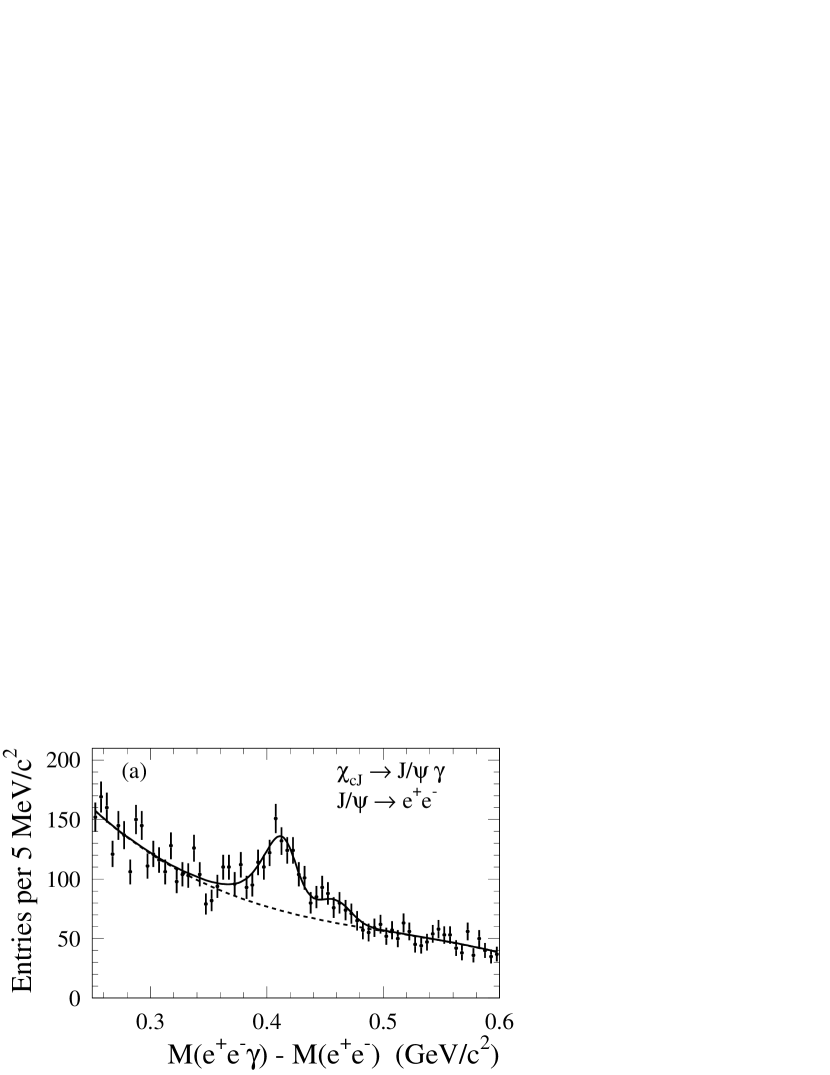
Figure 3: $\chi_{c1}$ and $\chi_{c2}$ candidates reconstructed in the ${J\mskip-3.0mu/\mskip-2.0mu\psi\mskip 2.0mu}\gamma$ final state. Mass difference between the ${J\mskip-3.0mu/\mskip-2.0mu\psi\mskip 2.0mu}\gamma$ and ${J\mskip-3.0mu/\mskip-2.0mu\psi\mskip 2.0mu}$ candidates when the ${J\mskip-3.0mu/\mskip-2.0mu\psi\mskip 2.0mu}$ is reconstructed in the (a) $e^{+}e^{-}$ and (b) $\mu^{+}\mu^{-}$ final states.

Equation 4 is used to determine inclusive $B\rightarrow\chi_{c1}X$ and $B\rightarrow\chi_{c2}X$ branching fractions separately for ${{J\mskip-3.0mu/\mskip-2.0mu\psi\mskip 2.0mu}\rightarrow e^{+}e^{-}}$ and ${{J\mskip-3.0mu/\mskip-2.0mu\psi\mskip 2.0mu}\rightarrow\mu^{+}\mu^{-}}$. In this case, ${\cal B}_{c}={\cal B}(\chi_{cJ}\rightarrow{J\mskip-3.0mu/\mskip-2.0mu\psi\mskip 2.0mu}\gamma)\cdot{\cal B}({J\mskip-3.0mu/\mskip-2.0mu\psi\mskip 2.0mu}\rightarrow\ell^{+}\ell^{-})$, where $\chi_{cJ}$ is $\chi_{c1}$ or $\chi_{c2}$ and $\ell$ is $e$ or $\mu$. Table 1 summarizes the yields, efficiencies, uncertainties and branching fraction products ${\cal B}(B\rightarrow\chi_{cJ}X)\cdot{\cal B}(\chi_{cJ}\rightarrow{J\mskip-3.0mu/\mskip-2.0mu\psi\mskip 2.0mu}\gamma)\cdot{\cal B}({J\mskip-3.0mu/\mskip-2.0mu\psi\mskip 2.0mu}\rightarrow\ell^{+}\ell^{-})$. The 4.5% ($\chi_{c1}$) and 5.3% ($\chi_{c2}$) systematic errors common to both $e^{+}e^{-}$ and $\mu^{+}\mu^{-}$ include photon reconstruction in addition to the ${J\mskip-3.0mu/\mskip-2.0mu\psi\mskip 2.0mu}$ reconstruction items.

As with the ${J\mskip-3.0mu/\mskip-2.0mu\psi\mskip 2.0mu}$, the inclusive $B$ branching fractions to the $\chi_{c1}$ and $\chi_{c2}$ are calculated separately using the ${{J\mskip-3.0mu/\mskip-2.0mu\psi\mskip 2.0mu}\rightarrow e^{+}e^{-}}$ and ${{J\mskip-3.0mu/\mskip-2.0mu\psi\mskip 2.0mu}\rightarrow\mu^{+}\mu^{-}}$ decays. The two values are then combined, distinguishing uncertainties common to both from those unique to a single final state.

The branching fraction obtained for the $\chi_{c2}$ is comparable to that for the $\chi_{c1}$ and is summarized in Table 2. This result is consistent with a prediction from a color octet calculation ref:bodwinc2 , and is in contrast to the expectation of a null result in a factorization calculation ref:kuhn .

VII $\psi{(2S)}$ Production

The reconstruction of the $\psi{(2S)}$ in the $\ell^{+}\ell^{-}$ final state is very similar to the ${J\mskip-3.0mu/\mskip-2.0mu\psi\mskip 2.0mu}$ reconstruction outlined in Sec. V.1, with the ${p^{*}}$ requirement tightened to ${p^{*}}<1.6$${\mathrm{\,Ge\kern-1.00006ptV\!/}c}$. Figure 4 shows the resulting candidate mass distribution. A fit to extract the number of mesons in each plot is performed as for the ${J\mskip-3.0mu/\mskip-2.0mu\psi\mskip 2.0mu}$, but with the resolution and bremsstrahlung parameters fixed to the values found in the higher-statistics ${J\mskip-3.0mu/\mskip-2.0mu\psi\mskip 2.0mu}$ channels. These parameters are varied according to their uncertainties as one contribution to the systematic error on the fit; the remaining contributions are determined as for the ${J\mskip-3.0mu/\mskip-2.0mu\psi\mskip 2.0mu}$.

These data are used to calculate the branching fraction product ${\cal B}(B\rightarrow\psi{(2S)}X)\cdot{\cal B}(\psi{(2S)}\rightarrow\ell^{+}\ell^{-})$, and are later used in the determination of the ${p^{*}}$ distribution of $\psi{(2S)}$ mesons produced in $B$ decay. However, the extraction of the $B\rightarrow\psi{(2S)}X$ branching fraction requires the use of $\psi{(2S)}\rightarrow e^{+}e^{-}$ and $\psi{(2S)}\rightarrow\mu^{+}\mu^{-}$ branching fractions. Since this same data set has previously been used to measure these branching fractions ref:psi2s , we do not use $\psi{(2S)}\rightarrow\ell^{+}\ell^{-}$ events to find ${\cal B}(B\rightarrow\psi{(2S)}X)$.

Figure 4: Mass distribution of $\psi{(2S)}$ candidates reconstructed in the (a) $e^{+}e^{-}$ and (b) $\mu^{+}\mu^{-}$ final states.

Instead, we use $\psi{(2S)}\rightarrow{J\mskip-3.0mu/\mskip-2.0mu\psi\mskip 2.0mu}\pi^{+}\pi^{-}$ for this purpose. The reconstruction of a $\psi{(2S)}$ candidate in this final state starts with a ${J\mskip-3.0mu/\mskip-2.0mu\psi\mskip 2.0mu}$ candidate satisfying the tighter mass constraints used in $\chi_{cJ}$ reconstruction. All charged particles, including those failing the “good-track” criteria, are assumed to be pion candidates. The pion pair is required to be oppositely charged and to have a mass, calculated by four-vector addition, in the range 0.45 to 0.60${\mathrm{\,Ge\kern-1.00006ptV\!/}c^{2}}$. The mass distribution from simulation is compared to the measured ref:bes distribution to obtain a systematic error of 0.5% on reconstruction efficiency. Finally, the ${p^{*}}$ of the $\psi{(2S)}$ candidate is required to be less than 1.6${\mathrm{\,Ge\kern-1.00006ptV\!/}c}$.

Figure 5 displays the mass difference between the $\psi{(2S)}$ and the ${J\mskip-3.0mu/\mskip-2.0mu\psi\mskip 2.0mu}$ candidates separately for ${{J\mskip-3.0mu/\mskip-2.0mu\psi\mskip 2.0mu}\rightarrow e^{+}e^{-}}$ and ${{J\mskip-3.0mu/\mskip-2.0mu\psi\mskip 2.0mu}\rightarrow\mu^{+}\mu^{-}}$. As for the other final states, the distributions are fit to obtain the number of mesons. The resolution smearing parameters are not required to be the same for the two plots, but are consistent: $1.5\pm 0.8$${\mathrm{\,Me\kern-1.00006ptV\!/}c^{2}}$ ($e^{+}e^{-}$) and $1.8\pm 0.5$${\mathrm{\,Me\kern-1.00006ptV\!/}c^{2}}$ ($\mu^{+}\mu^{-}$). The secondary branching fractions in Eq. 4 are in this case ${\cal B}_{c}={\cal B}(\psi{(2S)}\rightarrow{J\mskip-3.0mu/\mskip-2.0mu\psi\mskip 2.0mu}\pi^{+}\pi^{-})\cdot{\cal B}({J\mskip-3.0mu/\mskip-2.0mu\psi\mskip 2.0mu}\rightarrow\ell^{+}\ell^{-})$.

Figure 5: $\psi{(2S)}$ candidates reconstructed in the ${J\mskip-3.0mu/\mskip-2.0mu\psi\mskip 2.0mu}\pi^{+}\pi^{-}$ final state. Mass difference between the ${J\mskip-3.0mu/\mskip-2.0mu\psi\mskip 2.0mu}\pi^{+}\pi^{-}$ and ${J\mskip-3.0mu/\mskip-2.0mu\psi\mskip 2.0mu}$ candidates when the ${J\mskip-3.0mu/\mskip-2.0mu\psi\mskip 2.0mu}$ is reconstructed in the (a) $e^{+}e^{-}$ and (b) $\mu^{+}\mu^{-}$ final states.

VIII Direct Branching Fractions

To obtain the branching fraction for ${J\mskip-3.0mu/\mskip-2.0mu\psi\mskip 2.0mu}$ mesons produced directly in the decay of $B$ mesons, we subtract the feeddown contributions to the inclusive branching fraction due to the decay of $\chi_{c1}$, $\chi_{c2}$, and $\psi{(2S)}$ mesons. For the $\chi_{c1}$ and $\chi_{c2}$, the feeddown branching fraction is ${\cal B}(B\rightarrow\chi_{cJ}X)\cdot{\cal B}(\chi_{cJ}\rightarrow{J\mskip-3.0mu/\mskip-2.0mu\psi\mskip 2.0mu}\gamma)$, while for the $\psi{(2S)}$, it is ${\cal B}(B\rightarrow\psi{(2S)}X)\cdot{\cal B}(\psi{(2S)}\rightarrow{J\mskip-3.0mu/\mskip-2.0mu\psi\mskip 2.0mu}X)$.

Similarly, the feeddown from the $\psi{(2S)}$ to the $\chi_{c1}$ and $\chi_{c2}$ is ${\cal B}(B\rightarrow\psi{(2S)}X)\cdot{\cal B}(\psi{(2S)}\rightarrow\chi_{cJ}\gamma)$.

Note that a number of uncertainties are common to both the inclusive and feeddown components, including track quality and particle identification criteria, ${\cal B}(\chi_{c1}\rightarrow{J\mskip-3.0mu/\mskip-2.0mu\psi\mskip 2.0mu}\gamma)$, and ${\cal B}(\chi_{c2}\rightarrow{J\mskip-3.0mu/\mskip-2.0mu\psi\mskip 2.0mu}\gamma)$. We use world average values ref:pdg2000 for the $\psi{(2S)}$ branching fractions. The resulting direct branching fractions are summarized in Table 2.

Table 2: Summary of $B$ branching fractions (percent) to charmonium mesons with statistical and systematic uncertainties. The direct branching fraction is also listed, where appropriate. Last column contains the world average values ref:pdg2000 .

Meson	Value	Stat	Sys	World Average
${J\mskip-3.0mu/\mskip-2.0mu\psi\mskip 2.0mu}$	1.057	$\pm 0.012$	$\pm 0.040$	$1.15\pm 0.06$
${J\mskip-3.0mu/\mskip-2.0mu\psi\mskip 2.0mu}$ direct	0.740	$\pm 0.023$	$\pm 0.043$	$0.80\pm 0.08$
$\chi_{c1}$	0.367	$\pm 0.035$	$\pm 0.044$	$0.36\pm 0.05$
$\chi_{c1}$ direct	0.341	$\pm 0.035$	$\pm 0.042$	$0.33\pm 0.05$
$\chi_{c2}$	0.210	$\pm 0.045$	$\pm 0.031$	$0.07\pm 0.04$
$\chi_{c2}$ direct	0.190	$\pm 0.045$	$\pm 0.029$	–
$\psi{(2S)}$	0.297	$\pm 0.020$	$\pm 0.020$	$0.35\pm 0.05$

IX ${p^{*}}$ Distributions

The momentum distributions of charmonium mesons provide an insight into their production mechanisms. Since we do not fully reconstruct the $B$ meson, we cannot determine the meson momentum in the $B$ rest frame and instead use ${p^{*}}$, the value in the $\mathchar 28935\relax{(4S)}$ center-of-mass frame. The difference, due to the motion of the $B$ in the center-of-mass frame, has an rms spread of 0.12${\mathrm{\,Ge\kern-1.00006ptV\!/}c}$.

IX.1 Inclusive ${p^{*}}$ Distributions

To measure the ${p^{*}}$ distributions of ${J\mskip-3.0mu/\mskip-2.0mu\psi\mskip 2.0mu}$, $\chi_{c1}$, $\chi_{c2}$, and $\psi{(2S)}$ mesons produced in $B$ decays, we create mass or mass-difference histograms of on-resonance candidates with ${p^{*}}$ in the desired range. The $e^{+}e^{-}$ and $\mu^{+}\mu^{-}$ final states are again treated separately. The distributions are then fit, with all signal pdf parameters (other than the number of mesons) fixed to the values obtained from the earlier fits. The fits are performed for 100${\mathrm{\,Me\kern-1.00006ptV\!/}c}$ wide ${p^{*}}$ ranges, and in each case the sum of the yields differs from the original fit by fewer than ten events.

In the case of the ${J\mskip-3.0mu/\mskip-2.0mu\psi\mskip 2.0mu}$, we perform similar fits on the off-resonance data and perform a continuum subtraction for each ${p^{*}}$ bin. Since there are no statistically significant off-resonance $\chi_{c1}$, $\chi_{c2}$, or $\psi{(2S)}$ signals, we do not perform a continuum subtraction in these cases.

The yield in each bin is corrected by the reconstruction efficiency obtained from simulated data, which decreases by approximately 10% between 0 and 2${\mathrm{\,Ge\kern-1.00006ptV\!/}c}$. The yield is then multiplied by an overall normalization factor for that particular final state and mode, which adjusts the sum of all bins to the earlier branching fraction measurement. We then perform a weighted average of the two distributions for the ${J\mskip-3.0mu/\mskip-2.0mu\psi\mskip 2.0mu}$, $\chi_{c1}$, or $\chi_{c2}$, or the four distributions for the $\psi{(2S)}$, to obtain the distributions shown in Fig. 6–8. For this purpose, we use the $\psi{(2S)}\rightarrow e^{+}e^{-}$ and $\psi{(2S)}\rightarrow\mu^{+}\mu^{-}$ branching fractions from Ref. ref:psi2s . In all cases, the distributions that are combined are consistent within statistical errors.

Figure 6: $B\rightarrow{J\mskip-3.0mu/\mskip-2.0mu\psi\mskip 2.0mu}X$ branching fraction as a function of ${p^{*}}$.

Figure 7: Branching fraction as a function of ${p^{*}}$ for (a) $B\rightarrow\chi_{c1}X$ and (b) $B\rightarrow\chi_{c2}X$. The distribution includes a small feeddown component from the $\psi{(2S)}$ (solid curve).

Figure 8: $B\rightarrow\psi{(2S)}X$ branching fraction as a function of ${p^{*}}$.

IX.2 Direct ${p^{*}}$ Distributions

The ${J\mskip-3.0mu/\mskip-2.0mu\psi\mskip 2.0mu}$ ${p^{*}}$ distribution (Fig. 6) includes components due to mesons from the decays $\chi_{c1}\rightarrow{J\mskip-3.0mu/\mskip-2.0mu\psi\mskip 2.0mu}\gamma$, $\chi_{c2}\rightarrow{J\mskip-3.0mu/\mskip-2.0mu\psi\mskip 2.0mu}\gamma$, and $\psi{(2S)}\rightarrow{J\mskip-3.0mu/\mskip-2.0mu\psi\mskip 2.0mu}X$. To measure these distributions, we repeat the analysis with the data binned by the ${p^{*}}$ of the ${J\mskip-3.0mu/\mskip-2.0mu\psi\mskip 2.0mu}$  daughter. The resulting ${J\mskip-3.0mu/\mskip-2.0mu\psi\mskip 2.0mu}$ feeddown distributions are presented in Fig. 9.

Note that we are using only the ${J\mskip-3.0mu/\mskip-2.0mu\psi\mskip 2.0mu}\pi^{+}\pi^{-}$ decay mode to obtain the ${J\mskip-3.0mu/\mskip-2.0mu\psi\mskip 2.0mu}$ distribution from $\psi{(2S)}$ decay. In fact, 10.5% of $\psi{(2S)}\rightarrow{J\mskip-3.0mu/\mskip-2.0mu\psi\mskip 2.0mu}X$ decays are modes other than ${J\mskip-3.0mu/\mskip-2.0mu\psi\mskip 2.0mu}\pi\pi$. If we instead use the simulated ${J\mskip-3.0mu/\mskip-2.0mu\psi\mskip 2.0mu}$ distribution for this 10.5%, Fig. 9c changes by no more than a small fraction of the statistical error bar in any bin.

Figure 9: Contributions to the $B\rightarrow{J\mskip-3.0mu/\mskip-2.0mu\psi\mskip 2.0mu}X$ branching fraction as a function of ${p^{*}}$ due to feeddown from (a) $\chi_{c1}$, (b) $\chi_{c2}$   and (c) $\psi{(2S)}$ mesons.

Subtracting these three components from the inclusive ${J\mskip-3.0mu/\mskip-2.0mu\psi\mskip 2.0mu}$  distribution in Fig. 6 leaves the contribution due to the ${J\mskip-3.0mu/\mskip-2.0mu\psi\mskip 2.0mu}$ mesons produced directly in $B$ decay (Fig. 10).

The superimposed histogram is a calculation of the expected distribution, which includes color octet and color singlet components. We use a recent NRQCD calculation ref:benekep for the color octet component. The authors attribute the singlet component to ${J\mskip-3.0mu/\mskip-2.0mu\psi\mskip 2.0mu}K^{(*)}$ production, which we obtain from simulation. The two are normalized to obtain the best fit to our data. Possible sources of the apparent excess at low momentum are an intrinsic charm component of the $B$ ref:hou , the production, together with the ${J\mskip-3.0mu/\mskip-2.0mu\psi\mskip 2.0mu}$, of baryons ref:brodsky , or an $s{\overline{d}}g$ hybrid ref:eilam .

The small feeddown contribution to $\chi_{c1}$ and $\chi_{c2}$ from $\psi{(2S)}$ decay is calculated by simulation and is shown in Fig. 7.

Figure 10: ${p^{*}}$ of ${J\mskip-3.0mu/\mskip-2.0mu\psi\mskip 2.0mu}$ mesons produced directly in $B$ decays (points). The histogram is the sum of the color-octet component from a recent NRQCD calculation ref:benekep (dashed line) and the color-singlet ${J\mskip-3.0mu/\mskip-2.0mu\psi\mskip 2.0mu}K^{(*)}$ component from simulation (dotted line).

X ${J\mskip-3.0mu/\mskip-2.0mu\psi\mskip 2.0mu}$ Helicity

The helicity $\theta_{H}$ of a ${J\mskip-3.0mu/\mskip-2.0mu\psi\mskip 2.0mu}\rightarrow\ell^{+}\ell^{-}$ candidate is the angle, measured in the ${J\mskip-3.0mu/\mskip-2.0mu\psi\mskip 2.0mu}$ rest frame, between the positively charged lepton and the flight direction of the ${J\mskip-3.0mu/\mskip-2.0mu\psi\mskip 2.0mu}$ in the $\mathchar 28935\relax{(4S)}$  center-of-mass frame. A more natural definition would use the $B$ rest frame, but it cannot be determined in this analysis. Simulation indicates that the rms spread of the difference between the two definitions is 0.085 in ${\cos\theta_{H}}$.

Figure 11: Helicity of ${J\mskip-3.0mu/\mskip-2.0mu\psi\mskip 2.0mu}$ mesons produced in $B$ decay with ${p^{*}}>1.1$ ${\mathrm{\,Ge\kern-1.00006ptV\!/}c}$ (dots) and ${p^{*}}<1.1$ ${\mathrm{\,Ge\kern-1.00006ptV\!/}c}$ (open squares).

X.1 Inclusive Helicity Distribution

We proceed as for the ${J\mskip-3.0mu/\mskip-2.0mu\psi\mskip 2.0mu}$ ${p^{*}}$ distribution, with data categorized into ranges of width 0.1 in ${\cos\theta_{H}}$ for two different momentum ranges, which we choose as ${p^{*}}<1.1$${\mathrm{\,Ge\kern-1.00006ptV\!/}c}$ and $1.1<{p^{*}}<2.0$${\mathrm{\,Ge\kern-1.00006ptV\!/}c}$. We fit the on- and off-resonance mass distributions to obtain yields in each bin and perform a continuum subtraction. We correct using the reconstruction efficiency obtained from simulation for that range, although we observe little dependence of efficiency on helicity. We then apply separate normalization factors to the $e^{+}e^{-}$ and $\mu^{+}\mu^{-}$ data such that the total branching fraction (summed over the two ${p^{*}}$ ranges) agrees with the value obtained earlier for that mode. The distributions from $e^{+}e^{-}$ and $\mu^{+}\mu^{-}$  are consistent and are averaged to obtain the helicity distributions for each of the two ${p^{*}}$ ranges (Fig. 11).

We fit each distribution with a function $1+\alpha\cdot\cos^{2}\theta_{H}$ to obtain the polarization $\alpha$, where $\alpha=0$ indicates the sample is unpolarized, $\alpha=1$ transversely polarized, and $\alpha=-1$ longitudinally polarized. The high ${p^{*}}$ region, which includes the two-body $B$ decays, is more highly polarized, $\alpha=-0.592\pm 0.032$, than the lower ${p^{*}}$ region, $\alpha=-0.196\pm 0.044$.

We assign a systematic error of 0.008 to these polarizations by instead considering the reconstruction efficiency to be independent of helicity.

Figure 12: Helicity distribution of ${J\mskip-3.0mu/\mskip-2.0mu\psi\mskip 2.0mu}$ mesons produced in the decay of (a) $\chi_{c1}$, (b) $\chi_{c2}$, and (c) $\psi{(2S)}$ mesons.

X.2 Direct ${J\mskip-3.0mu/\mskip-2.0mu\psi\mskip 2.0mu}$ Helicity

We determine the helicity distributions of ${J\mskip-3.0mu/\mskip-2.0mu\psi\mskip 2.0mu}$ mesons produced in the decay of $\chi_{c1}$, $\chi_{c2}$, and $\psi{(2S)}$ in the same way we calculate the ${p^{*}}$ feeddown. Because of the limited statistics of these samples, we combine the two momentum regions used in the inclusive analysis. The resulting feeddown helicity distributions are shown together with the polarization fits in Fig. 12. We subtract these from the sum of the two distributions in Fig. 11 to obtain the helicity distribution for the ${J\mskip-3.0mu/\mskip-2.0mu\psi\mskip 2.0mu}$ produced directly in $B$ decay (Fig. 13). The polarization, $\alpha=-0.46\pm 0.06$, is slightly out of the range $-0.33$ to 0.05 predicted by an NRQCD calculation ref:fleming , but other authors have argued ref:ma that relativistic corrections reduce the reliability of the calculation. The systematic uncertainty of 0.008 obtained above is small compared to the statistical error. This result is difficult to compare directly with that from CDF ref:cdfpol , due to the different mixture of $b$ mesons and baryons, and the distinction between the effective helicity calculated there and the true helicity.

Figure 13: Helicity distribution of ${J\mskip-3.0mu/\mskip-2.0mu\psi\mskip 2.0mu}$ mesons produced directly in the decay of $B$ mesons.

XI Summary

We have reported new measurements of $B$ meson decays to final states including charmonium mesons, which are summarized in Table 2. We have presented a number of momentum distributions. The distributions of the feeddown ${J\mskip-3.0mu/\mskip-2.0mu\psi\mskip 2.0mu}$  daughters of the $\chi_{c1}$, $\chi_{c2}$, and $\psi{(2S)}$ have not previously been measured, and allow us to more accurately determine the distribution for ${J\mskip-3.0mu/\mskip-2.0mu\psi\mskip 2.0mu}$ mesons produced directly in $B$ decay. The direct ${J\mskip-3.0mu/\mskip-2.0mu\psi\mskip 2.0mu}$ distribution is compared to a recent NRQCD calculation and appears to indicate an excess at low momentum.

The ${J\mskip-3.0mu/\mskip-2.0mu\psi\mskip 2.0mu}$ helicity distribution, which has also has not previously been published, indicates that the polarization of direct ${J\mskip-3.0mu/\mskip-2.0mu\psi\mskip 2.0mu}$  mesons is slightly out of the range predicted by an NRQCD calculation.

We are grateful for the excellent luminosity and machine conditions provided by our PEP-II colleagues, and for the substantial dedicated effort from the computing organizations that support BABAR. The collaborating institutions wish to thank SLAC for its support and kind hospitality. This work is supported by DOE and NSF (USA), NSERC (Canada), IHEP (China), CEA and CNRS-IN2P3 (France), BMBF and DFG (Germany), INFN (Italy), NFR (Norway), MIST (Russia), and PPARC (United Kingdom). Individuals have received support from the A. P. Sloan Foundation, Research Corporation, and Alexander von Humboldt Foundation.

References

(1)
G. T. Bodwin, E. Braaten, and G. P. Lepage, Phys. Rev. D 51, 1125
(1995); Erratum 55, 5853 (1997); M. Beneke, F. Maltoni, and
I. Z. Rothstein, Phys. Rev. D 59, 054003 (1999).
(2)
E. Braaten and S. Fleming, Phys. Rev. Lett. 74, 3327 (1995); M. Cacciari,
M. Greco, M.L. Mangano, and A. Petrelli, Phys. Lett. B 356, 553 (1995).
(3)
CDF Collaboration, F. Abe et al., Phys. Rev. Lett. 69, 3704 (1992);
79, 572 (1997); 79, 578 (1997). D0 Collaboration, S. Abachi et al., Phys. Lett. B 370, 239 (1996).
(4)
A. K. Leibovich, Nucl. Phys. Proc. Suppl. 93, 182 (2001); G. A. Schuler,
Eur. Phys. Jour. C 8, 273 (1999).
(5)
CLEO Collaboration, R. Balest et al., Phys. Rev. D 52, 2661 (1995);
S. Chen et al., Phys. Rev. D 63, 031102 (2001).
(6)
Belle Collaboration, K. Abe et al., Phys. Rev. Lett. 89, 011803 (2002).
(7)BABAR Collaboration, B. Aubert et al.,
Nucl. Instr. and Methods A479, 1 (2002).
(8)
“GEANT Detector Description and Simulation Tool”, Version 3.21, CERN
Program Library Long Writeup W5013 (1994).
(9)
G. C. Fox and S. Wolfram, Phys. Rev. Lett. 41, 1581 (1978).
(10)
T. Sjostrand, Computer Physics Commun. 82 (1994) 74.
(11)
A. Drescher et al., Nucl. Instr. and Methods A237, 464 (1985). , where the
crystals in the EMC cluster are ranked in order of energy deposited in
that crystal, ,
and is the average distance between crystal
centers. is the distance between crystal and the cluster
centroid calculated from an energy-weighted average of the
crystals.
(12)
R. Sinkus and T. Voss, Nucl. Instr. and Methods A391, 360 (1997).
The Zernike moment is calculated using the energy and
location of crystals with respect to the shower
centroid. The location
is defined in a cylindrical coordinate system with the axis
running from
the beam spot to the centroid, where and . , where the sum includes only crystals with
, and is the total energy in the cluster. The Zernike
functions are
, with and
even. Studies indicate that provides good
separation between hadronic and electromagnetic showers when used in
conjunction with LAT.
(13)BABAR Collaboration, B. Aubert et al., Phys. Rev. Lett. 87, 162002 (2001);
Belle Collaboration, K. Abe et al., Phys. Rev. Lett. 88, 052001 (2002).
(14)
E. Barberio, B. van Eijk, and Z. Was, Comput. Phys. Commun. 66, 115 (1991).
(15)
Particle Data Group, K. Hagiwara et al., Phys. Rev. D 66, 010001 (2002).
(16)
G.T. Bodwin, E. Braaten, T.C. Yuan, and G.P. Lepage,
Phys. Rev. D 46, 3703 (1992).
(17)
J. H. Kühn, S. Nussinov, and R. Rückl, Z. Phys. C
5, 117 (1980).
(18)BABAR Collaboration, B. Aubert et al., Phys. Rev. D 65, 031101 (2002).
(19)
BES Collaboration, J. Z. Bai et al., Phys. Rev. D 62, 032002 (2000).
(20)
M. Beneke, G.A. Schuler, and S. Wolf, Phys. Rev. D 62, 034004 (2000).
Curve is from Fig. 5, , , and
.
(21)
C.-H.V. Chang and W.-S. Hou, Phys. Rev. D 64, 071501 (2001).
(22)
S.J. Brodsky and F.S. Navarra, Phys. Lett. B 411, 152 (1997).
(23)
G. Eilam, M. Ladisa, and Y.-D. Yang, Phys. Rev. D 65, 037504 (2002).
(24)
S. Fleming et al., Phys. Rev. D 55, 4098 (1997).
(25)
J. P. Ma, Phys. Rev. D 62, 054012 (2000).
(26)
CDF Collaboration, T. Affolder et al., Phys. Rev. Lett. 85, 2886 (2000).