The BABAR Collaboration

July 24, 2002

We present preliminary results from a search for the rare, flavor-changing neutral current decays $B\rightarrow K\ell^{+}\ell^{-}$ and $B\rightarrow K^{*}\ell^{+}\ell^{-}$, where $\ell^{+}\ell^{-}$ is either an $e^{+}e^{-}$ or $\mu^{+}\mu^{-}$ pair. The data sample comprises $(84.4\pm 0.9)\times 10^{6}$ $\mathchar 28935\relax(4S)\rightarrow B\kern 1.79993pt\overline{\kern-1.79993ptB}{}$ decays (77.8 fb^-1) collected with the BABAR detector at the PEP-II $B$ Factory. For $B\rightarrow K\ell^{+}\ell^{-}$, we observe a signal with estimated significance of $4.4\sigma$ and obtain ${\mathcal{B}}(B\rightarrow K\ell^{+}\ell^{-})=(0.78^{+0.24+0.11}_{-0.20-0.18})\times 10^{-6}$ (averaged over $\ell=e$ and $\mu$). For $B\rightarrow K^{*}\ell^{+}\ell^{-}$, we observe an excess of events over background with estimated significance of $2.8\sigma$. We obtain ${\mathcal{B}}(B\rightarrow K^{*}\ell^{+}\ell^{-})=(1.68^{+0.68}_{-0.58}\pm 0.28)\times 10^{-6}$ and the 90% C.L. upper limit ${\mathcal{B}}(B\rightarrow K^{*}\ell^{+}\ell^{-})<3.0\times 10^{-6}$.

1 Introduction

The flavor-changing neutral current decays $B\rightarrow K\ell^{+}\ell^{-}$ and $B\rightarrow K^{*}(892)\ell^{+}\ell^{-}$, where $\ell^{\pm}$ is a charged lepton, are highly suppressed in the Standard Model, with branching fractions predicted to be of order $10^{-7}-10^{-6}$ [1, 2, 3]. The dominant contributions arise at one-loop level and include both electroweak penguin and box diagrams. Besides probing Standard Model loop effects, these rare decays are important because their rates and kinematic distributions are sensitive to new, heavy particles—such as those predicted by supersymmetric models—that can appear virtually in the loops [1, 2, 3].

Searches for $B\rightarrow K^{(*)}\ell^{+}\ell^{-}$ decays have been performed by BABAR [4], Belle [5], CDF [6], and CLEO [7]. Using a sample of 29 fb^-1, the Belle Collaboration has observed a signal for the decay $B\rightarrow K\ell^{+}\ell^{-}$ with branching fraction ${\cal B}(B\rightarrow K\ell^{+}\ell^{-})=(0.75^{+0.25}_{-0.21}\pm 0.09)\times 10^{-6}$, averaged over electron and muon modes. The recently published BABAR [4] result was based on a 20.7 fb^-1 sample and yielded the 90% C.L. upper limits ${\cal B}(B\rightarrow K\ell^{+}\ell^{-})<0.51\times 10^{-6}$ and ${\cal B}(B\rightarrow K^{*}\ell^{+}\ell^{-})<3.1\times 10^{-6}$. In the present study, we update our result with a total sample that is nearly four times larger than that used in the original BABAR analysis.

We search for the following decays: $B^{+}\rightarrow K^{+}\ell^{+}\ell^{-}$, $B^{0}\rightarrow K_{S}^{0}\ell^{+}\ell^{-}$, $B^{+}\rightarrow K^{*+}\ell^{+}\ell^{-}$, and $B^{0}\rightarrow K^{*0}\ell^{+}\ell^{-}$, where $K^{*0}\rightarrow K^{+}\pi^{-}$, $K^{*+}\rightarrow K_{S}^{0}\pi^{+}$, $K_{S}^{0}\rightarrow\pi^{+}\pi^{-}$, and $\ell$ is either an $e$ or $\mu$. Throughout this paper, charge-conjugate modes are implied.

2 Theoretical predictions

The Standard Model processes for $B\rightarrow K^{(*)}\ell^{+}\ell^{-}$ include three contributions: the electromagnetic (EM) and $Z$ penguin diagrams, and the $W^{+}W^{-}$ box diagrams (Fig. 1). Evidence for the EM penguin amplitude was first obtained by the CLEO experiment from the observation of the exclusive decay $B\rightarrow K^{*}\gamma$ and later from the inclusive process $B\rightarrow X_{s}\gamma$, where $X_{s}$ is any hadronic system with strangeness [8, 9]. Since then, several experiments have observed these decays, and the Particle Data Group [10] calculates the world averages ${\cal B}(B^{0}\rightarrow K^{*0}\gamma)=(4.3\pm 0.4)\times 10^{-5}$ and ${\cal B}(B\rightarrow X_{s}\gamma)=(3.3\pm 0.4)\times 10^{-4}$.

Figure 1: Standard Model diagrams for the decays $B\rightarrow K^{(*)}\ell^{+}\ell^{-}$.

The Standard Model rates for $B\rightarrow K^{*}\ell^{+}\ell^{-}$ and $B\rightarrow X_{s}\ell^{+}\ell^{-}$ are expected to be 25–80 times smaller than those for $B\rightarrow K^{*}\gamma$ and $B\rightarrow X_{s}\gamma$. For example, Ali et al. predict [3] ${\cal B}(B\rightarrow X_{s}e^{+}e^{-})=(6.89\pm 1.01)\times 10^{-6}$ and ${\cal B}(B\rightarrow X_{s}\mu^{+}\mu^{-})=(4.15\pm 0.70)\times 10^{-6}$ for the inclusive branching fractions. Exclusive final states have larger theoretical uncertainties but are experimentally more accessible. Ali et al. [3] predict ${\cal B}(B\rightarrow K\ell^{+}\ell^{-})=(0.35\pm 0.12)\times 10^{-6}$ for both $e^{+}e^{-}$ and $\mu^{+}\mu^{-}$ final states, ${\cal B}(B\rightarrow K^{*}e^{+}e^{-})=(1.58\pm 0.49)\times 10^{-6}$, and ${\cal B}(B\rightarrow K^{*}\mu^{+}\mu^{-})=(1.19\pm 0.39)\times 10^{-6}$.

Figure 2 shows the predicted rates as a function of $q^{2}\equiv m_{\ell^{+}\ell^{-}}^{2}$ for a number of theoretical models. The $B\rightarrow K\ell^{+}\ell^{-}$ modes display a falloff in the rate from low values of $q^{2}$ (fast recoil kaon) to high values (slow recoil kaon). (Although $B\rightarrow K\gamma$ is forbidden by angular momentum conservation, $B\rightarrow K\ell^{+}\ell^{-}$ is allowed since $q^{2}>0$.) The $q^{2}$ distributions for $B\rightarrow K^{*}\ell^{+}\ell^{-}$ behave quite differently, with large enhancements at low $q^{2}$, but otherwise with the maximum rate at some intermediate $q^{2}$ value. The low $q^{2}$ enhancements are due to the EM penguin amplitude, which has a pole at $q^{2}=0$, strongly enhancing $B\rightarrow K^{*}e^{+}e^{-}$ and, to a lesser extent, $B\rightarrow K^{*}\mu^{+}\mu^{-}$. As a consequence, most Standard-Model-based predictions give a higher rate for $B\rightarrow K^{*}e^{+}e^{-}$ than for $B\rightarrow K^{*}\mu^{+}\mu^{-}$. At values of $q^{2}$ above this pole region, the contributions from the $Z$ penguin and the $W^{+}W^{-}$ box diagram become very important.

Figure 2: Model predictions [1] for the decay rate as a function of $q^{2}$ for (a) $B\rightarrow Ke^{+}e^{-}$ (b) $B\rightarrow K\mu^{+}\mu^{-}$ (c) $B\rightarrow K^{*}e^{+}e^{-}$ and (d) $B\rightarrow K^{*}\mu^{+}\mu^{-}$. The solid histogram is based on the light cone QCD sum rules model of Ali et al., the dashed histogram on the QCD sum rules model of Colangelo et al., and the dot-dashed histogram on the quark model of Melikhov, Nikitin, and Simula. The distributions are normalized to the same area, so that any differences in the overall rates are not shown.

While the $B\rightarrow K^{(*)}\ell^{+}\ell^{-}$ decays are rarer than the pure EM penguin processes, they have sensitivity to three Wilson coefficients $C_{7}$, $C_{9}$, and $C_{10}$ in the Operator Product Expansion [1], whereas the $b\rightarrow s\gamma$ rate is sensitive mainly to the magnitude of a single Wilson coefficient, $C_{7}$. New physics could, for example, change the sign of $C_{7}$ in $B\rightarrow K^{*}\ell^{+}\ell^{-}$; the resulting modification of the interference terms with the other amplitudes could enhance the rate by a factor of two over the Standard Model prediction.

Measurements of the kinematic distributions in $B\rightarrow K^{*}\ell^{+}\ell^{-}$ decays will eventually provide a probe of new physics with less theoretical uncertainty than the decay rates. Certain features of the lepton angular distribution as a function of $q^{2}$ can be predicted reliably and can be dramatically modified by new physics. In particular, the lepton forward-backward asymmetry in the dilepton rest frame is predicted to become zero at a particular value of $q^{2}$ in the Standard Model, but the sign of the asymmetry and the location of the zero can be modified by new physics. The study of these angular distributions will require very large data samples and will be investigated by future experiments, including those at the LHC.

3 The BABAR detector and data sample

The data used in the analysis were collected with the BABAR detector at the PEP-II asymmetric energy $e^{+}e^{-}$ storage ring at the Stanford Linear Accelerator Center. We analyze the data taken in the 1999–2002 runs, consisting of a 77.8 $\mbox{\,fb}^{-1}$ sample accumulated on the $\mathchar 28935\relax(4S)$ resonance, as well as 9.6 $\mbox{\,fb}^{-1}$ taken at a center-of-mass energy 40 MeV below the $\mathchar 28935\relax(4S)$ resonance peak to obtain a pure continuum sample. Continuum events include non-resonant $e^{+}e^{-}\rightarrow q\overline{q}$ production, where $q=u$, $d$, $s$, or $c$, as well as two-photon and $\tau^{+}\tau^{-}$ events. The on-resonance sample contains $(84.4\pm 0.9)\times 10^{6}$ $\mathchar 28935\relax(4S)\rightarrow B\kern 1.79993pt\overline{\kern-1.79993ptB}{}$ events.

The BABAR detector is described in detail elsewhere [11]. Of particular importance for this analysis are the charged-particle tracking system and the detectors used for particle identification. At radii between about 3 cm and 14 cm, charged tracks are measured in a five-layer silicon vertex tracker (SVT). Tracking beyond the SVT is provided by the drift chamber, which extends in radius from 23.6 to 80.9 cm and provides up to 40 track-measurement points. Just outside the drift chamber is the DIRC, a Cherenkov ring-imaging particle identification system. The DIRC provides charged particle velocity information through the measurement of the Cherenkov light cone opening angle. Cherenkov light is produced by charged particles as they pass through an array of 144 five-meter-long fused silica quartz bars. The Cherenkov light is transmitted to the instrumented end of the bars by total internal reflection, preserving the information on the angle of the light emission with respect to the track direction. The DIRC is used for kaon identification in this analysis and is essential to our background rejection. Electrons are identified using an electromagnetic calorimeter comprising 6580 thallium-doped CsI crystals. These systems are mounted inside a 1.5 T solenoidal superconducting magnet to provide momentum measurement in the charged particle tracking systems. Muons are identified using the Instrumented Flux Return (IFR), in which resistive plate chambers (RPCs) are interleaved with the iron plates of the magnet flux return.

4 Analysis overview

The most obvious analysis challenge is that in each of the eight signal channels there are background processes with identical final-state particles that proceed through charmonium resonances. For example, the decay $B\rightarrow K^{+}\ell^{+}\ell^{-}$ has backgrounds from $B\rightarrow J/\psi(\rightarrow\ell^{+}\ell^{-})K^{+}$ and $B\rightarrow\psi(2S)(\rightarrow\ell^{+}\ell^{-})K^{+}$ that must be carefully understood and vetoed. These backgrounds are particularly difficult in the electron channels, where bremsstrahlung in detector material can easily cause the dilepton mass to fall well below that of the mass of the charmonium resonance. On the other hand, these backgrounds provide nearly ideal control samples for each channel, allowing us to make data vs. Monte Carlo comparisons and checks of selection criteria efficiencies in a way that carries over almost directly to the signal processes. Before searching for a signal in any newly acquired data sample, we validate our analysis by comprehensively studying the yields and shapes of distributions in the charmonium control samples. Although these processes have a narrow distribution in $q^{2}$, they still allow us to confirm that the lepton identification efficiencies used in the Monte Carlo simulations are valid over a broad range of momenta. We have therefore studied the charmonium control samples in detail, not only to design our vetoes, but also to establish signal shape parameters and to verify Monte Carlo predictions of signal efficiencies.

The most important non-charmonium background contributions are from $B\overline{B}$ backgrounds with either two real leptons or one real lepton and one hadron misidentified as a lepton (usually as a muon); continuum processes, especially $c\overline{c}$ events with a pair of $D\rightarrow K^{(*)}\ell^{+}\nu$ decays or events with hadrons faking leptons; and small, but potentially very important contributions from a number of $B$ decay modes with similar topology to the signal, such as $B^{+}\rightarrow D^{0}\pi^{+}$ with $D^{0}\rightarrow K^{-}\pi^{+}$, in which hadrons misidentified as leptons can create a false signal. Another example of a signal-like background is $B\rightarrow K^{*}\gamma$ followed by conversion of the photon into $e^{+}e^{-}$ in the detector material. This process is distinct from the decay $B\rightarrow K^{*}e^{+}e^{-}$ at low $q^{2}$, where the photon undergoes internal conversion. While no single such background is large, it is important to establish that the sum of many processes with very small contributions does not produce a significant number of peaking background events.

In the $B\rightarrow K\ell^{+}\ell^{-}$ modes, the dominant background is from continuum events. Much of this background can be suppressed using event shape variables that discriminate between the jet-like topology of continuum events and the much more spherical topology of signal (and other $B\overline{B}$ events). In $B\rightarrow K^{*}\ell^{+}\ell^{-}$ channels, the $B\overline{B}$ background is substantially larger than that from the continuum. Much of the $B\overline{B}$ background is due to pairs of primary semileptonic decays from the $B$ and $\overline{B}$ mesons. Such events are characterized by large amounts of missing energy associated with the two neutrinos. We have constructed two main analysis variables, one for $B\overline{B}$ rejection ($B$ likelihood) and one for continuum-background rejection (Fisher discriminant). Each of these variables combines information from several kinematic quantities.

To prevent bias in the analysis, we optimize the event-selection criteria using (1) Monte Carlo samples both signal and background, (2) the off-resonance data, and (3) a “large sideband” region in the data that is outside of the fit region (defined below). Signal efficiencies were determined using the model of Ali et al. [1], although a set of other models [1] was used to estimate a systematic uncertainty on the efficiencies due to model dependence. None of our models for the signal efficiency include small effects arising from interference between the electroweak penguin amplitudes and the amplitudes for the decays involving charmonium intermediate states. The interference is constructive on the lower side of the $J/\psi$ and $\psi(2S)$ charmonium resonance masses but is destructive on the upper side. The effect of this interference on our yields is also suppressed by the charmonium vetoes.

After event selection, we perform a two-dimensional unbinned maximimum likelihood fit to the joint distribution in

$$m_{\rm ES} = \sqrt{E_{\rm b}^{*2}-(\sum_{i}{\bf p}^{*}_{i})^{2}}$$

$$\Delta E = \sum_{i}\sqrt{m_{i}^{2}+{\bf p}_{i}^{*2}}-E_{\rm b}^{*},$$

where $E_{\rm b}^{*}$ is the beam energy in the $e^{+}e^{-}$ rest (CM) frame, ${\bf p}_{i}^{*}$ is the CM momentum of daughter particle $i$ of the $B$ meson candidate, and $m_{i}$ is the mass hypothesis for particle $i$. For signal events, $m_{\rm ES}$ peaks at the $B$ meson mass with a resolution of about 2.5 MeV$/c^{2}$ and $\Delta E$ peaks near zero, indicating that the candidate system of particles has total energy consistent with the beam energy in the CM frame.

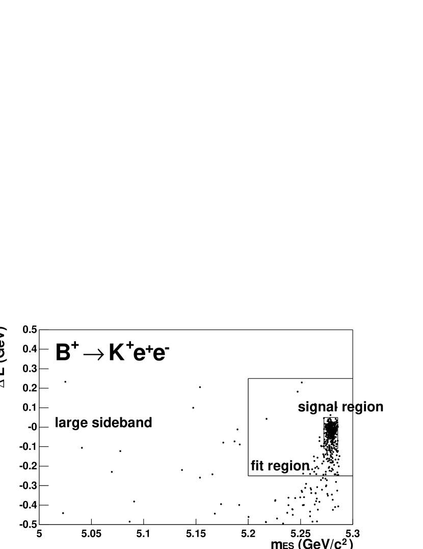
Figure 3 shows three regions that we have defined in the $\Delta E$ vs. $m_{\rm ES}$ plane. The events are taken from a GEANT4 [12] simulation of the process $B^{+}\rightarrow K^{+}e^{+}e^{-}.$ The small box where most of the events lie is the nominal signal region. This region is used to indicate where most of the signal is expected, but signal events are extracted over the full fit region, which is much larger. The fit region is concealed during the process of determining the event selection criteria. The region outside the fit region is called the large sideband. It is not concealed but is instead used to perform data vs. Monte Carlo comparisons in a region that is dominated by combinatorial background. This region, together with samples of $Ke\mu$ and $K^{*}e\mu$ events, provides a way for us to study combinatorial backgrounds without the possibility of biasing the sample of events in the fit region. In the fits, the background normalization is allowed to float, as are other parameters describing the background shape. Thus, while we use Monte Carlo samples to motivate our background parametrizations, the parameter values themselves are not fixed from the Monte Carlo simulation.

       

Figure 3: The distribution of Monte-Carlo-simulated $B^{+}\rightarrow K^{+}e^{+}e^{-}$ events in the $m_{\rm ES}$ vs. $\Delta E$ plane. The nominal signal region, fit region, and large-sideband region are shown. The full fit region in the data is concealed (“blinded”) until the event selection procedure is defined and the data validation steps are performed. The nominal signal region is used only for the optimization of the event selection criteria using Monte Carlo samples; the extraction of the signal yields from the data is based on an analysis of the entire fit region.

5 Event selection

We select events that have at least four charged tracks, the ratio $R_{2}$ of the second and zeroth Fox-Wolfram moments [13] (calculated using charged tracks and unmatched calorimeter clusters) less than 0.5, and two oppositely charged leptons with labratory-frame momenta $p>0.5\ (1.0)\ {\rm GeV}/c$ for $e$ ($\mu$) candidates. The leptons are identified with strict criteria to minimize the misidentification rates for hadrons. The typical probability for a pion to be misidentified as an electron is 0.2% to 0.3%, depending on momentum; the probability for a pion to be misidentified as a muon is 1.3% to 2.7%. Electron-positron pairs consistent with photon conversions in the detector material are vetoed. In the $B\rightarrow Ke^{+}e^{-}$ modes, $e^{+}e^{-}$ pairs at low $q^{2}$ are vetoed independent of the distance of the vertex from the beam axis, but in $B\rightarrow K^{*}e^{+}e^{-}$, where we expect substantial rate at low $q^{2}$, we veto only conversion candidates that occur at a radius of at least 2 cm, where detector materials are present. We require charged kaon candidates to be identified as kaons with strict criteria and the charged pion in $K^{*}\rightarrow K\pi$ not to be identified as a kaon. The use of strict criteria for kaon and lepton identification is necessary to suppress peaking backgrounds. For $B\rightarrow K^{\ast}\ell^{+}\ell^{-}$, we require the mass of the $K^{\ast}$ candidate to be within 75$~{}{\mathrm{\,Me\kern-1.00006ptV\!/}c^{2}}$ of the mean $K^{\ast}(892)$ mass. $K^{0}_{S}$ candidates are reconstructed from two oppositely charged tracks that form a good vertex displaced from the primary vertex by at least 1 mm. The mass of the $\pi^{+}\pi^{-}$ system must be within $\pm 9.3$ MeV/$c^{2}$ of the nominal $K_{S}^{0}$ mass.

The decays $B\rightarrow J/\psi(\rightarrow\ell^{+}\ell^{-})K^{(*)}$ and $B\rightarrow\psi(2S)(\rightarrow\ell^{+}\ell^{-})K^{(*)}$ have identical topologies to signal events. These backgrounds are suppressed by applying a veto in the $\Delta E$ vs. $m_{\ell^{+}\ell^{-}}$ plane (Fig. 4). This veto removes charmonium events not only with reconstructed $m_{\ell^{+}\ell^{-}}$ values near the nominal charmonium masses, but also events that lie further away in $m_{\ell^{+}\ell^{-}}$ due to photon radiation (more pronounced in electron channels) or track mismeasurement. Removing these events—not only from the signal region, but also from the full fit region—simplifies the description of the background shape. Charmonium events can, however, escape this veto if one of the leptons (typically a muon) and the kaon are misidentified as each other. If reassignment of particle types results in a dilepton mass consistent with the $J/\psi$ or $\psi(2S)$ mass, the candidate is vetoed. There is also significant feed-up from $B\rightarrow J/\psi K$ and $B\rightarrow\psi(2S)K$ into $B\rightarrow K^{\ast}\ell^{+}\ell^{-}$, since energy lost due to bremsstrahlung in $B\rightarrow J/\psi K$ can be compensated for by including a random pion. If the $K\ell^{+}\ell^{-}$ system in a $B\rightarrow K^{*}\ell^{+}\ell^{-}$ candidate is kinematically consistent with $B\rightarrow J/\psi(\rightarrow\ell^{+}\ell^{-}\gamma)K$, assuming that the photon (which is not directly observed) was radiated along the direction of either lepton, then the candidate is vetoed. In modes with muons we also apply a veto against backgrounds from $B\rightarrow D\pi$, with $D\rightarrow K^{(*)}\pi$. We reassign the particle hypothesis for the muon candidate with charge consistent to form a $D$ when combined with the $K^{(*)}$ to a pion and veto the candidate if the mass of the muon-$K^{(*)}$ system is consistent with the $D$ mass.

Apart from the charmonium vetoes, we analyze the full range of $q^{2}$. In the $B\rightarrow Ke^{+}e^{-}$, $B\rightarrow K\mu^{+}\mu^{-}$, and $B\rightarrow K^{*}e^{+}e^{-}$ modes, we have good efficiency over most of the $q^{2}$ range, while in the $B\rightarrow K^{*}\mu^{+}\mu^{-}$ mode the efficiency is highest at intermediate and high $q^{2}$ values. This efficiency variation results from the interplay between the lepton identification efficiency and the reconstruction efficiency of the recoil hadron as a function of momentum. The average lepton momentum increases as $q^{2}$ increases; since our minimum momentum requirement is lower for electrons than muons, the region of good lepton efficiency generally extends to lower values of $q^{2}$ for electrons. However, the momentum of the recoil hadron decreases as $q^{2}$ increases, which produces the opposite effect in the $K^{(*)}$ efficiency.

Figure 4: Charmonium veto in the $\Delta E$ vs. $m_{\ell^{+}\ell^{-}}$ plane for (a) $B\rightarrow K^{(*)}e^{+}e^{-}$ and (b) $B\rightarrow K^{(*)}\mu^{+}\mu^{-}$. Hatched regions are vetoed. The dots correspond to a Monte Carlo simulation of $B\rightarrow J/\psi(\rightarrow\ell^{+}\ell^{-})K$ and $B\rightarrow\psi(2S)(\rightarrow\ell^{+}\ell^{-})K$. Most signal events lie in the $\Delta E$ region between the horizontal lines.

Continuum background from non-resonant $e^{+}e^{-}\rightarrow q\overline{q}$ production is suppressed using a Fisher discriminant [14], which is a linear combination of the input variables with optimized coefficients. The variables included are $R_{2}$; $\cos\theta_{B}$, the cosine of the angle between the $B$ candidate and the beam axis in the CM frame; $\cos\theta_{\rm T}$, the cosine of the angle between the thrust axis of the candidate $B$ meson daughter particles and that of the remaining particles in the CM frame; and $m_{K\ell}$, the invariant mass of the $K$-lepton system, where the lepton is selected according to its charge relative to the strangeness of the $K^{(*)}$. The variable $m_{K\ell}$ helps discriminate against background from semileptonic $D$ decays, for which $m_{K^{(*)}\ell}<m_{D}$. The Fisher discriminant is optimized separately for each decay channel.

Combinatorial background from $B\kern 1.79993pt\overline{\kern-1.79993ptB}{}$ events is suppressed using a signal-to-$B\kern 1.79993pt\overline{\kern-1.79993ptB}{}$ likelihood ratio that combines candidate $B$ and dilepton vertex probabilities; the significance of the dilepton separation along the beam direction; $\cos\theta_{B}$; and the missing energy, $E_{\rm miss}$, of the event in the CM frame. The variable $E_{\rm miss}$ provides the strongest discrimination against $B\kern 1.79993pt\overline{\kern-1.79993ptB}{}$ background, since events with semileptonic decays usually have significant unobserved energy due to neutrinos. We construct a likelihood variable because the shape of the $B$ vertex probability distributions are not well suited to a Fisher discriminant. A separate $B$ likelihood variable is constructed for each channel.

For each final state, we select at most one combination of particles per event as a $B$ signal candidate. If multiple candidates occur in the fit region, we select the candidate with the greatest number of drift chamber and SVT hits on the charged tracks. In the $B\rightarrow K\ell^{+}\ell^{-}$ modes less than 1% of the events have multiple candidates and in the $B\rightarrow K^{*}\ell^{+}\ell^{-}$ modes about 10% of the events have more than one candidate. This criterion is designed to be negligibly biased with respect to the kinematic quantities used in our fit.

6 Control sample studies

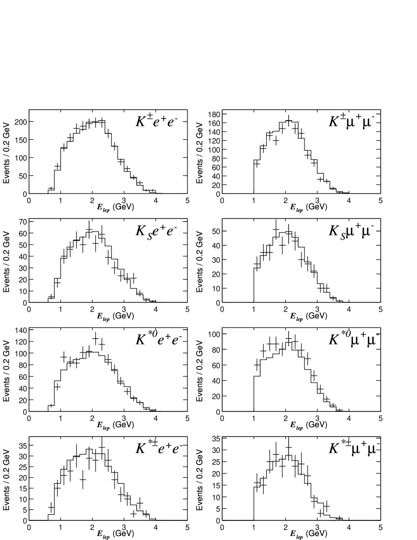
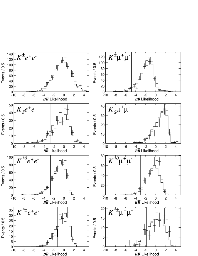
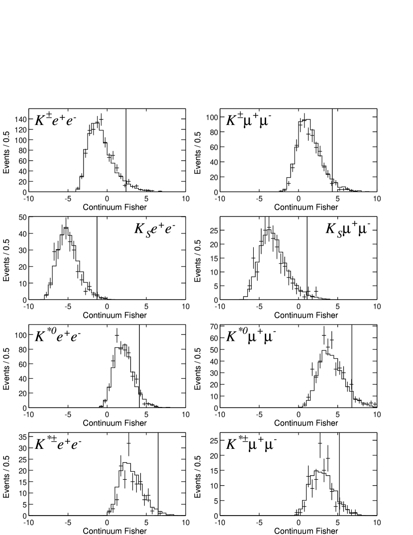
To check the ability of the Monte Carlo to correctly simulate the detector response, we study the charmonium decays $B\rightarrow J/\psi K^{(*)}$ and $B\rightarrow\psi(2S)K^{(*)}$, whose decay distributions and branching fractions are reasonably well known. Figures 5, 6, 7, and 8 compare the distributions of $m_{\ell^{+}\ell^{-}}$, lepton energy in the $\mathchar 28935\relax(4S)$ CM frame, $B$ likelihood variable, and Fisher continuum suppression variable for these signal-like control samples. In each case the distributions are absolutely normalized, so that we are comparing not only the agreement between shapes, but also the agreement between event yields. Table 1 summarizes the event yields in the nominal signal boxes for data and the Monte Carlo prediction in the control samples. We observe good agreement in the yield between data and Monte Carlo simulation in all channels. The agreement in the tails of the dilepton mass distributions indicates that the placement of our charmonium vetoes is based on a reliable simulation. The lepton-energy distributions are well simulated, indicating that the Monte Carlo efficiencies should be well simulated at other values of $q^{2}$. The selections on the $B$ likelihood and Fisher continuum-suppression variables are rather loose, and the agreement between Monte Carlo simulation and data in the control samples indicates that the Monte Carlo efficiencies should be reliable. We discuss these issues quantitatively in the discussion of systematic errors (Sec. 8).

Figure 5: Comparison of the $m_{\ell^{+}\ell^{-}}$ distributions between data and Monte Carlo simulation for the charmonium control samples. The points with error bars show the data, and the solid histograms show the prediction of the charmonium Monte Carlo simulation. All of the analysis selection criteria have been applied except for the charmonium veto, which is reversed. The events are also required to be in the nominal signal region in the $m_{\rm ES}$ vs. $\Delta E$ plane. The large tails in the $e^{+}e^{-}$ modes are due to photon radiation.

Figure 6: Comparison of the lepton-energy distributions between data and Monte Carlo simulation for the charmonium control samples. The points with error bars show the data, and the solid histograms show the prediction of the charmonium Monte Carlo simulation. All of the analysis selection criteria have been applied except for the charmonium veto, which is reversed. The events are also required to be in the nominal signal region in the $m_{\rm ES}$ vs. $\Delta E$ plane.

Figure 7: Comparison of the $B$ likelihood distributions between data and Monte Carlo simulation for the charmonium control samples. The points with error bars show the data, and the solid histograms show the prediction of the charmonium Monte Carlo simulation. All of the analysis selection criteria have been applied except for that on the $B$ likelihood and the charmonium veto, which is reversed. The events are also required to be in the nominal signal region in the $m_{\rm ES}$ vs. $\Delta E$ plane. The vertical lines show the minimum $B$ likelihood values allowed for the corresponding signal modes.

Figure 8: Comparison of the Fisher continuum-suppression variable distributions between data and Monte Carlo simulation for the charmonium control samples. The points with error bars show the data, and the solid histograms show the prediction of the charmonium Monte Carlo simulation. All of the analysis selection criteria have been applied except for that on the Fisher and the charmonium veto, which is reversed. The events are also required to be in the nominal signal region in the $m_{\rm ES}$ vs. $\Delta E$ plane. The vertical lines show the maximum Fisher values allowed for the corresponding signal modes.

Table 1: Comparison of the ${J\mskip-3.0mu/\mskip-2.0mu\psi\mskip 2.0mu}$ control sample event yields in data and Monte Carlo simulations for each of the modes. All selection criteria have been applied, except that the ${J\mskip-3.0mu/\mskip-2.0mu\psi\mskip 2.0mu}$ veto is reversed, and the nominal signal region is selected in $m_{\rm ES}$ and $\Delta E$. The Monte Carlo samples have been scaled to the equivalent number of $\mathchar 28935\relax{(4S)}$ decays in the corresponding data sample. Errors on the ratios of data yields to yields from the Monte Carlo simulation are due to our sample statistics only, and do not incorporate branching fraction uncertainties.

Mode ($J/\psi\rightarrow\ell^{+}\ell^{-})$	MC Yield	Data Yield	Data/MC(%)
$B^{\pm}\rightarrow K^{\pm}e^{+}e^{-}$	911.8	939	${103.0}{\pm 3.8}$
$B^{\pm}\rightarrow K^{\pm}\mu^{+}\mu^{-}$	669.1	623	${93.1}{\pm 4.1}$
$B^{0}\rightarrow K^{0}_{\scriptscriptstyle S}e^{+}e^{-}$	271.6	265	${97.6}{\pm 6.0}$
$B^{0}\rightarrow K^{0}_{\scriptscriptstyle S}\mu^{+}\mu^{-}$	195.0	191	${98.0}{\pm 7.1}$
$B^{0}\rightarrow K^{*0}e^{+}e^{-}$	494.5	523	${105.8}{\pm 4.9}$
$B^{0}\rightarrow K^{*0}\mu^{+}\mu^{-}$	353.7	412	${116.5}{\pm 6.2}$
$B^{\pm}\rightarrow K^{*\pm}e^{+}e^{-}$	158.6	144	${90.8}{\pm 7.7}$
$B^{\pm}\rightarrow K^{*\pm}\mu^{+}\mu^{-}$	106.4	111	${104.4}{\pm 10.2}$
Combined by hadron final state
$B^{\pm}\rightarrow K^{\pm}\ell^{+}\ell^{-}$	1580.9	1562	${98.8}{\pm 2.8}$
$B^{0}\rightarrow K^{0}_{\scriptscriptstyle S}\ell^{+}\ell^{-}$	466.5	456	${97.7}{\pm 4.6}$
$B^{0}\rightarrow K^{*0}\ell^{+}\ell^{-}$	848.2	935	${110.2}{\pm 3.9}$
$B^{\pm}\rightarrow K^{*\pm}\ell^{+}\ell^{-}$	264.9	255	${96.3}{\pm 6.2}$
Combined by lepton final state
$e^{+}e^{-}$ modes	1836.4	1871	${101.9}{\pm 2.6}$
$\mu^{+}\mu^{-}$ modes	1324.1	1337	${101.0}{\pm 3.0}$
all modes	3160.5	3208	${101.5}{\pm 1.9}$

The large sidebands provide a useful tool for monitoring our simulation of the combinatorial backgrounds. In contrast to the charmonium control samples, the events here are produced by a wide variety of processes, including both $B\overline{B}$ and continuum. We compare the distributions observed in data with the sum of $B\overline{B}$ Monte Carlo simulations and continuum samples obtained from off-resonance data. Although the off-resonance sample is statistically limited, it gives a correct picture of the complicated mix of $q\overline{q}$, $\tau^{+}\tau^{-}$, and two-photon events. Figure 9 shows the distribution of the $B$ likelihood variable in the large sideband. Both the shapes and the normalizations are reasonably well predicted. There are large fluctuations in the off-resonance data sample, which is scaled by a factor of about 8 to correspond to the integrated luminosity of the on-resonance data sample.

Figure 9: Large sideband comparison of the $B$ likelihood variable distributions between data and $B\overline{B}$ Monte Carlo simulation plus scaled off-resonance data. The points with error bars show the on-resonance data, the shaded histograms show the scaled off-resonance data, and the open histograms show the sum of the scaled off-resonance data and the $B\overline{B}$ Monte Carlo sample. All of the analysis selection criteria have been applied except for that on the $B\overline{B}$ likelihood. The position of this cut is indicated by vertical lines; selected events are required to have $B$ likelihood above this value.

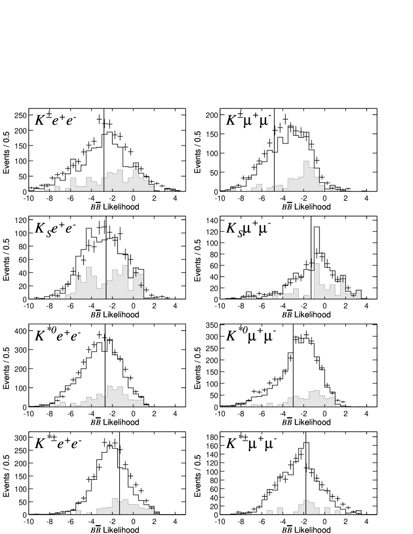
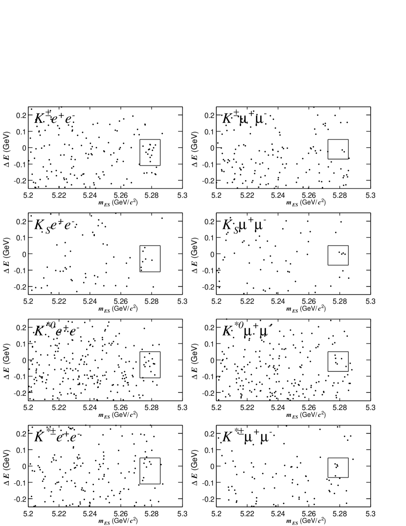
For each data taking period, we check the control samples in the manner described above. We then “unblind” the data in the fit region. The distributions of the data for each mode are shown in Fig. 10. In several of the modes, a small number of events is present in the nominal signal region. For the events in the nominal signal region we show the dilepton mass distribution in Fig. 11. The prediction based on our simulation of the signal is also shown.

Figure 10: Distribution of the data in the $\Delta E$ vs. $m_{\rm ES}$ plane (fit region) for each channel. The rectangles show the nominal signal boxes, but the signals are extracted from a two-dimensional fit.

Figure 11: The dilepton mass distribution for data (points with error bars) and signal Monte Carlo (histogram) for events in the nominal signal region. The data include some amount of background, so the distributions are not expected to agree perfectly. However, the data do not cluster around the charmonium veto regions; such clustering would be a possible indication of charmonium background events escaping the veto.

7 Fits and yields

We extract the signal and background yields in each channel using a two-dimensional extended unbinned maximum likelihood fit in the region defined by $m_{\rm ES}$ $>$ 5.2 GeV/$c^{2}$ and $|\Delta E|$ $<$ 0.25 GeV (“fit region”). The two-dimensional signal shapes, including the effects of radiation on the $\Delta E$ distribution and the correlation between $m_{\rm ES}$ and $\Delta E$, are obtained by parameterizing a GEANT4 Monte Carlo simulation of the signal using the product of two Crystal Ball shapes [15], one for $m_{\rm ES}$ and one for $\Delta E$. The Crystal Ball shape smoothly matches a Gaussian core with a tail that is used to describe radiative effects. For $m_{\rm ES}$ we use a single Gaussian core, while in $\Delta E$ we describe the core using the sum of two Gaussians with separate mean and width. The parameters in the Crystal Ball shape for $m_{\rm ES}$ are allowed to have a quadratic dependence on $\Delta E$, which adequately takes into account the correlation between $m_{\rm ES}$ and $\Delta E$. Small shifts in the mean values of $m_{\rm ES}$ and $\Delta E$ are applied to the signal shapes based on studies of these quantities in the charmonium control samples.

The combinatorial background is described by the function

$$f(\mbox{$\Delta E$},\mbox{$m_{\rm ES}$})=Ne^{s\Delta E}\mbox{$m_{\rm ES}$}\sqrt{1-{\mbox{$m_{\rm ES}$}^{2}\over E_{\rm b}^{2}}}e^{-\xi\left(1-{m_{\rm ES}^{2}\over E_{\rm b}^{2}}\right)},$$

where $N$ is a normalization factor, and $s$ and $\xi$ are free parameters determined in the fit to the data. The part of this function that describes the $m_{\rm ES}$ distribution is a standard form known as the ARGUS function [16].

For systematic studies we also use a more general form for the background shape, where the ARGUS slope parameter, $\xi$, is allowed to be a function of $\Delta E$:

$$\xi=\xi(\Delta E)=\xi_{0}+\xi_{1}\Delta E+{1\over 2}\xi_{2}(\Delta E)^{2}.$$

In each channel we also include a term to describe the estimated amount of background that peaks under the signal. Peaking backgrounds can arise from $B\rightarrow K^{*}\gamma$ followed by a photon conversion in the detector material or from decays such as $B\rightarrow K\pi\pi$ in which the pions are misidentified as leptons. Our estimates for these backgrounds are obtained from specific studies of individual processes and make use of hadron misidentification rates measured in data. The total estimated peaking background for each mode is listed in Table 2.

Table 2: Summary of peaking backgrounds used in the fits.

Mode	Peaking background (events)
$B^{\pm}\rightarrow K^{\pm}e^{+}e^{-}$	$0.0^{+1.0}_{-0.0}$
$B^{\pm}\rightarrow K^{\pm}\mu^{+}\mu^{-}$	$0.7\pm 0.7$
$B^{0}\rightarrow K^{0}_{\scriptscriptstyle S}e^{+}e^{-}$	$0.0^{+0.1}_{-0.0}$
$B^{0}\rightarrow K^{0}_{\scriptscriptstyle S}\mu^{+}\mu^{-}$	$0.5\pm 0.5$
$B^{0}\rightarrow K^{*0}e^{+}e^{-}$	$0.2^{+0.5}_{-0.2}$
$B^{0}\rightarrow K^{*0}\mu^{+}\mu^{-}$	$1.2\pm 1.2$
$B^{\pm}\rightarrow K^{*\pm}e^{+}e^{-}$	$0.1^{+0.4}_{-0.1}$
$B^{\pm}\rightarrow K^{*\pm}\mu^{+}\mu^{-}$	$1.0\pm 1.0$

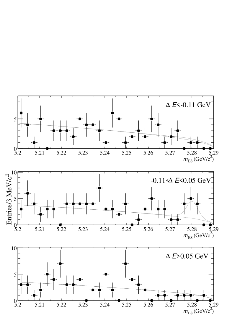
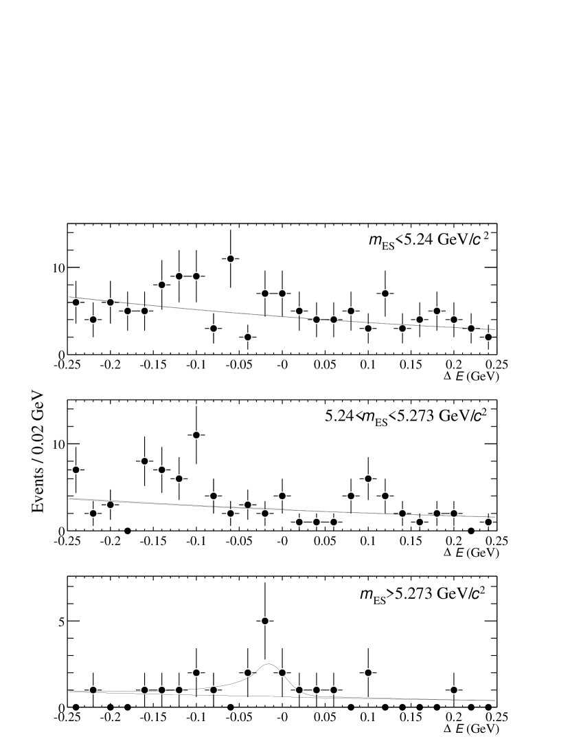
As an example, we present the fits for the $B\rightarrow K^{*0}e^{+}e^{-}$ mode. Figure 12 shows the $m_{\rm ES}$ distributions in three slices of $\Delta E$ that span the fit region: $\Delta E<0.11$ GeV, $-0.11\leq\Delta E<0.05$ GeV, and $\Delta E\geq 0.05$ GeV. We observe a peak in $m_{\rm ES}$ around the $B$ mass for the range $-0.11\leq\Delta E<0.05$ GeV, but not in the upper or lower $\Delta E$ sidebands. Figure 13 shows the distributions of the data in $\Delta E$ for three slices of $m_{\rm ES}$: $m_{\rm ES}<5.24$ GeV$/c^{2}$, $5.24\leq m_{\rm ES}<5.273$ GeV$/c^{2}$, $m_{\rm ES}\geq 5.273$ GeV$/c^{2}$.

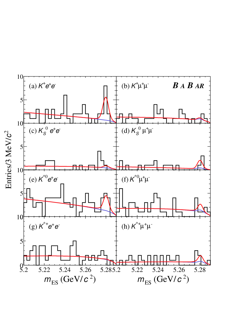
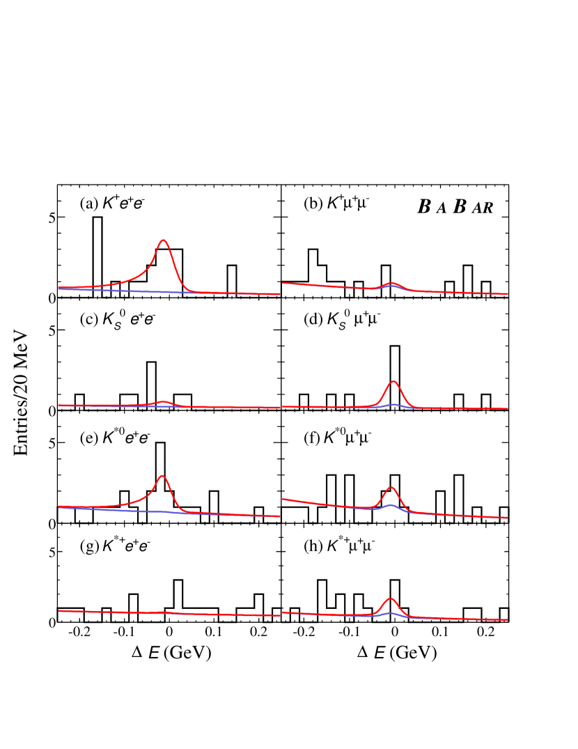
Figure 14 shows the projections of the fits for each channel onto $m_{\rm ES}$ for $\Delta E$ in the nominal signal regions. Figure 15 shows the projections of the fits for each channel onto $\Delta E$ for $m_{\rm ES}$ in the nominal signal regions. We observe small excesses of events over the backgrounds in several channels. Table 3 summarizes the results for each channel.

Table 3: Results from individual fits to $B$ $\rightarrow$ $K^{(*)}$$\ell^{+}\ell^{-}$ modes. The columns are, from left to right: (1) the fitted signal yield; (2) the contribution of the background to the error on the signal yield, expressed as an effective background yield; (3) the signal efficiency, $\epsilon$ (not including the branching fractions for $K^{*}$, $K^{0}$, and $K^{0}_{\scriptscriptstyle S}$ decays); (4) the multiplicative systematic error on the selection efficiency, $(\Delta{\cal B}/{\cal B})_{\epsilon}$; (5) the additive systematic error from the fit, $(\Delta{\cal B})_{\rm fit}$; and (6) the branching fraction central value ($\cal B$).

Mode	Signal	Effective	$\epsilon$	($\Delta{\cal B}/{\cal B})_{\epsilon}$	$(\Delta{\cal B})_{\rm fit}$	$\qquad{\cal B}$
	Yield	Bkgnd.	(%)	(%)	$(/10^{-6})$	$(/10^{-6})$
$B^{+}\rightarrow K^{+}e^{+}e^{-}$	$14.4^{+5.0}_{-4.2}$	2.2	17.5	$\pm 6.8$	${}^{+0.14}_{-0.21}$	$0.98^{+0.34+0.16}_{-0.28-0.22}$
$B^{+}\rightarrow K^{+}\mu^{+}\mu^{-}$	$0.5^{+2.3}_{-1.3}$	2.2	9.2	$\pm 6.6$	${}^{+0.09}_{-0.08}$	$0.06^{+0.30+0.09}_{-0.17-0.08}$
$B^{0}\rightarrow K^{0}e^{+}e^{-}$	$1.3^{+2.6}_{-1.7}$	1.5	18.6	$\pm 7.9$	$\pm 0.14$	$0.24^{+0.49+0.14}_{-0.32-0.15}$
$B^{0}\rightarrow K^{0}\mu^{+}\mu^{-}$	$3.6^{+2.9}_{-2.1}$	0.9	9.4	$\pm 7.7$	$\pm 0.24$	$1.33^{+1.07}_{-0.78}\pm 0.26$
$B^{0}\rightarrow K^{*0}e^{+}e^{-}$	$10.6^{+5.2}_{-4.3}$	5.5	10.6	$\pm 7.6$	${}^{+0.46}_{-0.47}$	$1.78^{+0.87+0.48}_{-0.72-0.49}$
$B^{0}\rightarrow K^{*0}\mu^{+}\mu^{-}$	$3.4^{+3.9}_{-2.8}$	4.6	6.1	$\pm 9.3$	$\pm 0.38$	$0.99^{+1.14}_{-0.82}\pm 0.39$
$B^{+}\rightarrow K^{*+}e^{+}e^{-}$	$0.3^{+3.7}_{-2.3}$	6.3	10.3	$\pm 9.5$	${}^{+0.69}_{-0.72}$	$0.15^{+1.87+0.69}_{-1.16-0.72}$
$B^{+}\rightarrow K^{*+}\mu^{+}\mu^{-}$	$3.6^{+3.9}_{-2.5}$	3.4	5.2	$\pm 11.1$	$\pm 1.80$	$3.61^{+3.91}_{-2.51}\pm 1.84$

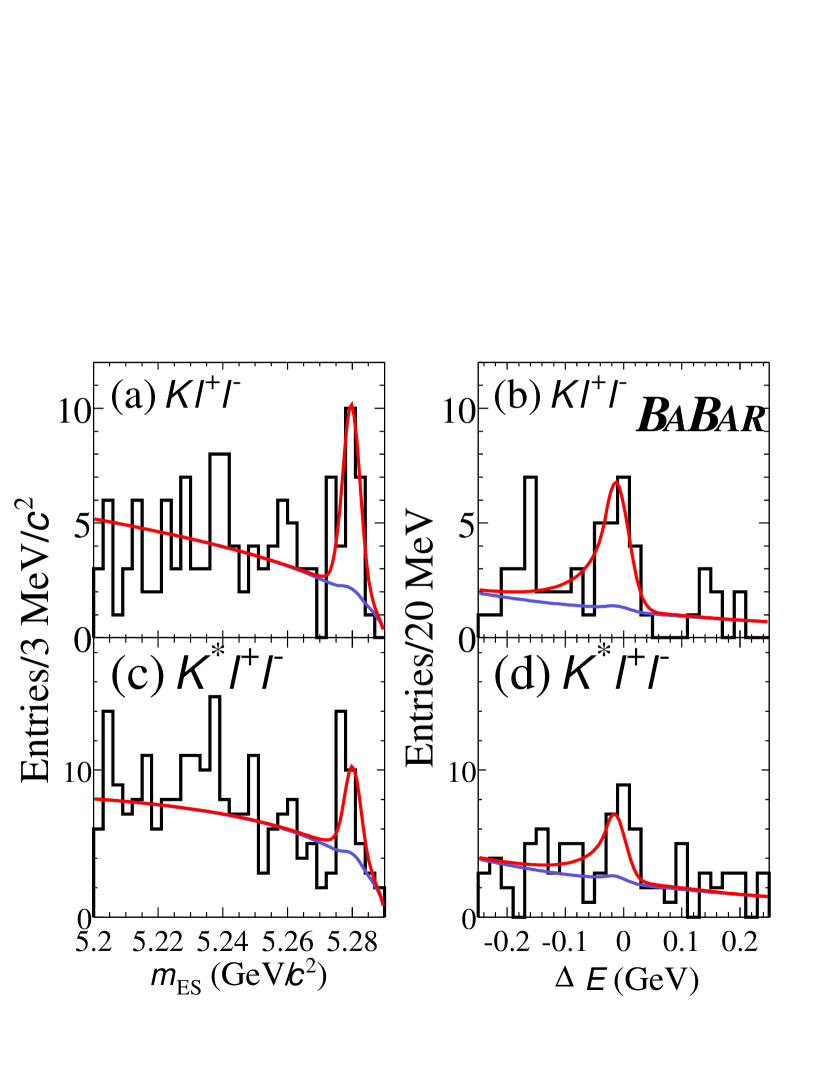
We also perform combined fits in which the branching fractions in the four $B\rightarrow K\ell^{+}\ell^{-}$ channels are constrained to each other, as are the branching fractions for the four $B\rightarrow K^{*}\ell^{+}\ell^{-}$ channels (Fig. 16). Due to the larger pole at low values of $m_{\ell^{+}\ell^{-}}$ in $B\rightarrow K^{*}e^{+}e^{-}$ than in $B\rightarrow K^{*}\mu^{+}\mu^{-}$, the expected rates for these channels differ and are constrained to the ratio of branching fractions ${\cal B}(B\rightarrow K^{*}e^{+}e^{-})/{\cal B}(B\rightarrow K^{*}\mu^{+}\mu^{-})=1.2$ from the model of Ali et al. [1]. The extracted yield corresponds to the electron mode. The branching fractions from the combined fits, with statistical errors only, are

$${\cal B}(B\rightarrow K\ell^{+}\ell^{-}) = (0.78^{+0.24}_{-0.20}(\rm stat.))\times 10^{-6},$$

$${\cal B}(B\rightarrow K^{*}\ell^{+}\ell^{-}) = (1.68^{+0.68}_{-0.58}(\rm stat.))\times 10^{-6}.$$

Figure 12: Fit to the data for the mode $B^{0}\rightarrow K^{*0}(\rightarrow K^{+}\pi^{-})e^{+}e^{-}$. The three histograms show the $m_{\rm ES}$ distributions in three slices of $\Delta E$: $\Delta E<-0.11$ GeV, $-0.11\leq\Delta E<0.05$ GeV, and $\Delta E\geq 0.05$ GeV.

Figure 13: Fit to the data for the mode $B^{0}\rightarrow K^{*0}(\rightarrow K^{+}\pi^{-})e^{+}e^{-}$. The three histograms show the $\Delta E$ distributions in three slices of $m_{\rm ES}$: $m_{\rm ES}<5.24$ GeV$/c^{2}$, $5.24\leq m_{\rm ES}<5.273$ GeV$/c^{2}$, $m_{\rm ES}\geq 5.273$ GeV$/c^{2}$. The peak in $\Delta E$ near zero in the lower histogram is correlated with the peak in $m_{\rm ES}$ around the $B$ mass.

Figure 14: Projections of the individual fits onto the $m_{\rm ES}$ distributions for the slice $-0.11\leq\Delta E<0.05$ GeV (electron modes) or $-0.07\leq\Delta E<0.05$ GeV (muon modes).

Figure 15: Projections of the individual fits onto the $\Delta E$ distributions for $m_{\rm ES}$ in the nominal signal regions.

Figure 16: Summed distributions for the four $B\rightarrow K\ell^{+}\ell^{-}$ and the four $B\rightarrow K^{*}\ell^{+}\ell^{-}$ channels, showing the projections of the combined fit. In this combined fit, the yields in the $B\rightarrow K\ell^{+}\ell^{-}$ channels are constrained to each other, as are the yields in the $B\rightarrow K^{*}\ell^{+}\ell^{-}$ channels (see text).

8 Systematic uncertainties

Systematic errors arise from uncertainties on the efficiency and on the number of $B\overline{B}$ pairs in the data sample (both of which are multiplicative errors) and on the yields extracted from the fits (additive systematic errors).

Table 4 summarizes the multiplicative systematic uncertainties. The systematic uncertainty from the continuum Fisher and $B\kern 1.79993pt\overline{\kern-1.79993ptB}{}$ likelihood selection criteria are determined from the differences of efficiency for these criteria in data and Monte Carlo simulations for charmonium control samples (see Figures 7 and 8). The uncertainties on the efficiencies due to model-dependence of form factors are taken to be the full range of variation obtained from different theoretical models [1]. The total multiplicative systematic uncertainty is the sum in quadrature of the individual sources, with the exception of the tracking efficiency uncertainties for leptons and hadrons, which are taken to be 100% correlated. The total uncertainty ranges from 7–11%; the largest individual source is the theoretical model dependence of the signal efficiency, which ranges from 4–7%. The combined multiplicative systematic errors are also listed in Table 3.

Table 4: Multiplicative systematic uncertainties.

Systematic	$K^{+}e^{+}e^{-}$	$K^{+}\mu^{+}\mu^{-}$	$K_{S}^{0}e^{+}e^{-}$	$K_{S}^{0}\mu^{+}\mu^{-}$	$K^{*0}e^{+}e^{-}$	$K^{*0}\mu^{+}\mu^{-}$	$K^{*+}e^{+}e^{-}$	$K^{*+}\mu^{+}\mu^{-}$
Trk eff. ($e,\mu$)	$\pm 1.6$	$\pm 1.6$	$\pm 1.6$	$\pm 1.6$	$\pm 1.6$	$\pm 1.6$	$\pm 1.6$	$\pm 1.6$
Electron ID	$\pm 2.7$	-	$\pm 2.7$	-	$\pm 2.7$	-	$\pm 2.7$	-
Muon ID	-	$\pm 2.0$	-	$\pm 2.0$	-	$\pm 2.0$	-	$\pm 2.0$
$K,\pi$ ID	$\pm 2.0$	$\pm 2.0$	-	-	$\pm 4.0$	$\pm 4.0$	$\pm 2.0$	$\pm 2.0$
Trk eff. ($K,\pi$)	$\pm 1.3$	$\pm 1.3$	$\pm 2.6$	$\pm 2.6$	$\pm 2.6$	$\pm 2.6$	$\pm 3.9$	$\pm 3.9$
$K_{S}^{0}$ eff.	-	-	$\pm 3.2$	$\pm 3.2$	-	-	$\pm 3.2$	$\pm 3.2$
$B\overline{B}$ Counting	$\pm 1.1$	$\pm 1.1$	$\pm 1.1$	$\pm 1.1$	$\pm 1.1$	$\pm 1.1$	$\pm 1.1$	$\pm 1.1$
Fisher	$\pm 1.5$	$\pm 1.5$	$\pm 1.5$	$\pm 1.5$	$\pm 1.5$	$\pm 1.5$	$\pm 1.5$	$\pm 1.5$
$B\overline{B}$ likelihood	$\pm 2.5$	$\pm 2.5$	$\pm 2.5$	$\pm 2.5$	$\pm 2.5$	$\pm 2.5$	$\pm 2.5$	$\pm 2.5$
Model dep.	$\pm 4.0$	$\pm 4.0$	$\pm 4.0$	$\pm 4.0$	$\pm 4.0$	$\pm 7.0$	$\pm 4.0$	$\pm 7.0$
MC statistics	$\pm 1.1$	$\pm 1.1$	$\pm 1.1$	$\pm 1.1$	$\pm 1.9$	$\pm 1.6$	$\pm 1.0$	$\pm 1.9$
Total	$\pm 6.8$	$\pm 6.6$	$\pm 7.9$	$\pm 7.7$	$\pm 7.6$	$\pm 9.3$	$\pm 9.5$	$\pm 11.1$

The additive systematic errors are uncertainties in the signal yield from the fit. These arise from three sources: (1) uncertainties in the signal shapes, (2) uncertainties in the background shapes, and (3) uncertainties in the amount of peaking backgrounds. Note that because the background shapes and yields float in the fit, much of the uncertainty associated with the background is automatically incorporated in the statistical uncertainty of the signal. A systematic uncertainty in the background shape is evaluated by (1) fixing the $m_{\rm ES}$ slopes to the values obtained from Monte Carlo simulations rather than allowing the slopes to float in the fit and (2) performing alternative fits in which the $m_{\rm ES}$ slope is allowed to have a quadratic dependence on $\Delta E$, as described above.

The $B^{+}\rightarrow K^{+}e^{+}e^{-}$ channel has one additional systematic uncertainty included. In this channel we observe two events with the following property: if the electrons are each assigned pion masses, then the system is consistent with coming from the decay $B^{+}\rightarrow D^{0}\pi^{+}$; $D^{0}\rightarrow K^{-}\pi^{+}$. The predicted number of such events, based on measured probabilities for pions to be misidentified as electrons, is only about 0.08 event. In spite of this small estimated probability we take into account the possibility that these events might in fact be background by including an asymmetric systematic error corresponding to the subtraction of two events. This issue does not arise in the muon channels, where we have an explicit veto on this background to handle the much higher probability for a pion to be misidentified as a muon.

Table 5 summarizes the additive systematic errors, expressed directly in terms of errors on signal event yields. Table 3 gives the total additive systematic errors propagated to the branching fractions. For the combined fits for $B\rightarrow K\ell^{+}\ell^{-}$ and $B\rightarrow K^{*}\ell^{+}\ell^{-}$ the systematic errors are calculated by weighting the systematic errors from the individual modes based on the expected signal from the efficiency and branching fractions.

Table 5: The sources of additive systematic uncertainty, expressed directly as uncertainties in the signal yield.

Systematic	$K^{+}e^{+}e^{-}$	$K^{+}\mu^{+}\mu^{-}$	$K_{S}^{0}e^{+}e^{-}$	$K_{S}^{0}\mu^{+}\mu^{-}$	$K^{*0}e^{+}e^{-}$	$K^{*0}\mu^{+}\mu^{-}$	$K^{*+}e^{+}e^{-}$	$K^{*+}\mu^{+}\mu^{-}$
Signal shape	$\pm 0.3$	$\pm 0.0$	$\pm 0.3$	$\pm 0.1$	$\pm 0.4$	$\pm 0.2$	$\pm 0.4$	$\pm 0.3$
Comb bkg. shape	$\pm 1.8$	$\pm 0.1$	$\pm 0.7$	$\pm 0.3$	$\pm 2.6$	$\pm 0.3$	$\pm 1.3$	$\pm 1.4$
Peaking bkg.	${}^{+0.0}_{-2.2}$	$\pm 0.7$	${}^{+0.0}_{-0.1}$	$\pm 0.5$	${}^{+0.2}_{-0.5}$	$\pm 1.2$	${}^{+0.1}_{-0.4}$	$\pm 1.0$

9 Discussion

This analysis has yielded preliminary evidence for the decay $B\rightarrow K\ell^{+}\ell^{-}$. The signal events are primarily in the $B^{+}\rightarrow K^{+}e^{+}e^{-}$ channel, although there is also an excess in $B^{0}\rightarrow K_{S}^{0}\mu^{+}\mu^{-}$. The higher event yield in electron over muon channels is not unexpected, due to the substantially higher detection efficiency for electrons than muons in the BABAR detector. The significance of this signal, based purely on the statistical errors, is $5.6\sigma$; when systematic uncertainties are applied, the estimated significance becomes $4.4\sigma$. We conclude that a signal for $B\rightarrow K\ell^{+}\ell^{-}$ has been observed. The measured branching fraction is consistent with most predictions, although the central value of ${\mathcal{B}}(B\rightarrow K\ell^{+}\ell^{-})=(0.78^{+0.24+0.11}_{-0.20-0.18})\times 10^{-6}$ is higher than the Ali et al. prediction of ${\cal B}(B\rightarrow K\ell^{+}\ell^{-})=(0.35\pm 0.12)\times 10^{-6}$. The result is also consistent with Belle’s measurement, ${\cal B}(B\rightarrow K\ell^{+}\ell^{-})=(0.75^{+0.25}_{-0.21}\pm 0.09)\times 10^{-6}$. The result from this 77.8 fb^-1 sample is also higher than the 90% C.L. upper limit obtained from our original analysis of 20.7 fb^-1; the larger data set includes the smaller data set. We have made a conservative evaluation of the consistency in our results as follows: We evaluate the $B\rightarrow K\ell^{+}\ell^{-}$ branching fraction using only the data acquired after that used in the published result. Assuming a true value equal to the result obtained in this newer dataset, we find a 3% probability ($1.9\sigma$) that we would have observed a yield smaller than our published result from the earlier dataset.

We also observe an excess of events in $B\rightarrow K^{*}\ell^{+}\ell^{-}$, with a significance including systematic uncertainty of $2.8\sigma$. We obtain a central value of ${\mathcal{B}}(B\rightarrow K^{*}\ell^{+}\ell^{-})=(1.68^{+0.68}_{-0.58}\pm 0.28)\times 10^{-6}$ and a 90% C.L. upper limit ${\mathcal{B}}(B\rightarrow K^{*}\ell^{+}\ell^{-})<3.0\times 10^{-6}$. The central value is within the range expected in the Standard Model, although the uncertainties are still large.

10 Conclusions

We present preliminary results of our search for $B\rightarrow K^{(*)}\ell^{+}\ell^{-}$ using a sample of $84.4\times 10^{6}$ $B\overline{B}$ pairs produced at the $\mathchar 28935\relax(4S)$. We observe a signal for $B\rightarrow K\ell^{+}\ell^{-}$ with

$${\cal B}(B\rightarrow K\ell^{+}\ell^{-}) = (0.78^{+0.24+0.11}_{-0.20-0.18})\times 10^{-6}.$$

The significance is estimated to be $4.4\sigma$. For $B\rightarrow K^{*}\ell^{+}\ell^{-}$ we obtain

$${\cal B}(B\rightarrow K^{*}\ell^{+}\ell^{-}) = (1.68^{+0.68}_{-0.58}\pm 0.28)\times 10^{-6},$$

using the constraint ${\cal B}(B\rightarrow K^{*}e^{+}e^{-})/{\cal B}(B\rightarrow K^{*}\mu^{+}\mu^{-})=1.2$. For the combined $B\rightarrow K^{*}\ell^{+}\ell^{-}$ result we quote the branching fraction corresponding to the electron channel. The significance of the $B\rightarrow K^{*}\ell^{+}\ell^{-}$signal is estimated to be $2.8\sigma$ and we quote a 90% C.L. limit for this mode of

$${\cal B}(B\rightarrow K^{*}\ell^{+}\ell^{-}) < 3.0\times 10^{-6}.$$

11 Acknowledgments

We are grateful for the extraordinary contributions of our PEP-II colleagues in achieving the excellent luminosity and machine conditions that have made this work possible. The success of this project also relies critically on the expertise and dedication of the computing organizations that support BABAR. The collaborating institutions wish to thank SLAC for its support and the kind hospitality extended to them. This work is supported by the US Department of Energy and National Science Foundation, the Natural Sciences and Engineering Research Council (Canada), Institute of High Energy Physics (China), the Commissariat à l’Energie Atomique and Institut National de Physique Nucléaire et de Physique des Particules (France), the Bundesministerium für Bildung und Forschung and Deutsche Forschungsgemeinschaft (Germany), the Istituto Nazionale di Fisica Nucleare (Italy), the Research Council of Norway, the Ministry of Science and Technology of the Russian Federation, and the Particle Physics and Astronomy Research Council (United Kingdom). Individuals have received support from the A. P. Sloan Foundation, the Research Corporation, and the Alexander von Humboldt Foundation.

References

- [1] A. Ali et al., Phys. Rev. D 61, 074024 (2000); P. Colangelo et al., Phys. Rev. D 53, 3672 (1996); D. Melikhov, N. Nikitin, and S. Simula, Phys. Rev. D 57, 6814 (1998).
- [2] T.M. Aliev et al., Phys. Lett. B 400, 194 (1997); T.M. Aliev, M. Savci, and A. Özpineci, Phys. Rev. D 56, 4260 (1997); M. Beneke, Th. Feldmann, and D. Seidel, Nucl. Phys. B 612, 25 (2001); G. Burdman, Phys. Rev. D 52, 6400 (1995); N.G. Deshpande and J. Trampetic, Phys. Rev. Lett. 60, 2583 (1988); C. Greub, A. Ioannissian, and D. Wyler, Phys. Lett. B 346, 149 (1995); J.L. Hewett and J.D. Wells, Phys. Rev. D 55, 5549 (1997); C.Q. Geng and C.P. Kao, Phys. Rev. D 54, 5636 (1996); and references therein.
- [3] A. Ali, E. Lunghi, C. Greub, and G. Hiller, hep-ph/0112300, to appear in Phys. Rev. D.
- [4] BABAR Collaboration, B. Aubert et al., Phys. Rev. Lett. 88, 241801 (2002).
- [5] Belle Collaboration, K. Abe et al., Phys. Rev. Lett. 88, 021801 (2002).
- [6] CDF Collaboration, T. Affolder et al., Phys. Rev. Lett. 83, 3378 (1999).
- [7] CLEO Collaboration, S. Anderson et al., Phys. Rev. Lett. 87, 181803 (2001).
- [8] CLEO Collaboration, R. Ammar et al., Phys. Rev. Lett. 71, 674 (1993).
- [9] CLEO Collaboration, M.S. Alam et al., Phys. Rev. Lett. 74, 2885 (1995).
- [10] Particle Data Group, K. Hagiwara et al., Phys. Rev. D 66, 010001 (2002).
- [11] BABAR Collaboration, B. Aubert et al., Nucl. Instrum. Methods A 479, 1 (2001).
- [12] GEANT4, Geant4 Collaboration, CERN-IT-2002-003, submitted to Nucl. Instrum. Methods.
- [13] G.C. Fox and S. Wolfram, Phys. Rev. Lett. 41, 1581 (1978).
- [14] R.A. Fisher, Ann. Eugenics 7, 179 (1936).
- [15] T. Skwarnicki, “A Study of the Radiative Cascade Transitions between the Upsilon-Prime and Upsilon Resonances,” DESY F31-86-02 (thesis, unpublished)(1986).
- [16] ARGUS Collaboration, H. Albrecht et al., Phys. Lett. B 241, 278 (1990).