A search for the exclusive radiative decays $B\rightarrow\rho(770)\gamma$ and $B^{0}\rightarrow\omega(782)\gamma$ is performed on a sample of 84 million $B\kern 1.79993pt\overline{\kern-1.79993ptB}{}$ events collected by the BABAR detector at the $PEP-II$ asymmetric $e^{+}e^{-}$ collider. No significant signal is seen in any of the channels. We set preliminary upper limits of ${\cal B}[B^{0}\rightarrow\rho^{0}\gamma]<1.4\times 10^{-6}$, ${\cal B}[B^{+}\rightarrow\rho^{+}\gamma]<2.3\times 10^{-6}$ and ${\cal B}[B^{0}\rightarrow\omega\gamma]<1.2\times 10^{-6}$ at $90\%$ Confidence Level. Combining these into a single limit on the generic process $B\rightarrow\rho\gamma$, we find the preliminary limit ${\cal B}[B\rightarrow\rho\gamma]<1.9\times 10^{-6}$ corresponding, to a limit of $\cal B$[$B\rightarrow\rho\gamma$]/$\cal B$[$B\rightarrow K^{*}\gamma$] $<$ $0$.047 at $90\%$ Confidence Level.

1 Introduction

The effective flavor-changing neutral current processes $B\rightarrow\rho\gamma$ and $B^{0}\rightarrow\omega\gamma$ probe physics at high mass scales both within the Standard Model and within the context of possible new physics scenarios through the underlying $b\rightarrow d\gamma$ “penguin” transition [1]. The decays are analogous to the $B\rightarrow K^{*}\gamma$ process mediated by the $b\rightarrow s\gamma$ transition. The expected rate of $b\rightarrow d\gamma$ transitions is suppressed by the ratio of CKM matrix elements $|V_{td}/V_{ts}|^{2}$ relative to $b\rightarrow s\gamma$ transitions. There has been considerable interest recently in these exclusive channels, resulting in several calculations of the branching fractions expected in the Standard Model, which indicate a range ${\cal B}[B^{+}\rightarrow\rho^{+}\gamma]=(0.9-1.5)\times 10^{-6}$ [2]. Though the theoretical uncertainties for the branching fractions remain large, the possibility of extracting the ratio of CKM elements $|V_{td}/V_{ts}|^{2}$ through the ratio ${\cal B}[B\rightarrow(\rho/\omega)\gamma]/{\cal B}[B\rightarrow K^{*}\gamma]$ with less uncertainty has been explored [3][4]. The observation of $B\rightarrow\rho\gamma$ and $B^{0}\rightarrow\omega\gamma$ would constitute the first evidence of the $b\rightarrow d\gamma$ radiative transition and is of considerable interest as the first step towards extracting $|V_{td}/V_{ts}|$ from measurements of these channels. Previous searches have found no evidence for these decays [5].

2 The BABAR Detector and Dataset

The decay $B\rightarrow\rho\gamma$ is reconstructed in the modes $B^{0}\rightarrow\rho^{0}\gamma$ with $\rho^{0}\rightarrow\pi^{+}\pi^{-}$ and $B^{+}\rightarrow\rho^{+}\gamma$ with $\rho^{+}\rightarrow\pi^{+}\pi^{0}$ (charge-conjugate modes are implied throughout), while $B^{0}\rightarrow\omega\gamma$ is reconstructed with $\omega\rightarrow\pi^{+}\pi^{-}\pi^{0}$. The analysis uses a sample of 84 million $B\kern 1.79993pt\overline{\kern-1.79993ptB}{}$ events in $78\mbox{\,fb}^{-1}$ of data collected by the BABAR detector [6] at the $PEP-II$ collider [7] on the $\mathchar 28935\relax{(4S)}$ resonance (“on-resonance”), and $9.6\mbox{\,fb}^{-1}$ of data taken $40{\mathrm{\,Me\kern-1.00006ptV\!/}c^{2}}$ below the $\mathchar 28935\relax{(4S)}$ resonance (“off-resonance”). The reconstruction uses quantities both in the laboratory and $\mathchar 28935\relax{(4S)}$ center-of-mass (CMS) frames, where the latter are denoted by an asterisk. The detector response to the signal and background processes are studied with a detailed Monte Carlo simulation based on Geant4 [8] and cross-checked with control samples in the data. The off-resonance data provide a control sample of the primary backgrounds from the continuum production of $u$, $d$, $s$, and $c$ quark-antiquark pairs, while exclusively reconstructed $B\rightarrow D\pi$ decays provide a sample to cross-check the simulation of $B\kern 1.79993pt\overline{\kern-1.79993ptB}{}$ events.

3 Analysis Method

3.1 Reconstruction of the Primary Photon

The primary photon in the decay is identified as a local maximum within a contiguous deposition of energy in the crystal array of the electromagnetic calorimeter (EMC). We require that the photon lies in the calorimeter acceptance of $-0.74<\cos\theta<0.93$, where $\theta$ is the polar angle to the detector axis. The energy of the photon, measured in the center of mass system, must satisfy $1.5<E_{\gamma}^{*}<3.5$GeV. The photon candidate is required to be isolated from all other local maxima in the calorimeter by 25 cm. It must also be inconsistent with the trajectories of all reconstructed charged tracks. Photons consistent with $\pi^{0}$ and $\eta$ production are vetoed by removing candidates that form an invariant mass within $20(40){\mathrm{\,Me\kern-1.00006ptV\!/}c^{2}}$ of the $\pi^{0}(\eta)$ mass when paired with any other photon in the event with energy greater than $50(250)\mathrm{\,Me\kern-1.00006ptV}$. Energetic $\pi^{0}$s which produce photons that cannot be resolved as separate local maxima are suppressed by requiring the lateral profile of the energy deposition to be consistent with a single photon.

3.2 Reconstruction of Charged Tracks

The charged tracks used in identifying the $\rho/\omega$ meson are reconstructed in the silicon vertex detector (SVT) and drift chamber (DCH) and are required to have a trajectory consistent with production near the beam interaction point as well as a minimum of 12 hits in the drift chamber. A charged pion selection based on $dE/dx$ measurements and Cherenkov photons reconstructed in the ring-imaging Cherenkov detector (DIRC) is used to reduce backgrounds from $B\rightarrow K^{*}\gamma$ and other $b\rightarrow s\gamma$ processes by vetoing charged kaons from these processes. Both the reconstructed Cherenkov angle and the number of Cherenkov photons observed is required to be consistent with the pion hypothesis. Figure 1 shows the particle identification performance achieved.

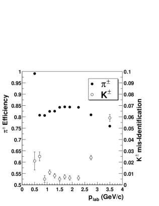
Figure 1: Pion selection performance as measured in data using $D^{*+}\rightarrow D^{0}\pi^{+},D^{0}\rightarrow K^{-}\pi^{+}$ decays as a function of momentum in the laboratory frame $p_{lab}$.

3.3 Reconstruction of $\rho/\omega$ Meson

The $\rho^{0}\rightarrow\pi^{+}\pi^{-}$ candidates are reconstructed by calculating a common vertex for two tracks of opposite charge. For the $\rho^{+}\rightarrow\pi^{+}\pi^{0}$ and $\omega\rightarrow\pi^{+}\pi^{-}\pi^{0}$ reconstruction, $\pi^{0}$ candidates are identified as two photon candidates reconstructed in the calorimeter each of with energy greater than $50\mathrm{\,Me\kern-1.00006ptV}$. The invariant mass of the pair is required to be $0.115<M_{\gamma\gamma}<0.150{\mathrm{\,Ge\kern-1.00006ptV\!/}c^{2}}$. A kinematic fit with $M_{\gamma\gamma}$ constrained to the nominal $\pi^{0}$ mass is used to improve the momentum resolution. The $\rho^{+}$ candidates result from $\pi^{0}$ candidates paired with an identified charged pion. The invariant mass $M_{\pi\pi}$ of the $\rho$ candidates is required to be between $0.520$ and $1.020{\mathrm{\,Ge\kern-1.00006ptV\!/}c^{2}}$. The $\omega$ candidates are reconstructed from combinations of oppositely charged identified pions with a successfully calculated vertex and $\pi^{0}$ candidates with invariant mass $0.7596<M_{\pi^{+}\pi^{-}\pi^{0}}<0.8056{\mathrm{\,Ge\kern-1.00006ptV\!/}c^{2}}$. The momentum of the candidate $\rho$ mesons, measured in the center of mass system must satisfy $2.3<p_{\rho}^{*}<2.85$ and the $\omega$ mesons must satisfy $2.4<p_{\omega}^{*}<2.8$. This cut, which has very high signal efficiency, is applied in order to reduce the number of events where more than one candidate satisfies all of the cuts.

3.4 Reconstruction of the $B$ Meson

The photon and $\rho/\omega$ meson candidate are combined to form the $B$ meson candidate. The kinematic properties of the $B$ meson are evaluated in the CMS using the variables $\Delta E^{*}=E^{*}_{B}-E_{beam}^{*}$ and the beam-energy substituted mass $\mbox{$m_{\rm ES}$}=\sqrt{E^{*2}_{beam}-\mbox{$\boldmath{\mathrm{p}^{\prime}}$}_{B}^{*2}},$ where $E_{beam}^{*}$ is the energy of the beam, $E^{*}_{B}=E^{*}_{\gamma}+E^{*}_{\rho/\omega}$ is the reconstructed energy of the $B$ meson candidate and ${\mathrm{p}^{\prime}}_{B}^{*}$ is its momentum. For the purposes of the $m_{\rm ES}$ calculation, ${\mathrm{p}^{\prime}}_{B}^{*}$ is modified by scaling the photon energy so as to make $E^{*}_{\gamma}+E^{*}_{\rho/\omega}-E_{beam}^{*}=0$, under the assumption that the resolution of the primary photon energy dominates the $\Delta E^{*}$ resolution. This procedure reduces the tail in the $m_{\rm ES}$ resolution that results from the asymmetric photon energy response in the EMC. The signal events have $\mbox{$m_{\rm ES}$}=m_{B}$ and $\Delta E^{*}=0$ up to the experimental resolution of $\sim 3{\mathrm{\,Me\kern-1.00006ptV\!/}c^{2}}$ dominated by the beam-energy spread in the former case, and $\sim 50\mathrm{\,Me\kern-1.00006ptV}$ dominated by the reconstructed photon energy resolution in the latter.

We consider candidates in the region $-0.3<\Delta E^{*}<0.3\mathrm{\,Ge\kern-1.00006ptV}$ and $5.2<\mbox{$m_{\rm ES}$}<5.29{\mathrm{\,Ge\kern-1.00006ptV\!/}c^{2}}$ and define a signal region of $-0.2<\Delta E^{*}<0.1\mathrm{\,Ge\kern-1.00006ptV}$ and $5.27<\mbox{$m_{\rm ES}$}<5.29{\mathrm{\,Ge\kern-1.00006ptV\!/}c^{2}}$. Selection criteria have been optimized for best $S^{2}/(S+B)$, where $S$ and $B$ are the expected signal and background yield assuming ${\cal B}[B^{0}\rightarrow\rho^{0}\gamma]={\cal B}[B^{0}\rightarrow\omega\gamma]=\frac{1}{2}{\cal B}[B^{+}\rightarrow\rho^{+}\gamma]=10^{-6}$ (as expected from isospin symmetry) without knowledge of the yield or distribution of events in the signal region. The signal region extends lower on the negative side of $\Delta E^{*}$ due to the asymmetric photon energy response in the calorimeter resulting from energy leakage. For the small fraction of events (2.8 % for $B^{0}\rightarrow\rho^{0}\gamma$ signal) in which more than one $B$ meson candidate satisfies all the cuts, the candidate with the smallest value of $|\Delta E^{*}|$ is selected.

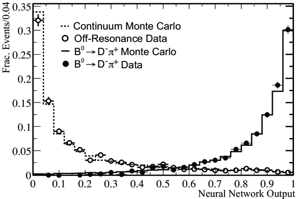
Figure 2: $B^{0}\rightarrow\rho^{0}\gamma$ neural network output for Monte Carlo-simulated events with comparison to data control samples.

3.5 Suppression of Background

The continuum and initial state radiation backgrounds are suppressed by a neural network that combines event topology variables into one discriminating variable [9]. The neural network responds non-linearly to the input variables and exploits correlations between the variables. The input variables are:

• $\cos{\theta^{*}_{T}}$, the cosine of the angle between the photon and the thrust axis of the rest of the event (excluding the $B$ meson candidate).

• $\cos{\theta^{*}_{B}}$, the cosine of the angle between the $B$ meson momentum and the beam axis.

• The energy flow in $10^{\circ}$ bins centered on the photon candidate momentum in the CMS.

• $\cos{\theta_{H}}$, the cosine of the helicity angle. For $B\rightarrow\rho\gamma$, we define $\theta_{H}$ as the angle between the $\pi^{+}$ momentum in the $\rho$ rest frame and the $\rho$ momentum in the $B$ meson rest frame. For $B^{0}\rightarrow\omega\gamma$, $\theta_{H}$ is defined as the angle between the normal to the plane defined by the $\pi^{+}\pi^{-}\pi^{0}$ momenta in the $\omega$ rest frame and the $\omega$ momentum in the $B$ meson rest frame. $\cos{\theta_{H}}$ should follow a $\sin^{2}\theta_{H}$ distribution for signal, while the continuum background is approximately flat.

• $R_{2}^{\prime}$, the ratio of second and zeroth order Fox-Wolfram moments in the frame recoiling from the photon momentum. This is effective against initial-state radiation, since in that frame the jet structure of the hadrons is recovered.

• The net flavor content, defined as $\sum_{i}|N^{+}_{i}-N^{-}_{i}|$, where $N^{\pm}_{i}$ are the number of $e^{\pm}$, $\mu^{\pm}$, $K^{\pm}$ and slow pions of each sign identified in the event.

• $|\Delta z|$, the vertex separation of the $B$ meson candidate and the rest of the event along the beam axis, is used for $B^{0}\rightarrow\rho^{0}\gamma$ and $B^{0}\rightarrow\omega\gamma$.

• $\cos\theta_{D}$, the cosine of the Dalitz angle of the $\omega$ decay is used for $B^{0}\rightarrow\omega\gamma$. $\cos\theta_{D}$ is defined as the angle between the. $\pi^{0}$ and the $\pi^{+}$ momenta in the rest frame of the $\pi^{+}\pi^{-}$ system. We expect $\cos\theta_{D}$ to be uniformly distributed for the combinatorial background and to follow a $\sin^{2}\theta_{D}$ distribution for true $\omega$ decays.

A separate neural network is trained for each mode using the back-propagation algorithm on samples of Monte Carlo-simulated signal and background. The output of the neural network, defined such that the signal processes peak at one and the continuum background at zero, is cross-checked on an independent sample of Monte Carlo-simulated events and data control samples for both the signal and background. The neural network output for $B^{0}\rightarrow\rho^{0}\gamma$ is shown in Figure 2, where the Monte Carlo simulation of the continuum background is compared with the off-resonance data and the output for Monte Carlo-simulated $B^{0}\rightarrow D^{-}\pi^{+}$ decays is compared with events reconstructed in the data. This latter check gives us confidence that the Monte Carlo simulates the $B\rightarrow\rho\gamma$ efficiency well, since most of the input variables of the neural network are not based on the properties of the signal decay itself, but rather on the properties of the other $B$ meson in the event.

We make a selection on the neural network output optimized for best $S^{2}/(S+B)$ for each mode. For $B^{+}\rightarrow\rho^{+}\gamma$, an additional requirement of $|\cos{\theta_{H}}|<0.6$ is made to reject $B^{+}\rightarrow\rho^{+}\pi^{0}$ events which have a $\cos^{2}\theta_{H}$ distribution, different from the expected $\sin^{2}\theta_{H}$ distribution from the signal process.

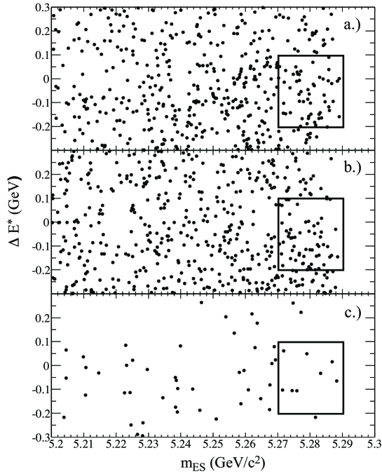
Figure 3: $\Delta E^{*}$ vs. $m_{\rm ES}$ for a.) $B^{0}\rightarrow\rho^{0}\gamma$, b.) $B^{+}\rightarrow\rho^{+}\gamma$ and c.) $B^{0}\rightarrow\omega\gamma$ candidates.

3.6 Background Estimation

Table 1 shows estimates for the expected background remaining in the signal region ($-0.2<\Delta E^{*}<0.1\mathrm{\,Ge\kern-1.00006ptV}$ and $\mbox{$m_{\rm ES}$}>5.27{\mathrm{\,Ge\kern-1.00006ptV\!/}c^{2}}$) after the neural network selection, using the off-resonance data for continuum and Monte Carlo simulation for $B\kern 1.79993pt\overline{\kern-1.79993ptB}{}$ backgrounds. There is good agreement between Monte Carlo estimates of continuum background and off-resonance data. The $B\kern 1.79993pt\overline{\kern-1.79993ptB}{}$ background is smaller than the continuum background.

	$B^{0}\rightarrow\rho^{0}\gamma$	$B^{+}\rightarrow\rho^{+}\gamma$	$B^{0}\rightarrow\omega\gamma$
	(Events)
Off-resonance data	$42.8\pm 7.0$	$66.5\pm 8.8$	$7.3\pm 3.3$
$uds+c\bar{c}+\tau^{+}\tau^{-}$ Monte Carlo	$39.8\pm 3.8$	$59.8\pm 4.6$	$8.4\pm 1.9$
$B\kern 1.79993pt\overline{\kern-1.79993ptB}{}$ Monte Carlo	$\;\>6.6\pm 1.0$	$12.2\pm 3.6$	$0.7\pm 0.3$
Signal Expectation	$\;\>9.9\pm 0.2$	$12.1\pm 0.3$	$3.4\pm 0.1$

Table 1: Estimates of continuum background (using both off-resonance data and Monte Carlo simulation), $B\kern 1.79993pt\overline{\kern-1.79993ptB}{}$ backgrounds and signal in the signal region. All estimates are scaled to a luminosity corresponding to 84 million $B\kern 1.79993pt\overline{\kern-1.79993ptB}{}$ pairs. Errors are statistical only.

3.7 Signal Extraction

After the neural network selection, the signal extraction in $B\rightarrow\rho\gamma$ is performed with an unbinned extended maximum likelihood fit in the variables $m_{\rm ES}$, $\Delta E^{*}$ and $M_{\pi\pi}$ with signal and continuum background components. Since the $B\kern 1.79993pt\overline{\kern-1.79993ptB}{}$ backgrounds are small relative to the continuum background, the signal extraction uses only a continuum component to describe the background. Biases due to $B\kern 1.79993pt\overline{\kern-1.79993ptB}{}$ backgrounds are estimated in the systematic studies described in Section 4. The signal $m_{\rm ES}$ and $\Delta E^{*}$ distributions are described by the Crystal Ball lineshape [11], with the exception of the $m_{\rm ES}$ distribution for $B^{0}\rightarrow\rho^{0}\gamma$, where the Gaussian distribution is used. Here, we expect the photon energy rescaling to eliminate the tail. The background $m_{\rm ES}$ and $\Delta E^{*}$ distributions are described by the ARGUS threshold function [12] and second order polynomial, respectively. For $B\rightarrow\rho\gamma$, the Breit-Wigner lineshape is used for the signal $M_{\pi\pi}$ distribution, while the background incorporates a sum of a resonant Breit-Wigner component and a continuum component described by a first order polynomial.

The parameters of the signal probability distributions are obtained from the Monte Carlo simulation and cross-checked in the data with the decays $B^{0}\rightarrow K^{*0}\gamma$, $K^{*0}\rightarrow K^{+}\pi^{-}$ for $B^{0}\rightarrow\rho^{0}\gamma$ and $B^{+}\rightarrow K^{*+}\gamma$, $K^{*+}\rightarrow K^{+}\pi^{0}$ for $B^{+}\rightarrow\rho^{+}\gamma$, which are topologically and kinematically similar. The parameters of the continuum background distributions are determined in the fit, with the exception of the fraction of the resonant $\rho\rightarrow\pi\pi$ contribution to the continuum $M_{\pi\pi}$ distribution, which is fixed to the value measured in the off-resonance data. In the $B^{0}\rightarrow\omega\gamma$, the signal extraction is performed in a similar fit to the $m_{\rm ES}$ and $\Delta E^{*}$ distributions; the $M_{\pi^{+}\pi^{-}\pi^{0}}$ distribution is not included in the fit, because the continuum background contains a large and uncertain fraction of true $\omega$ decays, which is difficult to model.

By inverting the pion selection on the charged pion (and selecting kaons) in the $B^{+}\rightarrow\rho^{+}\gamma$ analysis and on one of the charged pions in the $B^{0}\rightarrow\rho^{0}\gamma$ analysis, we obtain an orthogonal sample of events enhanced in the decays $B^{+}\rightarrow K^{*+}\gamma$, $K^{*+}\rightarrow K^{+}\pi^{0}$ and $B^{0}\rightarrow K^{*0}\gamma$, $K^{*0}\rightarrow K^{+}\pi^{-}$, respectively. The yield of $B\rightarrow K^{*}\gamma$ in these two samples is determined using the same fit procedure described for $B\rightarrow\rho\gamma$, with the expected signal distributions determined from Monte Carlo simulation. The resulting yields are in agreement with the expectations from previous measurements of ${\cal B}[B\rightarrow K^{*}\gamma]$ [10], as shown in Table 3, thus providing a cross-check on the event selection and signal extraction procedure up to the statistical uncertainty in the extracted yields and the uncertainties in the measured branching fractions.

The $\Delta E^{*}$ vs. $m_{\rm ES}$ distributions of the $B\rightarrow\rho\gamma$ and $B^{0}\rightarrow\omega\gamma$ candidates are shown in Figure 3 and the fitted yields summarized in Table 3. The quality of the fit is determined by comparing the minimum $-\log\mathcal{L}$ of the fit, where $\mathcal{L}$ is the overall likelihood of the fit, with values obtained from parameterized Monte Carlo simulation and found to be in good agreement.

Mode	Fitted Yield (Events)	Expected Yield (Events)
$B^{0}\rightarrow K^{*0}\gamma$	$343.2\pm 21.0$	$332\pm 36$
$B^{+}\rightarrow K^{*+}\gamma$	$\;\>93.1\pm 12.6$	$105\pm 18$

Table 2: The fitted yields in the $B\rightarrow K^{*}\gamma$-enhanced sample described in the text, and the expected yield from the measured branching fractions in [10].

Mode	Yield	$90\%$ C.L. Upper Limit Yield	Bias	Efficiency
	(Events)	(Events)	(Events)	$(\%)$
$B^{0}\rightarrow\rho^{0}\gamma$	$4.8\pm 5.2$	12.4	[-0.5,0.8]	12.3
$B^{+}\rightarrow\rho^{+}\gamma$	$6.2\pm 5.5$	15.4	[-0.1,2.0]	9.2
$B^{0}\rightarrow\omega\gamma$	$0.1\pm 2.3$	3.6	[-0.3,0.5]	4.6

Table 3: The fitted yields, the ranges of observed biases from $B\kern 1.79993pt\overline{\kern-1.79993ptB}{}$ backgrounds and selection efficiencies for $B^{0}\rightarrow\rho^{0}\gamma$, $B^{+}\rightarrow\rho^{+}\gamma$ and $B^{0}\rightarrow\omega\gamma$ in the on-resonance data sample. The efficiencies include the branching fractions for $\omega\rightarrow\pi^{+}\pi^{-}\pi^{0}$ (88.8%), $\rho^{0}\rightarrow\pi^{+}\pi^{-}$ ($\approx$ 99%) and $\rho^{+}\rightarrow\pi^{+}\pi^{0}$ ($\approx$ 100%).

4 Systematic Studies

The systematic uncertainties in this analysis are associated with uncertainties in the efficiency of the signal process reconstruction predicted by the Monte Carlo simulation and with the signal extraction procedure. Table 4 summarizes these uncertainties. The efficiency of the track selection is calculated by identifying tracks in the silicon vertex detector and evaluating the fraction that is well-reconstructed in the drift chamber. The pion identification efficiency in the DIRC is derived from a sample of $D^{*+}\rightarrow D^{0}\pi^{+},D^{0}\rightarrow K^{-}\pi^{+}$ decays. The photon and $\pi^{0}$ efficiencies are measured by comparing the ratio of events $N(\tau^{\pm}\rightarrow h^{\pm}\pi^{0})/N(\tau^{\pm}\rightarrow h^{\pm}\pi^{0}\pi^{0})$, where $h^{\pm}=\pi^{\pm},~{}K^{\pm}$, to the previously measured branching ratios [13]. The photon isolation and $\pi^{0}/\eta$ veto efficiency are dependent on the event multiplicity and are tested by “embedding” Monte Carlo-generated photons into both an exclusively reconstructed $B$ meson data sample and a generic $B\kern 1.79993pt\overline{\kern-1.79993ptB}{}$ Monte Carlo sample. The efficiencies of the neural network selection are compared between the exclusively reconstructed $B\rightarrow D\pi$ events in the data and the Monte Carlo simulation of both the $B\rightarrow D\pi$ and signal processes, and the observed variations taken as systematic uncertainties. The $M_{\pi^{+}\pi^{-}\pi^{0}}$ selection for the $B^{0}\rightarrow\omega\gamma$ is checked by comparing the resolution of the $\omega$ mass peak in the on-resonance data with the Monte Carlo simulation and evaluating the variation in efficiency.

Systematic uncertainties in the signal extraction procedure result from the modeling of the $B\kern 1.79993pt\overline{\kern-1.79993ptB}{}$ backgrounds and from uncertainties in the signal probability distribution functions used in the fit. The biases due to $B\kern 1.79993pt\overline{\kern-1.79993ptB}{}$ backgrounds are estimated by varying the distributions as well as the rates of the dominant backgrounds coming from $b\rightarrow s\gamma$ and $B^{+}\rightarrow\rho^{+}\pi^{0}$ decays. The full range of biases obtained from these variations is taken as the allowed range, as shown in the column labeled “Bias” in Table 3. The uncertainties resulting from the fixed parameters describing the signal distributions in the fit are estimated by varying the parameters within the uncertainty obtained from the analogous $B\rightarrow K^{*}\gamma$ processes in the data used to cross-check the expectations from the Monte Carlo simulation. The effects of these variations on the fitted signal yield in each mode is calculated and the range of observed biases are taken as systematic uncertainties in the signal yield.

	$B^{0}\rightarrow\rho^{0}\gamma$	$B^{+}\rightarrow\rho^{+}\gamma$	$B^{0}\rightarrow\omega\gamma$
	Systematic Uncertainty
Selection Criteria	$(\%)$	$(\%)$	$(\%)$
$B$ Count	1.1	1.1	1.1
$\gamma$ Eff.	1.5	1.5	1.5
$\pi^{0}$ Eff.	-	5.0	5.0
$\pi^{0}/\eta$ Veto	1.0	1.0	1.0
$\gamma$ Dist Cut	2.0	2.0	2.0
Tracking Eff.	2.5	1.3	2.4
$\pi$ Selection	6.0	3.0	6.0
$M_{\pi^{+}\pi^{-}\pi^{0}}$ Selection	-	-	2.0
Neural network Selection	8.0	6.0	14.0
Fit Distributions	5.0	10.0	5.0
Total	$11.8\%$	$13.4\%$	$17.3\%$

Table 4: Summary of systematic uncertainties for $B\rightarrow\rho\gamma$ and $B^{0}\rightarrow\omega\gamma$ expressed as percent error of the branching fraction.

5 Physics Results

Based on the observed signal yields we determine $90\%$ upper limits on the branching fraction by re-fitting the distributions with increasing fixed signal yields until the $-\log\mathcal{L}$ deviates by 0.82 relative to the minimum value. We correct for bias from $B\kern 1.79993pt\overline{\kern-1.79993ptB}{}$ backgrounds by applying the smallest observed bias to the signal yield (increasing the signal yield in all cases). The yield of events in the data sample are calculated with the Monte Carlo-derived efficiency lowered by one standard deviation in the systematic error. Finally, the estimated number of $B\kern 1.79993pt\overline{\kern-1.79993ptB}{}$ events in the sample is reduced by one standard deviation. The resulting preliminary $90\%$ confidence level upper limits for the branching fractions are ${\cal B}[B^{0}\rightarrow\rho^{0}\gamma]<1.4\times 10^{-6}$, ${\cal B}[B^{+}\rightarrow\rho^{+}\gamma]<2.3\times 10^{-6}$ and ${\cal B}[B^{0}\rightarrow\omega\gamma]<1.2\times 10^{-6}$.

For the purpose of comparing the limits to ${\cal B}[B\rightarrow K^{*}\gamma]$, we combine these limits into a single limit on the generic process $B\rightarrow\rho\gamma$ defined as

$${\cal B}[B\rightarrow\rho\gamma]\equiv{\cal B}[B^{+}\rightarrow\rho^{+}\gamma]=2\times{\cal B}[B^{0}\rightarrow\rho^{0}\gamma]=2\times{\cal B}[B^{0}\rightarrow\omega\gamma].$$

as expected from isospin symmetry. The resulting preliminary $90\%$ confidence level upper limit is
${\cal B}[B\rightarrow\rho\gamma]<1.9\times 10^{-6}$. Using the measured value of $\cal B$[$B\rightarrow K^{*}\gamma$] [10], this corresponds to a ratio of

$${\cal B}[B\rightarrow\rho\gamma]/{\cal B}[B\rightarrow K^{*}\gamma]<0.047.$$

We can convert this ratio to a limit on $|V_{td}/V_{ts}|$ using the following expression from [3].

$$\frac{{\cal B}[B\rightarrow\rho\gamma]}{{\cal B}[B\rightarrow K^{*}\gamma]}=\left|\frac{V_{td}}{V_{ts}}\right|^{2}\left(\frac{1-m_{\rho}^{2}/M_{B}^{2}}{1-m_{K^{*}}^{2}/M_{B}^{2}}\right)^{3}\zeta^{2}[1+\Delta R].$$

Taking the conservative limits of the two parameters, $\zeta=0.7$ and $\Delta R=-0.25$, we find
$|V_{td}/V_{ts}|<0.36$ at $90\%$ Confidence Level.

6 Summary

In conclusion, we have found no evidence for the exclusive $b\rightarrow d\gamma$ transitions $B\rightarrow\rho\gamma$ and $B^{0}\rightarrow\omega\gamma$ in 84 million $B\kern 1.79993pt\overline{\kern-1.79993ptB}{}$ decays studied with the BABAR detector. The preliminary $90\%$ confidence level upper limits on the branching fractions are significantly improved and within a factor of two of the largest Standard Model predictions, which indicate a range ${\cal B}[B^{+}\rightarrow\rho^{+}\gamma]=(0.9-1.5)\times 10^{-6}$.

7 Acknowledgments

We are grateful for the extraordinary contributions of our PEP-II colleagues in achieving the excellent luminosity and machine conditions that have made this work possible. The success of this project also relies critically on the expertise and dedication of the computing organizations that support BABAR. The collaborating institutions wish to thank SLAC for its support and the kind hospitality extended to them. This work is supported by the US Department of Energy and National Science Foundation, the Natural Sciences and Engineering Research Council (Canada), Institute of High Energy Physics (China), the Commissariat à l’Energie Atomique and Institut National de Physique Nucléaire et de Physique des Particules (France), the Bundesministerium für Bildung und Forschung and Deutsche Forschungsgemeinschaft (Germany), the Istituto Nazionale di Fisica Nucleare (Italy), the Research Council of Norway, the Ministry of Science and Technology of the Russian Federation, and the Particle Physics and Astronomy Research Council (United Kingdom). Individuals have received support from the A. P. Sloan Foundation, the Research Corporation, and the Alexander von Humboldt Foundation.

References

- [1] See for example, S. Bertolini, F. Borzumati and A. Masiero, Nucl. Phys. B 294, 321 (1987); H. Baer, M. Brhlik, Phys. Rev. D 55, 3201 (1997); J. Hewett and J. Wells, Phys. Rev. D 55, 5549 (1997); M. Carena et al., Phys. Lett. B 499, 141 (2001).
- [2] M. Beneke, T. Feldmann and D. Seidel, Nucl. Phys. B 612, 25 (2001); S. W. Bosch and G. Buchalla, Nucl. Phys. B 621, 459 (2002).
- [3] A. Ali and A. Y. Parkhomenko, Eur. Phys. J. C 23, 89 (2002).
- [4] B. Grinstein and D. Pirjol, Phys. Rev. D 62, 093002 (2000).
- [5] CLEO Collaboration, T.E. Coan et al., Phys. Rev. Lett. 84, 5283 (2000); BELLE Collaboration, Y. Ushiroda et al., contributed to BCP4, Ago Town, Japan, Feb 2001. hep-ex/0104045.
- [6] BABAR Collaboration, B. Aubert et al., Nucl. Instrum. Meth. A 479, 1 (2002).
- [7] PEP-II Conceptual Design Report, SLAC-0418 (1993).
- [8] Geant4 Collaboration, “Geant4 - A Simulation ToolKit”, CERN-IT-2002-003. To be published in Nucl. Instrum. Meth. A.
-
[9]
We use the Stuttgart Neural Network Simulator:
http://www-ra.informatik.uni-tuebingen.de/SNNS - [10] BABAR Collaboration, B. Aubert et al., Phys. Rev. Lett. 88, 101805 (2002).
- [11] The “Crystal Ball” lineshape is a modified Gaussian distribution with a transition to a tail function on one side: for and for where and are defined such as to maintain continuity of the function and its first derivative.
- [12] We use the distribution , where , to describe the background distribution. The function was introduced by the ARGUS collaboration; H.Albrecht et al., Z. Phys. C 48, 543 (1990)
- [13] CLEO Collaboration, M. Procario et al., Phys. Rev. Lett. 70, 1207 (1993).