The BABAR Collaboration

July 24, 2002

We measure the $B^{0}$ lifetime $\tau_{B^{0}}$ and the $B^{0}$-$\kern 1.79993pt\overline{\kern-1.79993ptB}{}^{0}$ oscillation frequency $\Delta m_{d}$ with a sample of approximately 14,000 exclusively reconstructed $B^{0}\rightarrow D^{*-}\ell^{+}\nu_{\ell}$ signal events, selected from 23 million $B\overline{B}$ pairs recorded at the $\Upsilon(4S)$ resonance with the BABAR detector at the Stanford Linear Accelerator Center. The $b$-quark flavor of the other $B$ at the time of decay and its decay position are determined inclusively. The lifetime and oscillation frequency are measured simultaneously with an unbinned maximum-likelihood fit that uses, for each event, the measured difference in $B$ decay times ($\Delta t$), the calculated uncertainty on $\Delta t$, the signal and background probabilities, and $b$-quark tagging information for the other $B$. The preliminary results are

$$\tau_{B^{0}}=(1.523^{+0.024}_{-0.023}\pm 0.022)~{}\rm{ps}$$

and

$$\Delta m_{d}=(0.492\pm 0.018\pm 0.013)~{}\rm{ps}^{-1}.$$

The statistical correlation coefficient between $\tau_{B^{0}}$ and $\Delta m_{d}$ is $-0.22$.

1 Introduction and analysis overview

The time evolution of $B^{0}$ mesons is governed by the overall decay rate $1/\tau_{B^{0}}$ and the $B^{0}$-$\kern 1.79993pt\overline{\kern-1.79993ptB}{}^{0}$ oscillation frequency $\Delta m_{d}$. The phenomenon of particle-antiparticle oscillations or “mixing” has been observed in neutral mesons containing a down quark and a strange quark ($K$ mesons) or a bottom quark ($B$ mesons) [1]. In the Standard Model of particle physics, $B$ mixing is the result of second-order charged weak interactions involving box diagrams containing virtual quarks with charge $2/3$. In $B$ mixing, the diagram containing the top quark dominates. Therefore, the mixing frequency $\Delta m_{d}$ is sensitive to the Cabibbo-Kobayashi-Maskawa quark-mixing matrix element $V_{td}$ [2]. In the neutral $K$ meson system, mixing also has contributions from real intermediate states accessible to both a $K^{0}$ and a $\kern 1.79993pt\overline{\kern-1.79993ptK}{}^{0}$ meson. These contributions are expected to be small for $B$ mixing and are assumed to be negligible in this analysis.

We present a measurement of the $B^{0}$ lifetime $\tau_{B^{0}}$ and the oscillation frequency $\Delta m_{d}$ based on a sample of $\approx$14,000 exclusively reconstructed $B^{0}\rightarrow D^{*-}\ell^{+}\nu_{\ell}$ decays selected from a sample of 23 million $B\overline{B}$ events recorded at the $\Upsilon(4S)$ resonance with the BABAR detector at the Stanford Linear Accelerator Center, in 1999-2000. In this experiment, 9 GeV electrons and 3.1 GeV positrons, circulating in the PEP-II storage ring, annihilate to produce $B\overline{B}$ pairs moving along the $e^{-}$ beam direction ($z$ axis) with a known Lorentz boost of $\beta\gamma=0.55$, which allows a measurement of the time between the two $B$ decays, $\Delta t$.

The proper decay-time difference $\Delta t$ between two neutral $B$ mesons produced in a coherent $P$-wave state in an $\Upsilon(4S)$ event is governed by the following probabilities to observe an unmixed event,

$$P(B^{0}\kern 1.79993pt\overline{\kern-1.79993ptB}{}^{0}\rightarrow B^{0}\kern 1.79993pt\overline{\kern-1.79993ptB}{}^{0})\propto e^{-|\Delta t|/\tau_{B^{0}}}(1+\cos\Delta m_{d}\Delta t),$$ (1)

or a mixed event,

$$P(B^{0}\kern 1.79993pt\overline{\kern-1.79993ptB}{}^{0}\rightarrow B^{0}B^{0}\ {\rm or}\ \kern 1.79993pt\overline{\kern-1.79993ptB}{}^{0}\kern 1.79993pt\overline{\kern-1.79993ptB}{}^{0})\propto e^{-|\Delta t|/\tau_{B^{0}}}(1-\cos\Delta m_{d}\Delta t).$$ (2)

Therefore, if we measure $\Delta t$ and identify the $b$-quark flavor of both $B$ mesons at their time of decay, we can extract the $B^{0}$ lifetime $\tau_{B^{0}}$ and the mixing frequency $\Delta m_{d}$. In this analysis, one $B$ is reconstructed in the mode $B^{0}\rightarrow D^{*-}\ell^{+}\nu_{\ell}$, which has a measured branching fraction of $(4.60\pm 0.21)\%$ [3]. Although the neutrino cannot be detected, the requirement of a reconstructed $D^{*-}\rightarrow\overline{D}^{0}\pi^{-}$ decay and a high-momentum lepton satisfying kinematic constraints consistent with the decay $B^{0}\rightarrow D^{*-}\ell^{+}\nu_{\ell}$ allows the isolation of a signal sample with (65 - 89)% purity, depending on the $D^{0}$ decay mode and whether the lepton candidate is an electron or a muon. The charges of the final-state particles identify the meson as a $B^{0}$ or a $\kern 1.79993pt\overline{\kern-1.79993ptB}{}^{0}$. The remaining charged particles in the event, which originate from the other $B$ (referred to as $B_{\rm tag}$), are used to identify, or “tag”, its flavor as a $B^{0}$ or a $\kern 1.79993pt\overline{\kern-1.79993ptB}{}^{0}$. The time difference $\Delta t=t_{D^{*}\ell}-t_{\rm tag}\approx\Delta z/\beta\gamma c$ is determined from the separation $\Delta z$ of the decay vertices for the $D^{*-}\ell^{+}$ candidate and the tagging $B$ along the boost direction. The average separation is 250 $\mu$m.

The oscillation frequency $\Delta m_{d}$ and the average lifetime of the neutral $B$ meson, $\tau_{B^{0}}$, are determined simultaneously with an unbinned maximum-likelihood fit to the measured $\Delta t$ distributions of events that are classified as mixed and unmixed. This is in contrast to published measurements in which only $\Delta m_{d}$ is measured with $\tau_{B^{0}}$ fixed to the world average, or only $\tau_{B^{0}}$ is measured. There are several reasons to measure the lifetime and oscillation frequency simultaneously. The statistical precision for both $\tau_{B^{0}}$ and $\Delta m_{d}$ is comparable to the uncertainty on the world average. Therefore, it is appropriate to measure both quantities rather than fixing the lifetime to the world average. Since mixed and unmixed events have different $\Delta t$ distributions, the mixing information for each event gives greater sensitivity to the $\Delta t$ resolution function and a smaller statistical uncertainty on $\tau_{B^{0}}$. Also, since $B^{+}B^{-}$ events do not mix, we can use the $\Delta t$ distributions for mixed and unmixed events to help discriminate between $B^{0}\kern 1.79993pt\overline{\kern-1.79993ptB}{}^{0}$ signal events and $B^{+}B^{-}$ background events in the lifetime and mixing measurement.

There are three main experimental complications that affect the $\Delta t$ distributions given in Eqs. 1 and 2. First, the tagging algorithm, which classifies events into categories $c$ depending on the source of the available tagging information, incorrectly identifies the flavor of $B_{\rm tag}$ with a probability $w_{c}$ with a consequent reduction of the observed amplitude for the mixing oscillation by a factor $(1-2w_{c})$. Second, the resolution for $\Delta t$ is comparable to the lifetime and must be well understood. The probability density functions (PDF’s) for the unmixed ($+$) and mixed ($-$) signal events can be expressed as the convolution of the underlying ${\Delta t}_{\rm true}$ distribution for tagging category $c$,

$${e^{-|{\Delta t}_{\rm true}|/\tau_{B^{0}}}\over 4\tau_{B^{0}}}[1\pm(1-2w_{c})\cos\Delta m_{d}{\Delta t}_{\rm true}],$$

with a resolution function ${\cal R}({\Delta t}_{\rm meas}-{\Delta t}_{\rm true};\vec{q}_{c})$ that depends on a set of parameters $\vec{q}_{c}$. A final complication is that the sample of selected $B^{0}\rightarrow D^{*-}\ell^{+}\nu_{\ell}$ candidates is not pure signal.

To characterize the backgrounds, we select control samples of events enhanced in each type of background and determine the signal and background probabilities for each event in the signal and background control samples as described in Sec. 4. The measurement of $\Delta z$ and the determination of $\Delta t$ and $\sigma_{\Delta t}$ for each event is discussed in Sec. 5. The $b$-quark tagging algorithm is described in Sec. 6. In Sec. 7, we describe the unbinned maximum-likelihood fit. The physics model and $\Delta t$ resolution function used to describe the measured $\Delta t$ distribution for signal are given in Sec. 8. A combination of Monte Carlo simulation and data samples are used to determine the parameterization of the PDF’s to describe the $\Delta t$ distribution for each type of background, as described in Sec. 9. The likelihood is maximized in a simultaneous fit to the signal and background control samples to extract the $B^{0}$ lifetime $\tau_{B^{0}}$, the mixing frequency $\Delta m_{d}$, the mistag probabilities $w_{c}$, the signal $\Delta t$ resolution parameters $\vec{q}_{c}$, the background $\Delta t$ model parameters, and the fraction of $B^{+}\rightarrow D^{*-}\ell^{+}\nu_{\ell}X$ decays in the signal sample. The results of the fit are given in Sec. 10. Cross-checks are described in Sec. 11 and systematic uncertainties are summarized in Sec. 12.

2 The BABAR detector

The BABAR detector is described in detail elsewhere [4]. The momenta of charged particles are measured with a combination of a 40-layer drift chamber (DCH) and a five-layer silicon vertex tracker (SVT) in a 1.5-T solenoidal magnetic field. A detector of internally-reflected Cherenkov radiation (DIRC) is used for charged hadron identification. Kaons are identified with a neural network based on the likelihood ratios calculated from d$E$/d$x$ measurements in the SVT and DCH, and from the observed pattern of Cherenkov light in the DIRC. A finely-segmented CsI(Tl) electromagnetic calorimeter (EMC) is used to detect photons and neutral hadrons, and to identify electrons. Electron candidates are required to have a ratio of EMC energy to track momentum, an EMC cluster shape, DCH d$E$/d$x$, and DIRC Cherenkov angle all consistent with the electron hypothesis. The instrumented flux return (IFR) contains resistive plate chambers for muon and long-lived neutral hadron identification. Muon candidates are required to have IFR hits located along the extrapolated DCH track, an IFR penetration length, and an energy deposit in the EMC consistent with the muon hypothesis.

3 Data samples

The data used in this analysis were recorded with the BABAR detector [4] at the PEP-II storage ring [5] in the period October 1999 to December 2000. The total integrated luminosity of the data set is 20.6 fb^-1 collected at the $\Upsilon(4S)$ resonance and 2.6 fb^-1 collected about 40 MeV below the $\Upsilon(4S)$ (off-resonance data). The corresponding number of produced $B\overline{B}$ pairs is 23 million.

Samples of Monte-Carlo simulated $B\overline{B}$ and $c\overline{c}$ events, generated with a GEANT3 [6] detector simulation, are analyzed through the same analysis chain as the real data to check for biases in the extracted physics parameters and are also used to develop models for describing detector resolution effects. The values of the parameters used in these models are determined with real data. The equivalent luminosity of this simulated data is approximately equal to that of the real data for $B\overline{B}$ events and about half that of real data for $c\overline{c}$ events. In addition, we generate signal Monte Carlo samples in which one neutral $B$ meson in every event decays to $D^{*-}\ell^{+}\nu_{\ell}$, with $D^{*-}\rightarrow\kern 1.79993pt\overline{\kern-1.79993ptD}{}^{0}\pi^{-}$, and the other neutral $B$ meson decays generically. The $D^{0}$ then decays to one of the four final states reconstructed in this analysis (described in the next section). The equivalent luminosity of the simulated signal samples is equal to approximately 2 to 8 times that of the real data, depending on the $D^{0}$ decay mode.

4 Event selection and characterization

We select events containing a fully-reconstructed $D^{*-}$ and an identified oppositely-charged electron or muon. This $D^{*-}\ell^{+}$ pair is then required to pass kinematic cuts that enhance the contribution of semileptonic $B^{0}\rightarrow D^{*-}\ell^{+}\nu_{\ell}$ decays. In addition to the signal sample, we select several control samples that are used to characterize the main sources of background.

We define the following classification of the sources of signal and background that we expect to contribute to this sample. The nomenclature shown in italics will be used throughout this paper to define signal and all possible types of background.

1. Events with a correctly reconstructed $D^{*-}$ candidate:

   1. Events that originate from $B\overline{B}$ events:

      1. Events with a correctly identified lepton candidate:

         1. Signal – $B^{0}\rightarrow D^{*-}\ell^{+}\nu_{\ell}$ (X) decays.

         2. Uncorrelated-lepton background – ($B\rightarrow D^{*-}X,\ {\rm other}\ {B}\rightarrow\ell^{+}X$) or ($B\rightarrow D^{*-}X,\ X\rightarrow\ell^{+}Y$)

         3. Charged $B$ background – $B^{+}\rightarrow D^{*-}\ell^{+}\nu_{\ell}X$.

      2. Fake-lepton background – events with a misidentified lepton candidate.

   2. Continuum background – $c\overline{c}\rightarrow D^{*-}X$.

2. Combinatoric background – events with a misreconstructed $D^{*-}$ candidate.

Lepton candidates are defined as charged tracks with momentum in the $\Upsilon(4S)$  rest frame greater than 1.2 GeV. For the $D^{*-}e^{+}$ samples, the electron candidate passes selection criteria with a corresponding electron identification efficiency of about 90% and hadron misidentification less than 0.2%. For the $D^{*-}\mu^{+}$ samples, the muon candidate passes selection criteria with a corresponding muon identification efficiency of about 70% and hadron misidentification between 2% and 3%. For the fake-lepton control sample, $D^{*-}\ell^{+}$ candidates are accepted if the lepton fails both electron and muon selection criteria looser than those required for lepton candidates.

$D^{*}$ candidates are selected in the decay mode $D^{*-}\rightarrow\kern 1.79993pt\overline{\kern-1.79993ptD}{}^{0}\pi^{-}$. The $D^{0}$ candidate is reconstructed in the modes $K^{-}\pi^{+}$, $K^{-}\pi^{+}\pi^{-}\pi^{+}$, $K^{-}\pi^{+}\pi^{0}$ and $K^{0}_{S}\pi^{-}\pi^{+}$. The daughters of the $D^{0}$ decay are selected according to the following definitions. $\pi^{0}$ candidates are reconstructed from two photons with invariant mass within 15.75 MeV of the $\pi^{0}$ mass. The mass of the photon pair is constrained to the $\pi^{0}$ mass and the photon pair is kept as a $\pi^{0}$ candidate if the $\chi^{2}$ probability of the fit is greater than 1%. $K^{0}_{S}$ candidates are reconstructed from a pair of charged particles with invariant mass within 15 MeV of the $K^{0}_{S}$ mass. The pair of tracks is retained as a $K^{0}_{S}$ candidate if the $\chi^{2}$ probability that the two tracks form a common vertex is greater than 1%. Charged kaon candidates satisfy loose kaon criteria for the $K^{-}\pi^{+}$ mode and tighter criteria for the $K^{-}\pi^{+}\pi^{-}\pi^{+}$ and $K^{-}\pi^{+}\pi^{0}$ modes. For the $K^{-}\pi^{+}\pi^{0}$ and $K^{0}_{S}\pi^{-}\pi^{+}$ modes, a likelihood is calculated as the square of the decay amplitude in the Dalitz plot for the three-body candidate, based on measured amplitudes and phases [7]. The candidate is retained if the likelihood is greater than 10% of its maximum value across the Dalitz plot.

$D^{0}$ candidates have measured invariant mass within 17 MeV of the $D^{0}$ mass for the $K^{-}\pi^{+}$, $K^{-}\pi^{+}\pi^{-}\pi^{+}$, and $K^{0}_{S}\pi^{-}\pi^{+}$ modes, and within 34 MeV for the $K^{-}\pi^{+}\pi^{0}$ mode. The invariant mass of the daughters is constrained to the $D^{0}$ mass and the tracks are constrained to a common vertex in a simultaneous fit. The $D^{0}$ candidate is retained if the $\chi^{2}$ of the fit is greater than 0.1%.

The low-momentum pion candidates for the $D^{*-}\rightarrow\kern 1.79993pt\overline{\kern-1.79993ptD}{}^{0}\pi^{-}$ decay are selected with total momentum less than 450 MeV in the $\Upsilon(4S)$ rest frame and momentum transverse to the beamline greater than 50 MeV. The momentum of the $D^{*}$ candidate in the $\Upsilon(4S)$ rest frame is between 0.5 and 2.5 GeV. The $D^{*-}\ell^{+}$ candidate satisfies $|\cos\theta^{*}_{\rm thrust}|<0.85$, where $\theta^{*}_{\rm thrust}$ is the angle between the thrust axis of the $D^{*-}\ell^{+}$ candidate and the thrust axis of the remaining charged and neutral particles in the event. $D^{*-}\ell^{+}$ candidates are retained if the $\chi^{2}$  probability that the daughter tracks form a common vertex is greater than 1% and $m(D^{*})-m(D^{0})$ is less than 165 MeV, where $m(D^{*})$ is the candidate $\kern 1.79993pt\overline{\kern-1.79993ptD}{}^{0}\pi^{-}$ mass calculated with the candidate $\kern 1.79993pt\overline{\kern-1.79993ptD}{}^{0}$ mass constrained to the true $D^{0}$ mass, $m(D^{0})$.

We define two angular quantities for each $D^{*-}\ell^{+}$ candidate to classify them into a sample enriched in $B^{0}\rightarrow D^{*-}\ell^{+}\nu_{\ell}$ signal events, in which the $D^{*}$ and lepton candidates are on opposite sides of the event, and a sample enriched in uncorrelated-lepton background events, in which the $D^{*}$ and lepton candidates are on the same side of the event. The first angle is $\theta_{D^{*},\ell}$, the angle between the $D^{*}$ and lepton candidates in the $\Upsilon(4S)$ rest frame. The second angle is $\theta_{B,D^{*}\ell}$, the angle between the direction of the $B^{0}$ and the vector sum of the $D^{*}$ and lepton candidate momenta, calculated in the $\Upsilon(4S)$ rest frame. Since we do not know the direction of the $B^{0}$, we calculate the cosine of $\theta_{B,D^{*}\ell}$ from the following equation, in which we assume that the only $B$ decay particle missed in the reconstruction is a massless neutrino:

$$\cos\theta_{B,D^{*}\ell}\equiv{-(m^{2}_{B^{0}}+m^{2}_{D^{*}\ell}-2E_{B}E_{D^{*}\ell})\over 2|\vec{p}_{B}||\vec{p}_{D^{*}\ell}|}.$$ (3)

All quantities in Eq. 3 are defined in the $\Upsilon(4S)$ rest frame. The energy and the magnitude of the momentum of the $B$ are calculated from the $e^{+}e^{-}$ center-of-mass energy and the $B^{0}$ mass. For true $B^{0}\rightarrow D^{*-}\ell^{+}\nu_{\ell}$ events, $\cos\theta_{B,D^{*}\ell}$ lies in the physical region $[-1,+1]$, except for detector resolution effects. Backgrounds lie inside and outside the range $[-1,+1]$. We also calculate the same angle with the lepton momentum direction reflected through the origin in the $\Upsilon(4S)$ rest frame: $\theta_{B,D^{*}(-\ell)}$.

A sample enhanced in $B^{0}\rightarrow D^{*-}\ell^{+}\nu_{\ell}$ signal events (called the opposite-side sample) is composed of $D^{*-}\ell^{+}$ candidates with $\cos\theta_{D^{*}\ell}<0$ and $|\cos\theta_{B,D^{*}\ell}|<1.1$. Samples are defined for lepton candidates that satisfy the criteria for an electron, a muon and a fake-lepton. The first two samples are the signal samples, and the latter is the fake-lepton control sample.

An additional background control sample, representative of the uncorrelated-lepton background and called the same-side sample, is composed of $D^{*-}\ell^{+}$ candidates satisfying $\cos\theta_{D^{*}\ell}\geq 0$ and $|\cos\theta_{B,D^{*}(-\ell)}|<1.1$. We use $\cos\theta_{B,D^{*}(-\ell)}$ rather than $\cos\theta_{B,D^{*}\ell}$ because, in Monte Carlo simulation, the distribution of $\cos\theta_{B,D^{*}(-\ell)}$ in this control sample is similar to the distribution of $\cos\theta_{B,D^{*}\ell}$ for uncorrelated-lepton background in the signal sample, whereas the distribution of $\cos\theta_{B,D^{*}\ell}$ in the background control sample is systematically different.

$D^{*-}\ell^{+}$ candidates are retained if a fit of the lepton, $\pi^{-}$, and $D^{0}$ candidates to a common vertex converges. In addition, several criteria that depend on the charged tracks in the rest of the event, as well as the $D^{*-}\ell^{+}$ candidate, are applied. Events are retained if at least two tracks are used to determine the decay point of the other $B$, the fit that determines the distance $\Delta z$ between the two $B$ decays along the beamline converges, the time between decays ($\Delta t$) calculated from $\Delta z$ is less than 18 ps, and the calculated error on $\Delta t$ ($\sigma_{\Delta t}$) is less than 1.8 ps.

Approximately $68,000$ candidates pass the above selection criteria. These candidates are distributed over two signal samples and ten background control samples defined by the following characteristics: whether the data was recorded on or off the $\Upsilon(4S)$ resonance (two choices); whether the candidate lepton is same-side or opposite-side to the $D^{*}$  candidate (two choices); and whether the lepton candidate passes the criteria for an electron, a muon, or a fake lepton (three choices).

The combinatoric background due to events with a misreconstructed $D^{*}$  candidate can be distinguished from events with a real $D^{*}$ in a plot of the mass difference $m(D^{*})-m(D^{0})$. The $m(D^{*})-m(D^{0})$ distributions for the samples of signal events (opposite-side $D^{*-}e^{+}$ and $D^{*-}\mu^{+}$ candidates in on-resonance data) are shown as data points in Fig. 1 for electron candidates (left) and muon candidates (right).

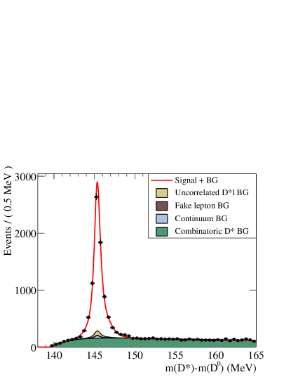
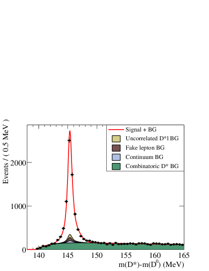
Figure 1: $m(D^{*})-m(D^{0})$ distribution for events passing all selection criteria for $B^{0}\rightarrow D^{*-}\ell^{+}\nu_{\ell}$, with an electron (left) or muon (right) candidate. The points correspond to the data. The curve is the result of a simultaneous unbinned maximum likelihood fit to this sample of events and a number of background control samples. The shaded distributions correspond to the four types of background described in the text.

Each of the 12 samples described above are further divided into 30 subsamples according to the following characteristics that may affect the $m(D^{*})-m(D^{0})$ or $\Delta t$  distributions.

1. The $\pi^{-}$ from the $D^{*}$ decay reconstructed in the SVT only, or in the SVT and DCH (two choices): The $m(D^{*})-m(D^{0})$ resolution is worse when the $\pi^{-}$ is reconstructed only in the SVT.

2. The $D^{0}$ candidate reconstructed in the mode $K^{-}\pi^{+}$ or $K^{-}\pi^{+}\pi^{0}$ or ($K^{-}\pi^{+}\pi^{-}\pi^{+}$ or $K^{0}_{S}\pi^{-}\pi^{+}$) (three choices): The level of contamination from combinatoric background and the $m(D^{*})-m(D^{0})$ resolution may depend on the $D^{0}$ decay mode.

3. The $b$-tagging information used for the other $B$ (five choices; see Sec. 6): The level of contamination from each type of background and the $\Delta t$ resolution parameters may depend on the tagging information.

This allows subdivision into 360 samples. In the unbinned maximum likelihood fits to the $m(D^{*})-m(D^{0})$ and ($\Delta t$, $\sigma_{\Delta t}$) distributions, individual fit parameters are shared among different sets of subsamples based on physics motivation and observations in the data.

We do a simultaneous fit to the $m(D^{*})-m(D^{0})$ distributions for all 360 subsamples. The peak due to real $D^{*}$ candidates is modeled by the sum of two Gaussian distributions; the mean and variance of both the Gaussian distributions, as well as the relative normalization of the two Gaussians, are free parameters in the fit. We model the shape of the combinatoric background with the function

$${1\over N}\left[1-\exp\left(-{\delta m-\delta m_{0}\over c_{1}}\right)\right]\left({\delta m\over\delta m_{0}}\right)^{c_{2}},$$ (4)

where $\delta m\equiv m(D^{*})-m(D^{0})$, $N$ is a normalization constant, $\delta m_{0}$ is a kinematic threshold equal to the mass of the $\pi^{-}$, and $c_{1}$ and $c_{2}$ are free parameters in the fit. An initial fit is done to determine the shape parameters describing the peak and combinatoric background. Separate values of the five parameters describing the shape of the peak are used for the six subsamples defined by whether the $\pi^{-}$ candidate is tracked in the SVT only or in the SVT and DCH, and the three types of $D^{0}$ decay modes. Each of these six groups that share peak parameters is further subdivided into twelve subgroups that each share a common set of the two combinatoric background shape parameters. Ten of these twelve subgroups are defined by the five tagging categories for the large signal samples and for the fake-lepton control samples, in on-resonance data. The other two subgroups are defined as same-side, on-resonance samples and all off-resonance samples.

Once the peak and combinatoric background shape parameters have been determined, we fix the shape parameters and determine the peak and combinatoric background yields in each of the 360 subsamples with an unbinned extended maximum-likelihood fit. The total peak yields in the signal sample and each background control sample are then used to determine the amount of true signal and each type of peaking background in the $m(D^{*})-m(D^{0})$ peak of each sample as follows.

1. Fake-lepton background –   Particle identification and misidentification efficiencies for the electron, muon, and fake-lepton selection criteria are measured in data as a function of laboratory momentum, polar angle, and azimuthal angle, for true electrons, muons, pions, kaons, and protons. $B^{0}\kern 1.79993pt\overline{\kern-1.79993ptB}{}^{0}$ and $B^{+}B^{-}$ Monte Carlo simulations are used to determine the measured laboratory momentum, polar angle, and azimuthal angle distributions for true electrons, muons, pions, kaons and protons that pass all selection criteria for $D^{*-}\ell^{+}$ candidates, except the lepton (or fake-lepton) identification criteria. These distributions are combined with the measured particle identification efficiencies and misidentification probabilities to determine the momentum- and angle-weighted probabilities for a true lepton or true hadron to pass the criteria for a lepton or a fake lepton in each of the $D^{*-}\ell^{+}$ signal and background control samples. We then use these efficiencies and misidentification probabilities, and the observed number of lepton and fake-lepton candidates in data, to determine the number of true leptons and fake leptons (hadrons) in each control sample.

2. Uncorrelated-lepton background –  To determine the number of uncorrelated-lepton events in each sample, we use the relative efficiencies from Monte Carlo simulation for signal and uncorrelated-lepton events to pass the criteria for same-side and opposite-side samples.

3. Continuum background –  We use the peak yields in off-resonance data, scaled by the relative integrated luminosity for on- and off-resonance data, to determine the continuum-background yields in on-resonance data.

The peak yields and continuum, fake-lepton, and uncorrelated-lepton fractions of the peak yield, as well as the combinatoric fraction of all events in a $m(D^{*})-m(D^{0})$  signal window, are shown in Table 1 for the signal and background control samples in on-resonance data. The peak yields include the peaking backgrounds. The signal window is defined as (143 - 148) MeV for the calculation of combinatoric background fractions.

Table 1: Peak yields and continuum, fake-lepton, and uncorrelated-lepton fractions of the peak yield, and the combinatoric fraction of total events in a $m(D^{*})-m(D^{0})$  signal window for the signal and background control samples in on-resonance data. Peak yields include the peaking backgrounds. The signal window for combinatoric background fractions is defined as (143 - 148) MeV. OS and SS refer to opposite-side and same-side samples; $e$, $\mu$, and f indicate the type of lepton candidate: electron, muon or fake-lepton.

Category		Peak Yield	$f_{\mathrm{cont}}(\%)$	$f_{\mathrm{fake}}(\%)$	$f_{\mathrm{uncorr}}(\%)$	$f_{\mathrm{comb}}(\%)$
OS	$e$	$7008\pm 91$	$1.53\pm 0.42$	$0.1678\pm 0.0042$	$3.14\pm 0.39$	$17.89\pm 0.24$
	$\mu$	$6569\pm 88$	$2.27\pm 0.57$	$2.669\pm 0.067$	$2.85\pm 0.48$	$18.36\pm 0.25$
	f	$8770\pm 108$	$12.8\pm 1.3$	$72.4\pm 1.8$	$0.7\pm 1.6$	$31.40\pm 0.24$
SS	$e$	$306\pm 21$	$0.000\pm 0.006$	$0.533\pm 0.039$	$56.9\pm 7.0$	$34.0\pm 1.3$
	$\mu$	$299\pm 20$	$5.1\pm 3.6$	$8.89\pm 0.64$	$48.9\pm 8.0$	$34.4\pm 1.3$
	f	$1350\pm 45$	$20.4\pm 4.1$	$74.4\pm 5.4$	$3.6\pm 7.8$	$42.59\pm 0.61$

Finally, we use the calculated fractions and fitted shapes of the background sources in each control sample to estimate the probability of each candidate to be due to signal or each type of background (combinatoric, continuum, fake-lepton, or uncorrelated-lepton) when we fit the ($\Delta t$, $\sigma_{\Delta t}$) distribution to determine the lifetime and mixing parameters. We take advantage of the fact that charged and neutral $B$ decays have different decay-time distributions (because the charged $B$ does not mix) to determine the fraction of charged $B$ background events in the fit to ($\Delta t$, $\sigma_{\Delta t}$).

5 Decay-time measurement

The decay-time difference $\Delta t$ between $B$ decays is determined from the measured separation $\Delta z=z_{D^{*}\ell}-z_{\rm tag}$ along the $z$ axis between the $D^{*-}\ell^{+}$ vertex position ($z_{D^{*}\ell}$) and the flavor-tagging decay $B_{\rm tag}$ vertex position ($z_{\rm tag}$). This measured $\Delta z$ is converted into $\Delta t$ with the use of the known $\Upsilon(4S)$ boost, determined for each run. Since we cannot reconstruct the direction of the $B$ meson for each event, we use the excellent approximation $\Delta t\approx\Delta z/(\beta\gamma c)$.

The momentum and position vectors of the $D^{0}$, $\pi^{-}$, and lepton candidates, and the average position of the $e^{+}e^{-}$ interaction point (called the beam spot) in the plane transverse to the beam are used in a constrained fit to determine the position of the $D^{*-}\ell^{+}$ vertex. The beam-spot constraint is of order 100 $\mu$m in the horizontal direction and 30 $\mu$m in the vertical direction, corresponding to the RMS size of the beam in the horizontal direction and the approximate transverse flight path of the $B$ in the vertical direction. The beam-spot constraint improves the resolution on $z_{D^{*}\ell}$ by about 30%. The RMS spread on the difference between the measured and true position of the $D^{*-}\ell^{+}$ vertex is about 80 $\mu$m (0.5 ps).

We determine the position of the $B_{\rm tag}$ vertex from all charged tracks in the event except the daughters of the $D^{*-}\ell^{+}$ candidate, using $K^{0}_{S}$ and $\Lambda$ candidates in place of their daughter tracks, and excluding tracks that are consistent with being due to photon conversions. The same beam-spot constraint applied to the $B_{D^{*}\ell}$ vertex is also applied to the $B_{\rm tag}$ vertex. To reduce the influence of charm decay products, which bias the determination of the vertex position, tracks with a large contribution to the $\chi^{2}$ of the vertex fit are iteratively removed until those remaining have a reasonable fit probability or only one track remains. The RMS spread on the difference between the measured and true position of the $B_{\rm tag}$ vertex is about 160 $\mu$m (1.0 ps). Therefore, the $\Delta t$ resolution is dominated by the $z$ resolution of the tag vertex position. Events are retained if the fit converges, at least two tracks contribute to the determination of the tag vertex fit, the time between decays ($\Delta t$) calculated from $\Delta z$ is less than 18 ps, and the calculated error on $\Delta t$ ($\sigma_{\Delta t}$) is less than 1.8 ps.

We calculate the uncertainty on $\Delta z$ due to uncertainties on the track parameters from the SVT and DCH hit resolution and multiple scattering, our knowledge of the beam-spot size, and the average $B$ flight length in the vertical direction. The calculated uncertainty does not account for errors in pattern recognition in tracking, errors in associating tracks with the $B$ vertex, or the effects of misalignment within and between the tracking devices. The calculated uncertainties will also be incorrect if our assumptions for the amount of material in the tracking detectors or the beam-spot size or position are inaccurate. We use parameters in the $\Delta t$ resolution model, measured with data, to account for uncertainties and biases introduced by these effects.

6 Flavor tagging

All charged tracks in the event, except the daughter tracks of the $D^{*-}\ell^{+}$ candidate, are used to determine whether the $B_{\rm tag}$ decayed as a $B^{0}$ or a $\kern 1.79993pt\overline{\kern-1.79993ptB}{}^{0}$. This is called flavor tagging. We use five different types of flavor tag, or tagging categories, in this analysis. The first two tagging categories rely on the presence of a prompt lepton, or one or more charged kaons, in the event. The other three categories exploit a variety of inputs with a neural-network algorithm. The tagging algorithms are described briefly in this section; see Ref. [8] for more details.

Events are assigned a ${\tt lepton}$ tag if they contain an identified lepton with momentum in the $\Upsilon(4S)$ rest frame greater than 1.0 or 1.1 GeV for electrons and muons, respectively, thereby selecting mostly primary leptons from the decay of the $b$ quark. If the sum of charges of all identified kaons is nonzero, the event is assigned a ${\tt kaon}$ tag. The final three tagging categories are based on the output of a neural network that uses as inputs the momentum and charge of the track with the maximum center-of-mass momentum, the number of charged tracks with significant impact parameters with respect to the interaction point, and the outputs of three other neural networks, trained to identify primary leptons, kaons, and soft pions. Depending on the output of the main neural network, events are assigned to an ${\tt NT1}$ (most certain), ${\tt NT2}$, or ${\tt NT3}$ (least certain) tagging category. About 30% of events are in the ${\tt NT3}$ category, which has a mistag rate close to 50%. Therefore, these events do not carry much sensitivity to the mixing frequency, but they increase the sensitivity to the $B^{0}$ lifetime.

Tagging categories are mutually exclusive due to the hierarchical use of the tags. Events with a ${\tt lepton}$ tag and no conflicting ${\tt kaon}$ tag are assigned to the ${\tt lepton}$ category. If no ${\tt lepton}$ tag exists, but the event has a ${\tt kaon}$ tag, it is assigned to the ${\tt kaon}$ category. Otherwise events are assigned to corresponding neural network categories.

7 Fit method

We perform an unbinned fit simultaneously to events in each of the 12 signal and control samples (indexed by $s$) that are further subdivided into 30 subsamples (indexed by $c$) using a likelihood

$${\cal L}=\prod_{s=1}^{12}\,\prod_{c=1}^{30}\,\prod_{k=1}^{N(s,c)}\,P_{s,c}(\vec{x}_{k}\,;\vec{p})\;,$$ (5)

where $k$ indexes the $N(s,c)$ events $\vec{x}_{k}$ in each of the 360 subsamples. The probability $P_{s,c}(\vec{x}_{k}\,;\vec{p})$ of observing an event $\vec{x}_{k}=(\delta m,\Delta t,\sigma_{\Delta t},g)$ is calculated as a function of the parameters $\vec{p}=(f_{s,c}^{\,\mathrm{comb}},{\vec{p}}_{s,c}^{\,\mathrm{comb}},{\vec{p}}_{c}^{\,\mathrm{peak}},{\vec{q}}_{s,c}^{\,\mathrm{comb}},f_{s,c,1}^{\,\mathrm{pkg}},f_{s,c,2}^{\,\mathrm{pkg}},f_{s,c,3}^{\,\mathrm{pkg}},{\vec{q}}_{s,c,1}^{\,\mathrm{pkg}},{\vec{q}}_{s,c,2}^{\,\mathrm{pkg}},{\vec{q}}_{s,c,3}^{\,\mathrm{pkg}},{\vec{q}}_{c}^{\,\mathrm{sig}})$ as

$$P_{s,c}(\delta m,\Delta t,\sigma_{\Delta t},g\,;\vec{p})=\\ f_{s,c}^{\,\mathrm{comb}}\cdot{\cal F}^{\,\mathrm{comb}}(\delta m\,;\vec{p}_{s,c}^{\,\mathrm{comb}})\cdot{\cal G}^{\,\mathrm{comb}}(\Delta t,\sigma_{\Delta t},g\,;\vec{q}_{s,c}^{\,\mathrm{comb}})+\left(1-f_{s,c}^{\,\mathrm{comb}}\right)\cdot{\cal F}^{\,\mathrm{peak}}(\delta m\,;\vec{p}_{c}^{\,\mathrm{peak}})\cdot\\ \left[\sum_{j=1}^{3}\,f_{s,c,j}^{\,\mathrm{pkg}}\cdot{\cal G}_{j}^{\,\mathrm{pkg}}(\Delta t,\sigma_{\Delta t},g\,;\vec{q}_{s,c,j}^{\,\mathrm{pkg}})+\left(1-\sum_{j=1}^{3}\,f_{s,c,j}^{\,\mathrm{pkg}}\right)\cdot{\cal G}^{\mathrm{sig}}(\Delta t,\sigma_{\Delta t},g\,;\vec{q}_{c}^{\,\mathrm{sig}})\right]\;,$$ (6)

where $j$ indexes the three sources of peaking background and $\delta m$ is the mass difference $m(D^{*})-m(D^{0})$ defined earlier. The index $g$ is $+1$ ($-1$) for unmixed (mixed) events. By allowing different effective mistag rates for apparently mixed or unmixed events in the background functions ${\cal G}^{\,\mathrm{comb}}$ and ${\cal G}^{\,\mathrm{pkg}}$, we accomodate the different levels of backgrounds observed in mixed and unmixed samples. Functions labeled with ${\cal F}$ describe the probability of observing a particular value of $\delta m$ while functions labeled with ${\cal G}$ give probabilities for values of $\Delta t$ and $\sigma_{\Delta t}$ in category $g$. Parameters labeled with $f$ describe the relative contributions of different types of events. Parameters labeled with $\vec{p}$ describe the shape of a $\delta m$ distribution, and those labeled with $\vec{q}$ describe a ($\Delta t$, $\sigma_{\Delta t}$) shape.

Note that we make explicit assumptions that the $\delta m$ peak shape, parameterized by $\vec{p}_{c}^{\,\mathrm{peak}}$, and the signal ($\Delta t$, $\sigma_{\Delta t}$) shape, parameterized by $\vec{q}_{c}^{\,\mathrm{sig}}$, depend only on the subsample index $c$. The first of these assumptions is supported by data, and simplifies the analysis of peaking background contributions. The second assumption reflects our expectation that the $\Delta t$ distribution of signal events does not depend on whether they are selected in the signal sample or appear as a background in a control sample.

The ultimate aim of the fit is to obtain the $B^{0}$ lifetime and mixing frequency, which by construction are common to all sets of signal parameters $\vec{q}_{c}^{\,\mathrm{sig}}$. Most of the statistical power for determining these parameters comes from the signal sample, although the fake and uncorrelated background control samples also contribute due to their signal content (see Table 1).

We bootstrap the full fit with a sequence of initial fits using reduced likelihood functions to a partial set of samples, to determine the appropriate parameterization of the signal resolution function and the background $\Delta t$ models, and to determine starting values for each parameter in the full fit.

1. We first find a model that describes the $\Delta t$ distribution for each type of event: signal, combinatoric background, and the three types of backgrounds that peak in the $m(D^{*})-m(D^{0})$ distribution. To establish a model, we use Monte Carlo samples that have been selected to correspond to only one type of signal or background event based on Monte Carlo truth information. These samples are used to determine the $\Delta t$ model and the categories of events (e.g., tagging category, fake or real lepton) that can share each of the parameters in the model. Any subset of parameters can be shared among any subset of the 360 subsamples. We choose parameterizations and sharing of parameters that minimizes the number of different parameters while still providing an adequate description of the $\Delta t$ distributions.

2. We then find the starting values for the background parameters by fitting to each of the background-enhanced control samples in data, using the model (and sharing of parameters) determined in the previous step. Since these background control samples are not pure, we start with the purest control sample (combinatoric background events from the $m(D^{*})-m(D^{0})$  sideband) and move on to less pure control samples, always using the models established from earlier steps to describe the $\Delta t$ distribution of the contamination from other backgrounds.

The result of the above two steps is a $\Delta t$ model for each type of event and a set of starting values for all parameters in the fit. When we do the final fit, we fit all signal and control samples simultaneously ($\approx$68k events), leaving all parameters free in the fit (72 free parameters). The physics parameters $\tau_{B^{0}}$ and $\Delta m_{d}$ were kept hidden until all analysis details and the systematic errors were finalized, to eliminate experimenter’s bias. However, statistical errors on the parameters and changes in the physics parameters due to changes in the analysis were not hidden.

8 Signal $\Delta t$ model

For signal events in a given tagging category $c$, the probability density function (PDF) for $\Delta t$  consists of a physics model convolved with a $\Delta t$ resolution function:

$${\cal G}^{\mathrm{sig}}(\Delta t,\sigma_{\Delta t},g\,;\vec{q}_{c}^{\,\mathrm{sig}})=\left\{\frac{1}{4\tau_{B^{0}}}e^{-|{\Delta t}_{\rm true}|/\tau_{B^{0}}}(1+g(1-2\omega_{c})\cos(\Delta m_{d}{\Delta t}_{\rm true}))\right\}\otimes{\cal R}(\delta\Delta t,\sigma_{\Delta t};\vec{q_{c}})\,,$$

where ${\cal R}$ is a resolution function, which can be different for different event categories, $g$ is +1 ($-1$) for unmixed (mixed) events, and $\delta\Delta t$ is the residual $\Delta t-{\Delta t}_{\rm true}$. The physics model shown in the above equation has seven parameters: $\Delta m_{d}$, $\tau_{B^{0}}$, and mistag fractions $\omega_{c}$ for each of the five tagging categories. To account for an observed correlation between the mistag rate and $\sigma_{\Delta t}$ in the kaon category (described in Sec. 8.1), we allow the mistag rate in the kaon category to vary as a linear function of $\sigma_{\Delta t}$:

$$\omega_{\mathrm{kaon}}=m_{\mathrm{kaon}}\cdot\sigma_{\Delta t}+\omega\mathrm{{}_{kaon}^{offset}}\,.$$ (7)

In addition, we allow the mistag fractions for $B^{0}$ tags and $\kern 1.79993pt\overline{\kern-1.79993ptB}{}^{0}$ tags to be different. We define $\Delta\omega=\omega_{B^{0}}-\omega_{\kern 1.25995pt\overline{\kern-1.25995ptB}{}^{0}}$ and $\omega=(\omega_{B^{0}}+\omega_{\kern 1.25995pt\overline{\kern-1.25995ptB}{}^{0}})/2$, so that

$$\omega_{B^{0}/\kern 1.25995pt\overline{\kern-1.25995ptB}{}^{0}}=\omega\pm\frac{1}{2}\Delta\omega\,.$$

There are 13 free parameters in the complete physics model for all tagging categories.

For the $\Delta t$ resolution model, we use the sum of a single Gaussian distribution and the same Gaussian convolved with a one-sided exponential to describe the core part of the resolution function, plus a single Gaussian distribution to describe the contribution of “outliers” — events in which the reconstruction error $\delta\Delta t$ is not described by the calculated uncertainty $\sigma_{\Delta t}$:

$$\begin{split}&{\cal R}_{\mathrm{GExp+G}}(\delta\Delta t,\sigma_{\Delta t};s,\kappa,f,b^{\mathrm{out}},s^{\mathrm{out}},f^{\mathrm{out}})\\ &=f\cdot G(\delta\Delta t;0,s\sigma_{\Delta t})+(1-f-f^{\mathrm{out}})\cdot G(u-\delta\Delta t;0,s\sigma_{\Delta t})\otimes E(u;\kappa\sigma_{\Delta t})\\ &+f^{\mathrm{out}}\cdot G(\delta\Delta t;b^{\mathrm{out}},s^{\mathrm{out}})\;,\end{split}$$ (8)

where $u$ is an integration variable in the convolution $G\otimes E$. The functions $G$ and $E$ are defined by

$$G(x;x_{0},\sigma)\equiv{1\over\sqrt{2\pi}\sigma}\exp\left(-(x-x_{0})^{2}/(2\sigma)^{2}\right)$$

and

$$E(x;a)\equiv\left\{\begin{array}[]{ll}{1\over a}\exp{(x/a)}&{\rm if}\ x\leq 0,\\ 0&{\rm if}\ x>0.\end{array}\right.$$

Since the outlier contribution is not expected to be described by the calculated error on each event, the last Gaussian term in Eq. 8 does not depend on $\sigma_{\Delta t}$. However, in the terms that describe the core of the resolution function (the first two terms on the right-hand side of Eq. 8), the Gaussian width $s$ and the effective decay constant $\kappa$ are scaled by $\sigma_{\Delta t}$. The scale factor $s$ is introduced to accommodate an overall underestimate ($s>1$) or overestimate ($s<1$) of the errors for all events. The decay constant $\kappa$ is introduced to account for residual charm decay products included in the $B_{\rm tag}$ vertex; $\kappa$ is scaled by $\sigma_{\Delta t}$ to account for a correlation observed in Monte Carlo simulation between the mean of the $\delta\Delta t$ distribution and the measurement error $\sigma_{\Delta t}$. This correlation is due to the fact that, in $B$ decays, the vertex error ellipse for the $D$ decay products is oriented with its major axis along the $D$ flight direction, leading to a correlation between the $D$ flight direction and the calculated uncertainty on the vertex position in $z$ for the $B_{\rm tag}$ candidate. In addition, the flight length of the $D$ in the $z$ direction is correlated with its flight direction. Therefore, the bias in the measured $B_{\rm tag}$ position due to including $D$ decay products is correlated with the $D$ flight direction. Taking into account these two correlations, we conclude that $D$ mesons that have a flight direction perpendicular to the $z$ axis in the laboratory frame will have the best $z$ resolution and will introduce the least bias in a measurement of the $z$ position of the $B_{\rm tag}$ vertex, while $D$ mesons that travel forward in the laboratory will have poorer $z$ resolution and will introduce a larger bias in the measurement of the $B_{\rm tag}$ vertex.

The mean and RMS spread of $\Delta t$ residual distributions in Monte Carlo simulation vary significantly among tagging categories. We find that we can account for these differences by allowing the core Gaussian fraction $f$ to be different for each tagging category. In addition, we find that the correlations among the three parameters describing the outlier Gaussian ($b^{\mathrm{out}}$, $s^{\mathrm{out}}$, $f^{\mathrm{out}}$) are large and that the outlier parameters are highly correlated with other resolution parameters. Therefore, we fix the outlier bias $b^{\mathrm{out}}$ and scale factor $s^{\mathrm{out}}$, and vary them over a wide range to evaluate the systematic uncertainty on the physics parameters due to fixing these parameters (see Sec. 12). The resolution model then has 8 free parameters: $s$, $\kappa$, $f^{\mathrm{out}}$, and five fractions $f_{c}$ (one for each tagging category $c$).

As a cross-check, we also use a resolution function that is the sum of a narrow and a wide Gaussian distribution, and a third Gaussian to describe outliers:

$${\cal R}_{\mathrm{G+G+G}}(\delta\Delta t,\sigma_{\Delta t};b,s,f,b^{w},s^{w},b^{\mathrm{out}},s^{\mathrm{out}},f^{\mathrm{out}})$$

$$=f\cdot G(\delta\Delta t;b\sigma_{\Delta t},s\sigma_{\Delta t})+(1-f-f^{\mathrm{out}})\cdot G(\delta\Delta t;b^{w}\sigma_{\Delta t},s^{w}\sigma_{\Delta t})+f^{\mathrm{out}}\cdot G(\delta\Delta t;b^{\mathrm{out}},s^{\mathrm{out}})\;.$$

8.1 Vertex-tagging correlations

A correlation of about 0.12 ps^-1 is observed between the mistag rate and the $\Delta t$ resolution for ${\tt kaon}$ tags. This effect is modeled in the resolution function for signal as a linear dependence of the mistag rate on $\sigma_{\Delta t}$, as shown in Eq. 7. In this section, we describe the source of this correlation.

We find that both the mistag rate for ${\tt kaon}$ tags and the calculated error on $\Delta t$  depend inversely on $\sqrt{\Sigma p_{t}^{2}}$, where $p_{t}$ is the transverse momentum with respect to the $z$ axis of tracks from the $B_{\rm tag}$ decay. Correcting for this dependence of the mistag rate removes most of the correlation between the mistag rate and $\sigma_{\Delta t}$. The mistag rate dependence originates from the kinematics of the physics sources for wrong-charge kaons. The three major sources of mistagged events in the ${\tt kaon}$ category are wrong-sign $D^{0}$ mesons from $B$ decays to double charm, wrong-sign kaons from $D^{+}$ decays, and kaons produced directly in $B$ decays. All these sources produce a spectrum of charged tracks that have smaller $\sqrt{\Sigma p_{t}^{2}}$ than $B$ decays that produce a correct tag. The $\sigma_{\Delta t}$ dependence originates from the $1/p^{2}_{t}$ dependence of $\sigma_{z}$ for the individual contributing tracks.

9 $\Delta t$ models for backgrounds

Although the true $\Delta t$ and resolution on $\Delta t$ are not well-defined for background events, we still describe the total $\Delta t$ model as a “physics model” convolved with a “resolution function”.

The background $\Delta t$ physics models we use in this analysis are each a linear combination of one or more of the following terms, corresponding to prompt (zero lifetime), exponential lifetime, and oscillatory distributions:

$${\cal G}^{\mathrm{pmt}}_{\mathrm{phys}}({\Delta t}_{\rm true},g) = {1\over 2}\delta({\Delta t}_{\rm true})\cdot\bigl{(}1+g\cdot(1-\omega^{\mathrm{pmt}})\bigr{)}\,,$$

$${\cal G}^{\mathrm{life}}_{\mathrm{phys}}({\Delta t}_{\rm true},g) = {1\over 4\tau^{\mathrm{bg}}}\exp({-|{\Delta t}_{\rm true}|/\tau^{\mathrm{bg}}})\cdot\bigl{(}1+g\cdot(1-\omega^{\mathrm{life}})\bigr{)}\,,$$

$${\cal G}^{\mathrm{osc}}_{\mathrm{phys}}({\Delta t}_{\rm true},g) = {1\over 4\tau^{\mathrm{bg}}}\exp({-|{\Delta t}_{\rm true}|/\tau^{\mathrm{bg}}})\cdot\bigl{(}1+g\cdot(1-\omega^{\mathrm{osc}})\cos\Delta m^{\mathrm{bg}}{\Delta t}_{\rm true}\bigr{)}\,,$$

where $\delta(\Delta t)$ is a $\delta$-function, $g=+1$ for unmixed and $-1$ for mixed events, and $\tau^{\mathrm{bg}}$ and $\Delta m^{\mathrm{bg}}$ are the effective lifetime and mixing frequency for the particular background.

For backgrounds, we use a resolution function that is the sum of a narrow and a wide Gaussian distribution:

$${\cal R}_{\mathrm{G+G}}(\delta\Delta t,\sigma_{\Delta t};b,s,f,b^{w},s^{w})$$

$$=f\cdot G(\delta\Delta t;b\sigma_{\Delta t},s\sigma_{\Delta t})+(1-f)\cdot G(\delta\Delta t;b^{w}\sigma_{\Delta t},s^{w}\sigma_{\Delta t})\;.$$

9.1 Combinatoric background

Events in which the $D^{*}$ candidate corresponds to a random combination of charged tracks (called combinatoric background) constitute the largest background in the signal sample. We use two sets of events to determine the appropriate parameterization of the $\Delta t$ model for combinatoric background: events in data that are in the upper $m(D^{*})-m(D^{0})$ sideband (above the peak due to real $D^{*}$ decays); and events in Monte Carlo simulation that are identified as combinatoric background, based on the true information for the event, in both the $m(D^{*})-m(D^{0})$ sideband and peak region. The data and Monte Carlo $\Delta t$ distributions are described well by a prompt plus oscillatory term convolved with a double-Gaussian resolution function:

$$\begin{split}{\cal G}^{\mathrm{comb}}=&\left[f^{\mathrm{osc}}\cdot{\cal G}\mathrm{{}_{phys}^{osc}}({\Delta t}_{\rm true},g;\tau^{\mathrm{comb}},\Delta m^{\mathrm{comb}},\omega^{\mathrm{osc}})+(1-f^{\mathrm{osc}})\cdot{\cal G}\mathrm{{}_{phys}^{pmt}}({\Delta t}_{\rm true},g;\omega^{\mathrm{pmt}})\right]\otimes\\ &{\cal R}_{\mathrm{G+G}}(\delta\Delta t,\sigma_{\Delta t};b,s,f,b^{w},s^{w})\;.\end{split}$$ (9)

The parameters $\omega^{\mathrm{pmt}}$, $\Delta m^{\mathrm{comb}}$, $\tau^{\mathrm{comb}}$, $f$, $b^{w}$, and $s^{w}$ are shared among all control samples. The parameters $\omega^{\mathrm{osc}}$, $f^{\mathrm{osc}}$, $b$, and $s$ are allowed to be different depending on criteria such as tagging category, whether the data was recorded on- or off-resonance, whether the candidate lepton passes real- or fake-lepton criteria, whether the event passes the criteria for same-side or opposite-side $D^{*}$ and $\ell$, and how many identified leptons are in the event. The total number of free parameters in the combinatoric background $\Delta t$ model is 24.

The relative fraction of $B^{0}\kern 1.79993pt\overline{\kern-1.79993ptB}{}^{0}$ and $B^{+}B^{-}$ events in the combinatoric background depends slightly on $m(D^{*})-m(D^{0})$. However, no significant dependence of the parameters of the $\Delta t$ model on $m(D^{*})-m(D^{0})$ is observed in data or Monte Carlo simulation. The sample of events in the $m(D^{*})-m(D^{0})$ sideband is used to determine the starting values for the parameters in the final full fit to all data samples.

To reduce the total number of free parameters in the fit, parameters that describe the shape of the wide Gaussian (bias and width) are shared between combinatoric background and the three types of peaking background: continuum, fake-lepton, and uncorrelated-lepton. The wide Gaussian fraction is allowed to be different for each type of background.

9.2 Continuum peaking background

All $c\overline{c}$ events that have a correctly reconstructed $D^{*}$ are defined as continuum peaking background, independent of whether the associated lepton candidate is a real lepton or a fake lepton. The $c\overline{c}$ Monte Carlo sample and off-resonance data are used to identify the appropriate $\Delta t$ model and sharing of parameters among subsamples. The combinatoric-background $\Delta t$ model and parameters described in the previous section are used to model the combinatoric-background contribution in the off-resonance $\Delta t$ distribution in data.

Events with a real $D^{*}$ from continuum $c\overline{c}$ production should have vanishing $\Delta t$ in the case of perfect reconstruction. Therefore, we use the following model for the $\Delta t$ distribution of these events:

$${\cal G}^{\mathrm{cont}}={\cal G}^{\mathrm{pmt}}_{\mathrm{phys}}({\Delta t}_{\rm true},g;\omega^{\mathrm{pmt}})\otimes{\cal R}_{\mathrm{G+G}}(\delta\Delta t,\sigma_{\Delta t};b,s,f,b^{w},s^{w})\;.$$

Dependence on the flavor tagging information is included to accomodate any differences in the amount of background events classified as mixed and unmixed.

By fitting to the data and Monte Carlo control samples with different sharing of parameters across subsets of the data, we find that the apparent “mistag fraction” for events in the ${\tt kaon}$ category is significantly different from the mistag fraction for other tagging categories. We also find that the core Gaussian bias is significantly different for opposite-side and same-side events. We introduce separate parameters to accommodate these effects.

The total number of parameters used to describe the $\Delta t$ distribution of continuum peaking background is six. The off-resonance control samples in data are used to determine starting values for the final full fit to all data samples.

9.3 Fake-lepton peaking background

To determine the $\Delta t$ model and sharing of parameters for the fake-lepton peaking backgrounds, we use $B^{0}\kern 1.79993pt\overline{\kern-1.79993ptB}{}^{0}$ and $B^{+}B^{-}$ Monte Carlo events in which the $D^{*}$ is correctly reconstructed but the lepton candidate is misidentified. In addition, we use the fake-lepton control sample in data. The combinatoric and continuum peaking background $\Delta t$ models and parameters described in the previous two sections are used to model their contribution to the fake-lepton $\Delta t$ distribution in data. For this study, the contribution of signal is described by the signal parameters found for signal events in the Monte Carlo simulation.

Since the fake-lepton peaking background is due to $B$ decays in which the fake lepton and the $D^{*}$ candidate can originate from the same $B$ or different $B$ mesons, we include both prompt and oscillatory terms in the $\Delta t$ model:

$${\cal G}^{\mathrm{fake}}=\left[f^{\mathrm{osc}}\cdot{\cal G}^{\mathrm{osc}}_{\mathrm{phys}}+(1-f^{\mathrm{osc}})\cdot{\cal G}^{\mathrm{pmt}}_{\mathrm{phys}}\right]\otimes{\cal R}_{\mathrm{G+G}}(\delta\Delta t,\sigma_{\Delta t};b,s,f,b^{w},s^{w})\;.$$

We find that the apparent mistag rates for both the prompt and mixing terms, and the bias of the core Gaussian of the resolution function, are different between some tagging categories. The total number of parameters used to describe the fake-lepton background is 14. The fake-lepton control samples in data are used to determine starting values for the final full fit to all data samples.

9.4 Uncorrelated-lepton peaking background

To determine the $\Delta t$ model and sharing of parameters for the uncorrelated-lepton peaking backgrounds, we use $B^{0}\kern 1.79993pt\overline{\kern-1.79993ptB}{}^{0}$ and $B^{+}B^{-}$ Monte Carlo events in which the $D^{*}$ is correctly reconstructed but the lepton candidate is from the other $B$ in the event or from a secondary decay of the same $B$. In addition, we use the same-side control sample in data, which is only about 30% uncorrelated-lepton background in the $m(D^{*})-m(D^{0})$ peak region due to significant contributions from combinatoric background and signal. The combinatoric and other peaking background $\Delta t$ models and parameters described in the previous two sections are used to model their contribution to the same-side $\Delta t$ distribution in data. For this initial study, the contribution of signal is described by the signal parameters found for signal events in the Monte Carlo simulation.

Physics and vertex reconstruction considerations suggest several features of the $\Delta t$ distribution for the uncorrelated-lepton sample. First, we expect the reconstructed $\Delta t$ to be systematically smaller than the true $\Delta t$ value since using a lepton and a $D^{*}$ from different $B$ decays will generally reduce the separation between the reconstructed $B_{D^{*}\ell}$ and $B_{\rm tag}$ vertices. We also expect that events with small true $\Delta t$ will have a higher probability of being misreconstructed as an uncorrelated lepton candidate because it is more likely that the fit of the $D^{*}$ and $\ell$ to a common vertex will converge for these events. Finally, we expect truly mixed events to have a higher fraction of uncorrelated-lepton events because in mixed events the charge of the $D^{*}$ is opposite that of primary leptons on the tagging side. These expectations are confirmed in the Monte Carlo simulation.

We do not expect the uncorrelated-lepton background to exhibit any mixing behavior and none is observed in the data or Monte Carlo control samples. We describe the $\Delta t$ distribution with the sum of a lifetime term and a prompt term, convolved with a double-Gaussian resolution function:

$${\cal G}^{\mathrm{uncor}}= \left[f^{\mathrm{life}}\cdot{\cal G}\mathrm{{}_{phys}^{life}}({\Delta t}_{\rm true},g;\tau^{\mathrm{uncor}},\omega^{\mathrm{life}})+(1-f^{\mathrm{life}})\cdot{\cal G}\mathrm{{}_{phys}^{pmt}}({\Delta t}_{\rm true},g;\omega^{\mathrm{pmt}})\right]\otimes$$

$${\cal R}_{\mathrm{G+G}}(\delta\Delta t,\sigma_{\Delta t};b,s,f,b^{w},s^{w})\;.$$ (10)

The effective mistag rates $\omega^{\mathrm{pmt}}$ and $\omega^{\mathrm{life}}$ accommodate different fractions of uncorrelated-lepton backgrounds in events classified as mixed and unmixed. We find that the apparent mistag rate for the lifetime term is different between some tagging categories. All other parameters are consistent among the different subsamples. The total number of parameters used to describe the uncorrelated-lepton background is six. The uncorrelated-lepton control samples in data are used to determine starting values for the final full fit to all data samples.

9.5 Charged $B$ peaking background

The charged-$B$ peaking background is due to decays of the type $B^{\pm}\rightarrow D^{*}\ell\nu_{\ell}X$. Since charged $B$’s do not exhibit mixing behavior, our strategy is to use the $\Delta t$ and tagging information to discriminate charged-$B$ peaking background events from neutral-$B$ signal events, in the simultaneous fit to all samples. We use the same resolution model and parameters as for the neutral-$B$ signal since the decay dynamics are very similar. The signal model, with the charged $B$ background term, becomes

$$\begin{split}{\cal G}^{\mathrm{sig}}(\Delta t,\sigma_{\Delta t},g\,;\vec{q}_{c}^{\,\mathrm{sig}})&=[\frac{1-f_{B^{+}}}{4\tau_{B^{0}}}e^{-|{\Delta t}_{\rm true}|/\tau_{B^{0}}}\left(1+g(1-2\omega_{B^{0}}^{c})\cos(\Delta m_{d}{\Delta t}_{\rm true})\right)+\\ &\quad\frac{f_{B^{+}}}{4\tau_{B^{+}}}e^{-|{\Delta t}_{\rm true}|/\tau_{B^{+}}}\left(1+g(1-2\omega_{B^{+}}^{c})\right)]\otimes{\cal R}(\delta\Delta t,\sigma_{\Delta t};\vec{q}_{c})\,,\\ \end{split}$$

where $\omega_{B^{0}}^{c}$ ($\omega_{B^{+}}^{c}$) is the mistag fraction for neutral (charged) $B$ mesons for tagging category $c$.

Given that the ratio of the charged $B$ to neutral $B$ lifetime is close to 1 and the fraction of charged $B$ mesons in the peaking sample is small, we do not have sufficient sensitivity to distinguish the lifetimes in the fit. We parameterize the physics model for the $B^{+}$ in terms of the lifetime ratio $\tau_{B^{+}}/\tau_{B^{0}}$, and fix this ratio to the Review of Particle Properties 2002 world average [3]. We vary the ratio by the error on the world average to estimate the corresponding systematic uncertainties on $\tau_{B^{0}}$ and $\Delta m_{d}$ (see Sec. 12).

The fit is sensitive to only two parameters among $\omega_{B^{+}}$, $\omega_{B^{0}}$ and the charged $B$ fraction ($f_{B^{+}}$). Therefore we fix the ratio of mistag rates, $\omega_{B^{+}}/\omega_{B^{0}}$, to the value of the ratio measured with fully reconstructed charged and neutral hadronic $B$ decays in data, for each tagging category.

10 Fit results

The total number of free parameters in the final fit is 72: 22 in the signal model, 24 in the combinatoric background model, and 26 in peaking background models. The fitted signal $\Delta t$ model parameters are shown in Table 2.

Table 2: Results of full fit to data — signal model and resolution function parameters. A small correction, described in Sec. 11.1, has been applied to $\tau_{B^{0}}$ and $\Delta m_{d}$.

Signal Model and $\Delta t$ Resolution Function Parameters
parameter	value	parameter	value	parameter	value
$\Delta m_{d}$ (ps-1)	$0.492\pm 0.018$	$f_{B^{+}}$	$0.082\pm 0.029$	$s$	$1.201\pm 0.063$
$\tau_{B^{0}}$ (ps)	$1.523^{+0.024}_{-0.023}$	$\omega_{\mathrm{lepton}}$	$0.071\pm 0.015$	$\kappa$	$0.86\pm 0.17$
-	-	$\omega\mathrm{{}_{kaon}^{offset}}$	$0.002\pm 0.024$	$f\mathrm{{}_{lepton}}$	$0.72\pm 0.10$
-	-	$m_{\mathrm{kaon}}$	$0.229\pm 0.036$	$f_{\mathrm{kaon}}$	$0.609\pm 0.088$
-	-	$\omega_{\mathrm{NT1}}$	$0.212\pm 0.020$	$f\mathrm{{}_{NT1}}$	$0.69\pm 0.13$
-	-	$\omega_{\mathrm{NT2}}$	$0.384\pm 0.018$	$f\mathrm{{}_{NT2}}$	$0.70\pm 0.10$
-	-	$\omega_{\mathrm{NT3}}$	$0.456\pm 0.012$	$f\mathrm{{}_{NT3}}$	$0.723\pm 0.078$
-	-	$\Delta\omega_{\mathrm{lepton}}$	$-0.001\pm 0.022$	$f\mathrm{{}^{out}}$	$0.0027\pm 0.0017$
-	-	$\Delta\omega_{\mathrm{kaon}}$	$-0.024\pm 0.015$	$b\mathrm{{}^{out}}$ (ps)	$-5.000$
-	-	$\Delta\omega_{\mathrm{NT1}}$	$-0.098\pm 0.032$	$s\mathrm{{}^{out}}$ (ps)	$6.000$
-	-	$\Delta\omega_{\mathrm{NT2}}$	$-0.112\pm 0.028$	-	-
-	-	$\Delta\omega_{\mathrm{NT3}}$	$-0.023\pm 0.019$	-	-

The statistical correlation coefficient between $\tau_{B^{0}}$ and $\Delta m_{d}$  is $\rho(\Delta m_{d},\tau_{B^{0}})=-0.22$. The global correlation coefficients for $\tau_{B^{0}}$ and $\Delta m_{d}$, and some of the correlation coefficients between $\tau_{B^{0}}$ or $\Delta m_{d}$ and other parameters, are shown in Table 3.

Table 3: Global correlation coefficients for $\Delta m_{d}$ and $\tau_{B^{0}}$ from the full fit to data and other correlation coefficients for pairs of key parameters in the fit.

$\Delta m_{d}$ global correlation	0.74
$\tau_{B^{0}}$ global correlation	0.69
$\rho(\Delta m_{d},\tau_{B^{0}})$	$-0.22$
$\rho(\Delta m_{d},f_{B^{+}})$	0.58
$\rho(\tau_{B^{0}},\sigma\mathrm{{}^{1}_{sig}})$	$-0.49$
$\rho(\tau_{B^{0}},f\mathrm{{}_{sig}^{out}})$	$-0.26$

Figure 2 shows the $\Delta t$ distributions for unmixed and mixed events in the signal sample (opposite-side $D^{*}$-lepton candidates in on-resonance data). The points correspond to data. The curves correspond to the sum of the projections of the appropriate relative amounts of signal and background $\Delta t$ models for the signal sample in the $\delta m$  range between 143 and 148 MeV. Figure 3 shows the asymmetry

$$A={N_{\mathrm{unmixed}}(\Delta t)-N_{\mathrm{mixed}}(\Delta t)\over N_{\mathrm{unmixed}}(\Delta t)+N_{\mathrm{mixed}}(\Delta t)}.$$

The unit amplitude for the cosine dependence of $A$ is diluted by the mistag probability, the experimental $\Delta t$ resolution, and backgrounds.

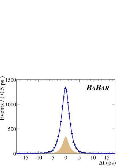
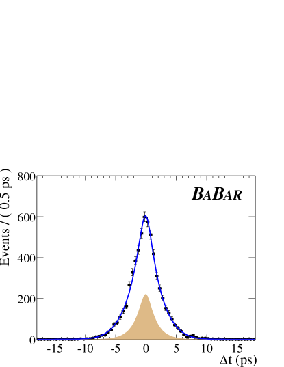
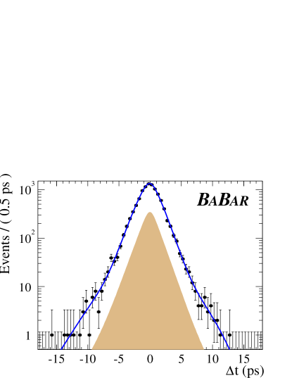
Figure 2: The $\Delta t$ distribution for unmixed and mixed events in the signal sample (opposite-side $D^{*}$-lepton candidates in on-resonance data) and the projection of the fit results. The left-hand plots are for unmixed events; the right-hand plots for mixed events. The shaded area shows the background contribution to the distributions.

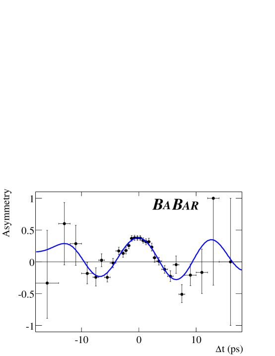
Figure 3: The asymmetry plot for mixed and unmixed events in the signal sample (opposite-side $D^{*}$-lepton candidates in on-resonance data) in the $\delta m$ range from 143 to 148 MeV, and the projection of the fit results. Errors on the data points are computed by considering the binomial probabilities for observing different numbers of mixed and unmixed events while preserving the total number.

Since we float many parameters in the model, it is interesting to see how the errors on $\tau_{B^{0}}$ and $\Delta m_{d}$, and their correlation change when different parameters are free in the fit, or fixed to their best value from the full fit. We perform a series of fits, fixing all parameters at the values obtained from the default fit, except (a) $\Delta m_{d}$  and $\tau_{B^{0}}$, (b) $\Delta m_{d}$, $\tau_{B^{0}}$, and all mistag fractions in the signal model, (c) $\Delta m_{d}$, $\tau_{B^{0}}$, and $f_{B^{+}}$, (d) $\Delta m_{d}$, $\tau_{B^{0}}$, $f_{B^{+}}$, and all mistag fractions in the signal model, (e) all parameters in the signal $\Delta t$ model. The one-sigma error ellipses for these fits and for the default fit are shown in Fig. 4.

We can see that the error on $\tau_{B^{0}}$ changes very little until we float the signal resolution function. Floating the background parameters adds a very small contribution to the error. The contribution from the charged $B$ fraction and mistag fractions to the $\tau_{B^{0}}$ error is negligible. On the other hand, the charged $B$ fraction changes the error on $\Delta m_{d}$ the most. The contributions from floating the mistag fractions, resolution functions, and background $\Delta t$ models are relatively small.

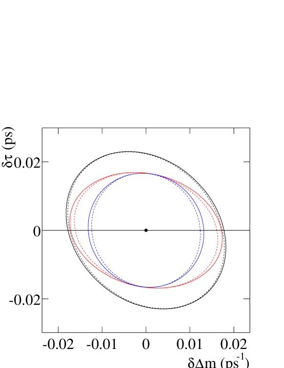
Figure 4: Comparison of one-sigma error ellipses in the $\Delta m_{d}$-$\tau_{B^{0}}$  plane for fits in which different sets of parameters are free. From the innermost to the outermost ellipse, the floating parameters are ($\Delta m_{d}$, $\tau_{B^{0}}$), ($\Delta m_{d}$, $\tau_{B^{0}}$, mistag fractions), ($\Delta m_{d}$, $\tau_{B^{0}}$, $f_{B^{+}}$), ($\Delta m_{d}$, $\tau_{B^{0}}$, $f_{B^{+}}$, mistag fractions), all signal $\Delta t$ parameters, and the default fit (72 floating parameters).

11 Validation and cross checks

In Sec. 11.1, we describe several tests of the fitting procedure that were performed with both fast parameterized Monte Carlo simulations and full detector simulations. In Sec. 11.2, we give the results of performing cross-checks on data, including fitting to different subsamples of the data and fitting with variations to the standard fit.

11.1 Tests of fitting procedure with Monte Carlo simulations

A test of the fitting procedure is performed with fast parameterized Monte Carlo simulations, where 87 experiments are generated with signal and background control sample sizes and compositions corresponding to that obtained from the full likelihood fit to data. The mistag rates and $\Delta t$ distributions are generated according to the model used in the likelihood fit. The full fit is then performed on each of these experiments. We find no statistically significant bias in the average values of $\tau_{B^{0}}$ and $\Delta m_{d}$ for the 87 fits. The RMS spread in the distribution of results is consistent with the mean statistical error from the fits and the statistical error on the results in data, for both $\tau_{B^{0}}$ and $\Delta m_{d}$. We find that 17 of the fits to the 87 experiments result in a value of the negative log likelihood that is smaller (better) than that found in data. We also check the statistical errors on data by measuring the increase in negative log likelihood in data in the two-dimensional ($\tau_{B^{0}}$, $\Delta m_{d}$) space in the vicinity of the minimum of the negative log likelihood. We found that the positive error on $\tau_{B^{0}}$ is about 6% larger than that predicted by the fitting program, whereas the other errors are the same as predicted. We increased the positive statistical error on $\tau_{B^{0}}$ by 6%.

We also fit two types of Monte Carlo samples that include full detector simulation: pure signal and signal plus background. To check whether the selection criteria introduce any bias in the lifetime or mixing frequency, we fit the signal physics model to the true lifetime distribution, using true tagging information, for a large sample of signal Monte Carlo events that pass all selection criteria. We also fit the measured $\Delta t$ distribution, using measured tagging information, with the complete signal $\Delta t$ model described in Sec. 8. We find no statistically significant bias in the values of $\tau_{B^{0}}$ or $\Delta m_{d}$ extracted in these fits.

The $B^{0}\kern 1.79993pt\overline{\kern-1.79993ptB}{}^{0}$, $B^{+}B^{-}$, and $c\overline{c}$ Monte Carlo samples that provide simulated background events along with signal events are much smaller than the pure signal Monte Carlo samples. In addition, they are not much larger than the data samples. In order to increase the statistical sensitivity to any bias introduced when the background samples are added to the fit, we compare the values of $\tau_{B^{0}}$ and $\Delta m_{d}$ from the fit to signal plus background events, and pure signal events from the same sample. We find that when background is added, the value of $\tau_{B^{0}}$ increases by $(0.022\pm 0.009)$ ps and the value of $\Delta m_{d}$ increases by $(0.020\pm 0.005)$ ps^-1, where the error is the difference in quadrature between the statistical errors from the fit with and without background. We correct our final results in data for these biases, which are each roughly the same size as the statistical error on the results in data. We conservatively apply a systematic uncertainty on this bias equal to the full statistical error on the measured result in Monte Carlo simulation with background: $\pm 0.018$ ps for $\tau_{B^{0}}$  and $\pm 0.012$ ps^-1 for $\Delta m_{d}$.

11.2 Cross-checks in data

We perform the full maximum-likelihood fit on different subsets of the data and find no statistically significant difference in the results for different subsets. The fit is performed on datasets divided according to tagging category, $b$-quark flavor of the $D^{*-}\ell^{+}$ candidate, $b$-quark flavor of the tagging $B$, and $D^{0}$ decay mode. We also vary the range of $\Delta t$ over which we perform the fit (maximum value of $|\Delta t|$ equal to 10, 14, and 18 ps), and decrease the maximum allowed value of $\sigma_{\Delta t}$ from 1.8 ps to 1.4 ps. Again, we do not find statisitically significant changes in the values of $\tau_{B^{0}}$ or $\Delta m_{d}$.

12 Systematic studies

We estimate systematic uncertainties on the parameters $\tau_{B^{0}}$ and $\Delta m_{d}$ with studies performed on both data and Monte Carlo samples, and obtain the results summarized in Table 4.

Table 4: Summary of systematic uncertainties on the two physics parameters, $\tau_{B^{0}}$ and $\Delta m_{d}$.

Source	$\delta(\Delta m_{d})$ (ps-1)	$\delta(\tau_{B^{0}})$ (ps)
Selection and fit bias	$0.0123$	$0.0178$
$z$ scale	$0.0020$	$0.0060$
PEP-II boost	$0.0005$	$0.0015$
Beam spot position	$0.0010$	$0.0050$
SVT alignment	$0.0030$	$0.0056$
Background / signal prob.	$0.0029$	$0.0032$
Background $\Delta t$ models	$0.0012$	$0.0063$
Fixed $B^{+}$/$B^{0}$ lifetime ratio	$0.0003$	$0.0019$
Fixed $B^{+}$/$B^{0}$ mistag ratio	$0.0001$	$0.0003$
Fixed signal outlier shape	$0.0010$	$0.0054$
Signal resolution model	$0.0009$	$0.0034$
Total systematic error	$0.013\$	$0.022\$

The largest source of systematic uncertainty on both parameters is the limited statistical precision for determining the bias due to the fit procedure (in particular, the background modeling) with Monte Carlo events. We assign the statistical errors of a full fit to Monte Carlo samples including background to estimate this systematic uncertainty. See Sec. 11.1 for more details.

The calculation of a decay-time difference $\Delta t$ for each event assumes a nominal detector $z$-scale, PEP-II boost, vertical beam-spot position, and SVT internal alignment. We vary each of these assumptions and assign the variation in the fitted parameters as a corresponding systematic uncertainty.

The modeling of the background contributions to the sample determines the probability we assign for each event to be due to signal and the $\Delta t$ distribution we expect for background events. We estimate the systematic uncertainty due to the assumed background $\Delta t$  distributions as the shift in the fitted parameters when we replace the model for the largest background (due to combinatoric events) with a pure lifetime model. We estimate the uncertainty due to the signal probability calculations by repeating the full fit using an ensemble of different signal and background parameters for the $m(D^{*})-m(D^{0})$  distributions, varied randomly according to the measured statistical uncertainties and correlations between the parameters. We assign the spread in each of the resulting fitted physics parameter as the systematic uncertainty.

The model of the charged $B$ background assumes fixed $B^{+}/B^{0}$ ratios for the mistag rates and lifetimes. We vary the mistag ratio by the uncertainty determined from separate fits to hadronic events. We vary the lifetime ratio by the statistical uncertainty on the world average [3]. The resulting change in the fitted physics parameters is assigned as a systematic uncertainty.

The final category of systematic uncertainties is due to assumptions about the resolution model for signal events. We largely avoid assumptions by floating many parameters to describe the resolution simultaneously with the parameters of interest. However, two sources of systematic uncertainty remain: the shape of the outlier contribution, which cannot be determined from data alone, and the assumed parameterization of the resolution for non-outlier events. We study the sensitivity to the outlier shape by repeating the full fit with an ensemble of different shapes, and assign the spread of the resulting fitted values as a systematic uncertainty. We estimate the uncertainty due to the assumed resolution parameterization by repeating the full fit with a triple-Gaussian resolution model and assigning the shift in the fitted values as the uncertainty.

The total systematic uncertainty on $\tau_{B^{0}}$ is 0.022 ps and on $\Delta m_{d}$ is 0.013 ps^-1.

13 Summary

We use a sample of approximately 14,000 exclusively reconstructed $B^{0}\rightarrow D^{*-}\ell^{+}\nu_{\ell}$ signal events to measure the $B^{0}$ lifetime $\tau_{B^{0}}$ and oscillation frequency $\Delta m_{d}$ simultaneously, with an unbinned maximum-likelihood fit. The preliminary results are

$$\tau_{B^{0}}=(1.523^{+0.024}_{-0.023}\pm 0.022)~{}\rm{ps}$$

and

$$\Delta m_{d}=(0.492\pm 0.018\pm 0.013)~{}\rm{ps}^{-1}.$$

The statistical correlation coefficient between $\tau_{B^{0}}$ and $\Delta m_{d}$ is $-0.22$. Both the lifetime and mixing frequency have combined statistical and systematic uncertainties that are comparable to those of the most precise previously-published experimental measurements [3]. The results are consistent with the world average measurements of $\tau_{B^{0}}=(1.542\pm 0.016)~{}\rm{ps}$ and $\Delta m_{d}=(0.489\pm 0.008)~{}\rm{ps}^{-1}$ [3].

14 Acknowledgments

We are grateful for the extraordinary contributions of our PEP-II colleagues in achieving the excellent luminosity and machine conditions that have made this work possible. The success of this project also relies critically on the expertise and dedication of the computing organizations that support BABAR. The collaborating institutions wish to thank SLAC for its support and the kind hospitality extended to them. This work is supported by the US Department of Energy and National Science Foundation, the Natural Sciences and Engineering Research Council (Canada), Institute of High Energy Physics (China), the Commissariat à l’Energie Atomique and Institut National de Physique Nucléaire et de Physique des Particules (France), the Bundesministerium für Bildung und Forschung and Deutsche Forschungsgemeinschaft (Germany), the Istituto Nazionale di Fisica Nucleare (Italy), the Research Council of Norway, the Ministry of Science and Technology of the Russian Federation, and the Particle Physics and Astronomy Research Council (United Kingdom). Individuals have received support from the A. P. Sloan Foundation, the Research Corporation, and the Alexander von Humboldt Foundation.

References

- [1] ARGUS Collaboration, H. Albrecht et al., Phys. Lett. B 192, 245 (1987).
- [2] N. Cabibbo, Phys. Rev. Lett. 10, 531 (1963); M. Kobayashi and K. Maskawa, Prog. Th. Phys. 49, 652 (1973).
- [3] Particle Data Group, K. Hagiwara et al., Phys. Rev. D 66, 010001 (2002).
- [4] The BABAR Collaboration, A. Palano et al., Nucl. Instrum. Methods A 479, 1 (2002).
- [5] “PEP-II: An Asymmetric Factory”, Conceptual Design Report, SLAC-418, LBL-5379 (1993).
- [6] “GEANT, Detector Description and Simulation Tool”, CERN program library long writeup W5013 (1994).
- [7] E687 Collaboration, P. L. Frabetti et al., Phys. Lett. B 331, 217 (1994).
- [8] BABAR Collaboration, B. Aubert et al., “A Study of Time-Dependent -Violating Asymmetries and Flavor Oscillations in Neutral Decays at the ,” SLAC-PUB-9060, hep-ex/0201020, to be published in Phys. Rev. D.