K.-F. Chen
K. Hara
K. Abe
K. Abe
T. Abe
I. Adachi
Byoung Sup Ahn
H. Aihara
M. Akatsu
Y. Asano
T. Aso
V. Aulchenko
T. Aushev
A. M. Bakich
Y. Ban
A. Bay
I. Bedny
P. K. Behera
I. Bizjak
A. Bondar
A. Bozek
M. Bračko
J. Brodzicka
T. E. Browder
B. C. K. Casey
P. Chang
Y. Chao
B. G. Cheon
R. Chistov
S.-K. Choi
Y. Choi
Y. K. Choi
M. Danilov
L. Y. Dong
J. Dragic
S. Eidelman
V. Eiges
Y. Enari
F. Fang
C. Fukunaga
N. Gabyshev
A. Garmash
T. Gershon
B. Golob
A. Gordon
R. Guo
J. Haba
K. Hanagaki
F. Handa
T. Hara
N. C. Hastings
H. Hayashii
M. Hazumi
E. M. Heenan
I. Higuchi
T. Higuchi
L. Hinz
Y. Hoshi
W.-S. Hou
Y. B. Hsiung
S.-C. Hsu
H.-C. Huang
T. Igaki
Y. Igarashi
T. Iijima
K. Inami
A. Ishikawa
R. Itoh
H. Iwasaki
Y. Iwasaki
H. K. Jang
J. H. Kang
J. S. Kang
N. Katayama
H. Kawai
Y. Kawakami
N. Kawamura
H. Kichimi
D. W. Kim
Heejong Kim
H. J. Kim
Hyunwoo Kim
T. H. Kim
K. Kinoshita
S. Korpar
P. Križan
P. Krokovny
R. Kulasiri
S. Kumar
A. Kuzmin
Y.-J. Kwon
J. S. Lange
G. Leder
S. H. Lee
J. Li
R.-S. Lu
J. MacNaughton
G. Majumder
F. Mandl
D. Marlow
T. Matsuishi
S. Matsumoto
T. Matsumoto
K. Miyabayashi
Y. Miyabayashi
H. Miyata
G. R. Moloney
T. Mori
A. Murakami
T. Nagamine
Y. Nagasaka
T. Nakadaira
E. Nakano
M. Nakao
J. W. Nam
Z. Natkaniec
S. Nishida
O. Nitoh
S. Noguchi
S. Ogawa
T. Ohshima
T. Okabe
S. Okuno
S. L. Olsen
Y. Onuki
W. Ostrowicz
H. Ozaki
H. Palka
C. W. Park
H. Park
L. S. Peak
J.-P. Perroud
M. Peters
L. E. Piilonen
N. Root
M. Rozanska
K. Rybicki
H. Sagawa
S. Saitoh
Y. Sakai
H. Sakamoto
M. Satapathy
A. Satpathy
O. Schneider
S. Schrenk
C. Schwanda
S. Semenov
K. Senyo
R. Seuster
M. E. Sevior
H. Shibuya
B. Shwartz
J. B. Singh
N. Soni
S. Stanič
M. Starič
A. Sugi
A. Sugiyama
K. Sumisawa
T. Sumiyoshi
S. Suzuki
S. Y. Suzuki
T. Takahashi
F. Takasaki
N. Tamura
J. Tanaka
M. Tanaka
G. N. Taylor
Y. Teramoto
S. Tokuda
M. Tomoto
T. Tomura
K. Trabelsi
W. Trischuk
T. Tsuboyama
T. Tsukamoto
S. Uehara
K. Ueno
Y. Unno
S. Uno
Y. Ushiroda
G. Varner
K. E. Varvell
C. C. Wang
C. H. Wang
J. G. Wang
M.-Z. Wang
Y. Watanabe
E. Won
B. D. Yabsley
Y. Yamada
A. Yamaguchi
Y. Yamashita
M. Yamauchi
H. Yanai
P. Yeh
M. Yokoyama
Y. Yuan
Y. Yusa
Z. P. Zhang
V. Zhilich
D. Žontar
Aomori University, Aomori, Japan
Budker Institute of Nuclear Physics, Novosibirsk, Russia
Chiba University, Chiba, Japan
Chuo University, Tokyo, Japan
University of Cincinnati, Cincinnati, OH, USA
University of Frankfurt, Frankfurt, Germany
Gyeongsang National University, Chinju, South Korea
University of Hawaii, Honolulu, HI, USA
High Energy Accelerator Research Organization (KEK), Tsukuba, Japan
Hiroshima Institute of Technology, Hiroshima, Japan
Institute of High Energy Physics, Chinese Academy of Sciences, Beijing, PR China
Institute of High Energy Physics, Vienna, Austria
Institute for Theoretical and Experimental Physics, Moscow, Russia
J. Stefan Institute, Ljubljana, Slovenia
Kanagawa University, Yokohama, Japan
Korea University, Seoul, South Korea
Kyoto University, Kyoto, Japan
Kyungpook National University, Taegu, South Korea
Institut de Physique des Hautes Énergies, Université de Lausanne, Lausanne, Switzerland
University of Ljubljana, Ljubljana, Slovenia
University of Maribor, Maribor, Slovenia
University of Melbourne, Victoria, Australia
Nagoya University, Nagoya, Japan
Nara Women’s University, Nara, Japan
National Kaohsiung Normal University, Kaohsiung, Taiwan
National Lien-Ho Institute of Technology, Miao Li, Taiwan
National Taiwan University, Taipei, Taiwan
H. Niewodniczanski Institute of Nuclear Physics, Krakow, Poland
Nihon Dental College, Niigata, Japan
Niigata University, Niigata, Japan
Osaka City University, Osaka, Japan
Osaka University, Osaka, Japan
Panjab University, Chandigarh, India
Peking University, Beijing, PR China
Princeton University, Princeton, NJ, USA
RIKEN BNL Research Center, Brookhaven, NY, USA
Saga University, Saga, Japan
University of Science and Technology of China, Hefei, PR China
Seoul National University, Seoul, South Korea
Sungkyunkwan University, Suwon, South Korea
University of Sydney, Sydney, NSW, Australia
Tata Institute of Fundamental Research, Bombay, India
Toho University, Funabashi, Japan
Tohoku Gakuin University, Tagajo, Japan
Tohoku University, Sendai, Japan
University of Tokyo, Tokyo, Japan
Tokyo Institute of Technology, Tokyo, Japan
Tokyo Metropolitan University, Tokyo, Japan
Tokyo University of Agriculture and Technology, Tokyo, Japan
Toyama National College of Maritime Technology, Toyama, Japan
University of Tsukuba, Tsukuba, Japan
Utkal University, Bhubaneswer, India
Virginia Polytechnic Institute and State University, Blacksburg, VA, USA
Yokkaichi University, Yokkaichi, Japan
Yonsei University, Seoul, South Korea
Abstract
We present measurements of -violating parameters in
and decays based on a 41.8 fb-1 data sample
collected at the resonance with the Belle detector
at the KEKB asymmetric-energy collider. We fully
reconstruct one neutral meson as a eigenstate and identify the flavor of the
accompanying from its decay products. From the distribution of
proper time intervals between pairs of meson decay points, we
obtain the -violating asymmetry parameters ,
and . We also reconstruct
charged decays and determine a
direct- violating asymmetry value of .
††thanks: on leave from National Fermi Accelerator Laboratory, Batavia, IL, USA††thanks: on leave from Nova Gorica Polytechnic, Nova Gorica, Slovenia††thanks: on leave from University of Toronto, Toronto, ON, Canada
In the Kobayashi and Maskawa (KM) model, violation is
incorporated as an irreducible complex phase in the
weak-interaction quark mixing matrix [1]. Measurements of
sin, where arg, from
violation in decays by the
Belle [2] and BaBar [3]
collaborations established violation in the neutral meson
system that is consistent with KM expectations. Measurements of
sin based on other decay modes, especially charmless
modes that are mediated by diagrams that contain virtual particle
loops, provide important tests of the KM model. In this letter we
describe the first measurement of -violating asymmetries in
the penguin-mediated decay , and an
improved measurement of the direct -violating asymmetry in the
decay [4].
The KM model predicts -violating asymmetries in the
time-dependent rates for and decay to a
common eigenstate, . When an decays
into a meson pair, the two mesons remain in
a coherent -wave state until one of them decays. The decay of
one of the mesons at time to a final state,
, which distinguishes between and
, projects the accompanying meson onto the
opposite -flavor which decays to at time
. The decay rate has a time dependence given by
(1)
where is the time-dependent
asymmetry, is the lifetime, , and the -flavor when the
accompanying meson is a ().
Within the framework of the Standard Model (SM), the charmless
decay proceeds primarily via
penguin diagrams; there is a small contribution from a
color-suppressed tree diagram, but that amplitude is
expected to be only a few percent of that for the
penguin [5, 6, 7]. Thus,
violation in this decay mode, to a good approximation, measures
, and one can compare the result to the value measured for
. Phases from new physics in the
penguin loop could show up as a difference between the two
measured values [5, 8]. Since the branching
fraction of appears to be anomalously large
[9, 10, 11], this mode is
especially interesting to search for effects of an additional
phase besides due to physics beyond the
SM [5].
The time-dependent asymmetry can be expressed as
(2)
where the -violating parameters and are given by
(3)
in which is a complex parameter that
depends on both - mixing and the decay
amplitude for . The
SM value for is very nearly equal to the absolute
value of the ratio of the to decay
amplitudes. Therefore , or equivalently
, indicates direct
violation. The direct asymmetry, , in charged decays can also
be investigated from the time-integrated decay rates of
versus . To a good approximation the -violating
parameter, , in the decay is equal to the parameter ,
which can be directly compared with the value measured from decays.
The measurement reported here is based on a 41.8 fb-1 data
sample, which contains 44.8 million pairs,
collected with the Belle detector at the KEKB asymmetric energy
(3.5 GeV on 8 GeV) collider [12] operating at the
resonance. At KEKB, the is produced
with a Lorentz boost of nearly along the
electron beam direction (). Since the and
mesons are approximately at rest in the
center-of-mass system, can be determined
from the displacement in between the and
decay vertices: .
The Belle detector is a large solid-angle general purpose magnetic
spectrometer that consists of a three-concentric-layer silicon
vertex detector (SVD), a 50-layer central drift chamber (CDC), an
array of aerogel threshold Čerenkov counters (ACC),
time-of-flight scintillation counters (TOF), and an
electromagnetic calorimeter comprised of 8736 CsI(Tl) crystals
(ECL) located inside a superconducting solenoid coil that
provides a 1.5 T magnetic field. An iron flux-return located
outside of the coil is instrumented to detect muons and mesons
(KLM). The detector is described in detail
elsewhere [13].
The event selection closely follows the
method described in detail in a previously published report that
describes the branching ratio measurement [11];
the time-dependent analysis is similar to that used for and presented in Ref. [14].
For the analysis reported here, the event selection is slightly
modified for the time-dependent measurement from what described in
Ref. [11] in order to retain more signal events
and to keep better control of systematic errors. Candidate decays are reconstructed from pairs of oppositely
charged tracks that are constrained to a common vertex and have an
invariant mass that is within MeV/ of the nominal
mass. Two decay channels are used for
reconstruction:
() with
(); and
() with . To
increase the event yield, we omit the minimum transverse momentum
requirement for charged tracks that was used in
Ref. [11]. Instead, we require that all of the
tracks have associated SVD hits and radial impact parameters cm projected on the - plane. Better tracking
requirement improves the vertex determination and gives less bias
due to detector asymmetry. Particle identification information
from the ACC, TOF and CDC measurements are used to form a
likelihood ratio in order to distinguish pions from kaons with at
least 2.5 separation for laboratory momenta up to 3.5
GeV/. Candidate photons from
decays are
required to be isolated and have MeV from
the ECL measurement. The invariant mass of
candidates is required to be between 500 MeV/ and
570 MeV/. A kinematic fit with an mass constraint is
performed using the fitted vertex of the tracks from
the as the decay point. For
decays, the candidate mesons
are reconstructed from pairs of vertex-constrained
tracks with an invariant mass between 550 and 920 MeV/. The
candidates are required to have a reconstructed mass
from 940 to 970 MeV/ for the mode
and 935 to 975 MeV/ for mode.
Charged candidates are selected for the decay based on the particle identification
information described in Ref. [11].
Candidate mesons are identified by combining and
() candidates to form the beam-constrained mass
, and the energy difference , where
is the center of mass (cms) beam energy (nominally GeV),
and and are the cms energy and
momentum of the candidate. The signal region is
defined as GeV/; the signal
region depends on the mode: it is GeV
GeV for and
GeV for .
We extract the signal yields with a simultaneous unbinned
maximum-likelihood (ML) fit for both and .
The signal distribution
is a product of a Gaussian function in and a Gaussian
plus a bifurcated Gaussian tail function in . The means
and widths, as well as an overall normalization are the fitting
parameters. The shapes of the background distributions, described
below, are determined from sideband events in the GeV/
GeV/ and GeV
region, but with GeV or GeV for
the mode and GeV for the mode;
the difference is due to slight differences in resolution in the
data as well as in the Monte Carlo simulation determined from the
higher statistics mode.
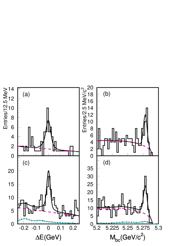
Figure 1: The and distributions for the
candidates (histogram) and the ML fit results
(solid curve); (a) and (b) show the
mode, (c) and (d) the mode. The dashed
curves are the results of the fit for continuum
background; the dash-dot curves in (c) and (d) show the expected
background in the mode from the Monte
Carlo simulation.
The dominant backgrounds are from
continuum events (). In this case, signal and
background events can be partially separated by the event
topology, which tends to be jet-like for continuum
events and nearly isotropic for events. We use
, the cosine of the angle between the thrust
axis of the candidate and that of the other particles in cms.
The requirement rejects of the
background while retaining of the signal events. This is
sufficient for the mode, which is
relatively clean.
For the channel, an additional cut is
applied using event shape variables. These variables include
, which is the scalar sum of the transverse momenta of
all particles outside a cone around the candidate
direction divided by the scalar sum of their total
momenta, and five modified Fox-Wolfram moments [15], all
combined into a single Fisher discriminant. In addition, we use
, the cosine of the angle between the
candidate flight direction and the beam axis () in the cms, and
a helicity variable , which is the cosine of the angle
between the momentum direction in the rest frame
and the momentum direction in the rest frame.
All of these variables are combined to form a likelihood ratio , where is
the product of signal () probability density
functions. We determine from Monte Carlo (MC) and
from sideband data. We require for
the mode, which rejects of the
background and retains of the signal.
Sideband events are used to determine the shape of the continuum
background distributions for the mode
and modes separately. The
shape is modelled by a linear background obtained from the sideband. The shape is modelled by the empirical
function of Ref. [16]. From the ML fit we determine
the total background fraction in the signal region to be
for the mode and 56.5% for the
mode. The backgrounds are
predominantly continuum events with small
contributions from other generic decays, mainly
due to charm daughter particles from or decay.
These backgrounds, which are determined from a sample of MC
simulated generic meson decays, are negligible for the
mode (smaller than ), but
contribute of the total background for the
mode. The larger background for
the mode is due to wide width of
mass and combinatorial background of and to
form candidates.
In the case of multiple candidates from the same event, we select
the candidate with the best value from the
mass constrained fit. The signal efficiency is determined from MC
events to be for
(). From the above-described ML
fit, we obtain signal events in the
mode and
events in the mode; the results of
the fits are shown in Fig. 1.
Leptons, baryons, and charged pions and kaons that are
not associated with the reconstructed
decay are used to identify the flavor of the accompanying
meson. We apply the same method used for the Belle
measurement [2]. We use two parameters, and
, to represent the tagging information: is a discrete
variable that corresponds to the sign of the quark charge and
has the value for a (i.e., ) tag, and
for a () tag; is an
event-by-event, MC-determined flavor-tagging dilution factor that
ranges from (no flavor discrimination) to (unambiguous
flavor assignment). The value of is used to sort data into six
intervals of , according to flavor purity, the corresponding
wrong tag fractions, , and dilution factors
() are determined for each bin from data as described
in Ref. [2].
The vertex positions for the and
decays are reconstructed using tracks that have at least one
three-dimensional space point determined from associated
- and hits in the same SVD layer and one or more
additional hits in the other layers. Each vertex position is
required to be consistent with the interaction point profile
smeared in the - plane by the average transverse
meson decay length. The vertex is determined from
all remaining well reconstructed tracks after the candidate tracks are removed. Tracks from other
candidates are not used. The MC simulation indicates that
the typical combined track-finding and vertex-finding efficiency
is 83 for decays and 95 for the
decays. The typical vertex resolution (rms) is
147m (89m) for the
() mode on the side, and 159m
for the on the tagging side.
The proper-time interval resolution for the signal, , is obtained by convolving a sum of two Gaussians
(a main component due to the SVD vertex resolution and
charmed meson lifetimes, plus a tail component to account
for poorly reconstructed tracks) with a function that takes into
account the cms motion of the mesons. The fraction in the main
Gaussian is determined to be from a study of
control samples of fully reconstructed
mesons [2]. The means (,
) and widths (, ) of the Gaussians are calculated event-by-event from the
and vertex fit error matrices
and the values from the fits [17].
The background resolution has the
same functional form but the parameters are obtained also
event-by-event from the and sideband
events. We obtain the lifetimes for neutral and charged mesons
for the channels using the same procedure; the
results [18] are consistent with the world
average values.
After vertexing, we find 77 candidate events with ()
flavor tags and 74 candidate events with
() for .
Figures 2(a) and 2(b)
show the observed distribution for the two samples.
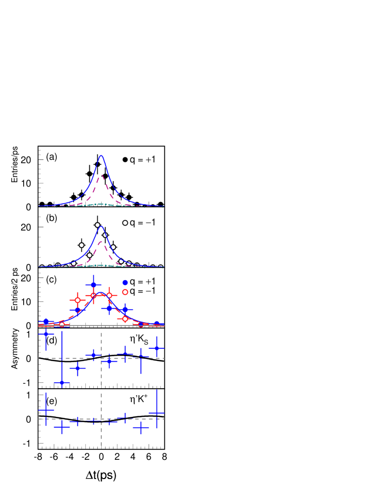
Figure 2: The distributions for the candidates in the signal region: (a) candidates with
, i.e. the tag side is identified as ; (b) candidates
with ; (c) yields after background
subtraction; (d) the asymmetry for after background subtraction; (e) the same asymmetry
calculated for events. The curves in the
figures show the results of the unbinned maximum likelihood fit.
In (a) and (b), the solid, dashed and dash-dot curves are fit
results for the total, background and
background respectively. In (c) the solid (dashed)
curve is for the () signal fit. In (d) and (e), the
solid curve is the fit result for and while the dashed
curve corresponds to zero asymmetry.
We determine the -violating parameters, and , by
performing an unbinned ML fit to the observed
distributions. For perfect resolution, the probability density
function (pdf) for the signal, , as a
function of and is given by Eqs. 1 and
2 with replaced by to take into
account the dilution due to mis-tagging. We fix and
at their world average values [19]. The pdf
used for the background distribution is
(4)
where is the background fraction with an
effective lifetime and is the Dirac
delta function. We determine and
ps from the sideband data. The pdf used to
account for the small generic background for the
mode is . This
background is mainly due to mis-reconstructed secondary (charm)
decays, such as , ,
and , etc. with mesons
decaying into a kaon and multiple pions or a meson.
We define the likelihood value for each event as:
(5)
Here ( or
and ) are the weighted probability functions determined
on an event-by-event basis as a function of and , properly normalized by the average signal and background
fractions in the fitting region for each interval for the
signal , and
events, defined as
(6)
Here and are the shape functions for
the signal (), continuum background () and
background ().
The average event fractions, , are measured for
and separately in each interval.
In the fit, and are free parameters that are determined by
maximizing the likelihood function ,
where the product is over all
candidates. After maximizing the combined likelihood, the
asymmetry parameters are determined from a total of 72.9
signal events (37.3 - and 35.6
-tags) to be:
,
.
Figures 2(a) and (b) show the
distribution for - and -tagged events
together with the fit curves; the background-subtracted
distributions for signal-only are shown in
Fig. 2(c). The errors on data points in
Fig. 2(c) are statistical only and do not
include the error associated with the subtracted background
obtained by the fit. The background-subtracted time-dependent
asymmetry between the - and -tagged events
is shown as a function of in
Fig. 2(d), with the result of the fit for
and superimposed.
The systematic errors are summarized in Table 1
for and . The dominant sources for are due to uncertainties in the signal and
background determination ( and pdf’s, event
fractions and background shape), resolution functions, wrong tag
fractions, vertexing, and the physics parameters ( and
). For , the
uncertainties in the signal and background determination and the
vertexing are the leading components. We determine the systematic
error due to physics parameters by repeating the fit after varying
those parameters within their error taken from the world
average [19]. The systematic errors for wrong tag fractions,
resolution functions, signal and background pdf’s are estimated by
repeating the fit after varying the parameters by
determined from the data or MC. The systematic error due to
vertexing is studied by varying the cut on vertex or
removing it and then repeat the fit.
A number of checks are also performed. We analyze the
sample in the same way as .
The raw asymmetry for the candidates
is shown in Fig. 2(e). A fit to 230
candidate events yields and
, consistent with no asymmetry, as
expected. We also examine the event yields and the
distributions for - and -tagged events in
the and sideband region. We find no
significant difference between the two samples in both the
and modes. The average raw
asymmetry from the sideband data is , which is
consistent with zero and indicates no bias.
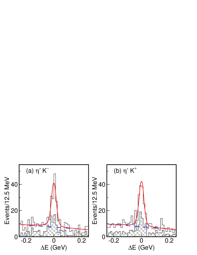
Figure 3: The projection plots for the
candidates: (a) for , (b) for . The
cross hatched histograms indicate the channel; the solid
histograms are the sum of both decay channels
( and ). The curves are the fitted backgrounds
(dashed) and the sum of signal and background (solid).
We also analyze the self-tagged event sample
to search for a direct asymmetry. Here we do not use
flavor-tag information from the other meson. The sample is divided into and samples. Since the asymmetry () for
is time independent, we use the same event selection and analysis
procedure as described in Ref. [11]. A
simultaneous ML fit to and is performed
for each sub-sample. The fitted numbers of signal events in the
() mode are
() for decays
and () for
decays, respectively. The number of produced and
events are obtained by maximizing the product of the likelihoods
for each submode, as shown in Fig. 3. From the
fit we obtain
for the mode and for
; here the errors are statistical only.
Since the systematic errors on reconstruction and
the number of events cancel in the ratio, the
systematic uncertainty in comes
mainly from the reconstruction efficiency of charged kaons and the
ML fit. The asymmetry in the efficiency is studied using
inclusive charged kaons in the same kinematic range as the signal.
The uncertainty due to fitting is measured by varying the
parameters of the fit functions. We find the systematic errors in
are from
reconstruction and from the ML fit. The combined
for the decay is determined to be
,
which is consistent with zero. Combining the errors in quadrature
and assuming a Gaussian distribution, we find the
confidence level interval is , which is a factor of two more restrictive than our
previous measurement [11].
In summary, we have measured the asymmetry parameters in
and decays based on a 41.8 fb-1 data sample
collected with the Belle detector. The result for
decay-time-integrated direct asymmetry, , is
small and consistent with zero. Our results for the
time-dependent asymmetry parameters and are the first
measurements of asymmetry parameters related to with
a charmless decay mode. In the SM, to a good approximation
the value of should be equal to
measured in decays, where
the current world average is [20].
With a much larger data sample, we will significantly reduce the
uncertainty in and impose tight
constraints on phases from new physics beyond the Standard Model.
We wish to thank the KEKB accelerator group for the excellent
operation of the KEKB accelerator. We acknowledge support from the
Ministry of Education, Culture, Sports, Science, and Technology of
Japan and the Japan Society for the Promotion of Science; the
Australian Research Council and the Australian Department of
Industry, Science and Resources; the National Science Foundation
of China under contract No. 10175071; the Department of Science
and Technology of India; the BK21 program of the Ministry of
Education of Korea and the CHEP SRC program of the Korea Science
and Engineering Foundation; the Polish State Committee for
Scientific Research under contract No. 2P03B 17017; the Ministry
of Science and Technology of the Russian Federation; the Ministry
of Education, Science and Sport of the Republic of Slovenia; the
National Science Council and the Ministry of Education of Taiwan;
and the U.S. Department of Energy.
References
[1]
M. Kobayashi and T. Maskawa,
Prog. Theor. Phys. 49 (1973) 652.
[2]
Belle Collaboration, K. Abe et al.,
Phys. Rev. Lett. 87 (2001) 091802;
A. Abashian et al.,
Phys. Rev. Lett. 86 (2001) 2509; and
K. Abe et al., hep-ex/0202027, to be published in Phys. Rev. D.
[3]
BaBar Collaboration, B. Aubert et al.,
Phys. Rev. Lett. 87 (2001) 091801;
B. Aubert et al.,
Phys. Rev. Lett. 86 (2001) 2515; and
B. Aubert et al., hep-ex/0201020, to be published in Phys.
Rev. D.
[4]
Charge conjugate modes are implicitly included throughout the
paper unless explicitly stated.
[5]
D. London and A. Soni,
Phys. Lett. B 407 (1997) 61.
[6]
A. Ali, G. Kramer and C.-D. Lu,
Phys. Rev. D 59 (1999) 014005.
[7]
E. Kou and A. I. Sanda,
Phys. Lett. B 525 (2002) 240.
[8]
T. Moroi,
Phys. Lett. B 493 (2000) 366.
[9]
CLEO Collaboration, S. J. Richichi et al.,
Phys. Rev. Lett. 85 (2000) 520.
[10]
BaBar Collaboration, B. Aubert et al.,
Phys. Rev. Lett. 87 (2001) 221802.
[11]
Belle Collaboration, K. Abe et al.,
Phys. Lett. B 517 (2001) 309.
[12]
E. Kikutani ed., KEK Preprint 2001-157 (2001), to appear in
Nucl. Inst. and Meth. A.
[13]
Belle Collaboration, A. Abashian et al.,
Nucl. Inst. and Meth. A 479 (2002) 117.
[14]
Belle Collaboration, K. Abe et al.,
KEK Preprint 2002-6 and hep-ex/0204002,
submitted to Phys. Rev. Lett.
[15]
The Fox-Wolfram moments were introduced in G. C. Fox, S. Wolfram,
Phys. Rev. Lett. 41 (1978) 1581.
The Fisher discriminant used by Belle in this analysis is
described in [11].
[16]The functional form is
, where .
H. Albrecht et al. (ARGUS Collaboration),
Phys. Lett. B 241 (1990) 278; 254 (1991) 288.
[17]
Typical values are ps, ps
and ps, ps.
[18]We obtain
ps for the
mode (the world average [19] is ps) and
ps for the
mode (the world average is ps).
[19]
Particle Data Group, D. E. Groom et al.,
Eur. Phys. J. C 15 (2000) 1.
[20]This average includes recent updated results from
Belle: T. Higuchi, hep-ex/0205020; and BaBar: B. Aubert et al., hep-ex/0203007.
![[Uncaptioned image]](/html/hep-ex/0207033/assets/x1.png)