Measurement of the $D^{+}$ and $D_{s}^{+}$ decays into $K^{+}K^{-}K^{+}$.

Abstract

We present the first clear observation of the doubly Cabibbo suppressed decay $D^{+}\rightarrow K^{-}K^{+}K^{+}$ and the first observation of the singly Cabibbo suppressed decay $D_{s}^{+}\rightarrow K^{-}K^{+}K^{+}$. These signals have been obtained by analyzing the high statistics sample of photoproduced charm particles of the FOCUS (E831) experiment at Fermilab. We measure the following relative branching ratios:

$\Gamma\left(D^{+}\rightarrow K^{-}K^{+}K^{+}\right)/\Gamma\left(D^{+}\rightarrow K^{-}\pi^{+}\pi^{+}\right)=(9.49\pm 2.17\pm 0.22)\times 10^{-4}$

and

$\Gamma\left(D_{s}^{+}\rightarrow K^{-}K^{+}K^{+}\right)/\Gamma\left(D_{s}^{+}\rightarrow K^{-}K^{+}\pi^{+}\right)=(8.95\pm 2.12~{}^{+2.24}_{-2.31})\times 10^{-3}$,
where the first error is statistical and the second is systematic.

$\textrm{The~{}FOCUS~{}Collaboration}^{\star}$

1 Introduction

Doubly Cabibbo suppressed (DCS) charm decays are expected to occur with a rate which is roughly a factor $\tan^{4}\theta_{C}\sim 2.5\times 10^{-3}$ smaller than the corresponding Cabibbo favored (CF) modes. This is the main reason our present knowledge of these decays is rather poor and limited to very few decay modes. Only four DCS decays have been observed, $D^{+}\rightarrow K^{+}\pi^{-}\pi^{+}$, $D^{0}\rightarrow K^{+}\pi^{-}$, $K^{+}\pi^{-}\pi^{0}$ and $K^{+}\pi^{-}\pi^{+}\pi^{-}$. The interpretation of the $D^{0}$ modes is complicated by possible contributions from $D^{0}-\overline{D^{0}}$ mixing [4, 5, 6, 7], making the $D^{+}\rightarrow K^{+}\pi^{-}\pi^{+}$ decay the only pure DCS decay previously studied.

In this paper, we report the first clear observation of the DCS decay $D^{+}\rightarrow K^{-}K^{+}K^{+}$, together with the first observation of the singly Cabibbo suppressed (SCS) decay of $D_{s}^{+}$ into the same final state. Throughout this paper, the charge conjugate is implied when a decay mode of a specific charge is stated.

It is interesting to note that in contrast to the four modes previously mentioned, the DCS decay $D^{+}\rightarrow K^{-}K^{+}K^{+}$ cannot result from a simple spectator process, but presumably requires the intervention of strong resonances that simultaneously couple to the $\pi\pi$ and $KK$ channels. It could also proceed through annihilation but from studies of $D_{s}^{+}\rightarrow\pi^{-}\pi^{+}\pi^{+}$ we expect this contribution to be small [8].

The results presented in this paper have been obtained using the high statistics charm sample of the FOCUS experiment at Fermilab. FOCUS is a charm photoproduction experiment which took data during the 1996/1997 fixed target run at Fermilab. The FOCUS detector is a large aperture, fixed-target spectrometer with excellent vertexing and particle identification. A photon beam is derived from the bremsstrahlung of secondary electrons and positrons with an $\approx 300$ GeV endpoint energy produced from the 800 GeV/$c$ Tevatron proton beam. The photon beam interacts in a segmented BeO target. The charged particles which emerge from the target are tracked by two systems of silicon microvertex detectors. The upstream system, consisting of 4 planes (two views in 2 stations), is interleaved with the experimental target, while the other system lies downstream of the target and consists of twelve planes of microstrips arranged in three views. These detectors provide high resolution separation of primary (production) and secondary (decay) vertices with an average proper time resolution of $\approx 30$ fs for 2-track vertices. The momentum of a charged particle is determined by measuring its deflections in two analysis magnets of opposite polarity with five stations of multiwire proportional chambers. Three multicell threshold Čerenkov counters are used to discriminate between electrons, pions, kaons, and protons.

2 Signals and selection criteria

The final states are selected using a candidate driven vertex algorithm. The basic idea of this algorithm is to use a charm candidate decay vertex as a seed to find the primary vertex. In our particular case a decay vertex is formed from three reconstructed charged tracks and the momentum vector of the resultant D candidate is used to intersect other reconstructed tracks and search for a suitable production vertex. The confidence levels of both vertices are required to be greater than $1\%$. We measure $\ell$ the separation of the two vertices and its associated error $\sigma_{\ell}$. The quantity $\ell/\sigma_{\ell}$ is the significance of detachment of the secondary and primary vertices. Cuts on $\ell/\sigma_{\ell}$ are used to extract the $D$ signals from non-charm background and to improve the signal to background ratio. Two other measures of vertex isolation are used: a primary vertex isolation and a secondary vertex isolation. The primary vertex isolation cut requires that the confidence level for one of the tracks assigned to the decay vertex to be included in the primary vertex be less than a certain threshold value. The secondary vertex isolation cut requires that the maximum confidence level for all tracks not assigned to any vertex to form a vertex with the $D$ candidate be less than a certain threshold value. The main difference in the selection criteria between different decay modes lies in the particle identification cuts applied to the decay products. To minimize the systematic errors we use identical vertex cuts both on the signal and normalizing modes.

In the $D^{+}\rightarrow K^{-}K^{+}K^{+}$ analysis we require $\ell/\sigma_{\ell}>8$. The primary and secondary vertex isolation must be less than $0.1\%$. The $D$ momentum must be in the range $25~{}\textrm{GeV}/c$ to $250~{}\textrm{GeV}/c$ and the primary vertex must be formed with at least two reconstructed tracks in addition to the seed track. We require that the decay vertex occur outside of the target material. For each charged track the Čerenkov algorithm computes four likelihoods from the observed firing response of all the cells that lie inside the track’s Čerenkov cone for every counter [9]. The product of all firing probabilities for all cells within the three Čerenkov cones produces a $\chi^{2}$-like variable $W_{i}=-2\ln(\mathrm{Likelihood})$, where $i$ ranges over electron, pion, kaon and proton hypotheses. We require observed Čerenkov light pattern for the kaon hypothesis is favored over that for the pion hypothesis by more than a factor of exp(0.5) by requiring $W_{\pi}-W_{K}>1.0$. We also apply a kaon consistency cut, which requires that no particle hypothesis is favored over the kaon hypothesis with a $\Delta W=W_{K}-W_{\textrm{min}}$ exceeding $3.5$. To further reduce the background due to poorly reconstructed candidates, we require that the proper time resolution of the candidates, defined as $\sigma_{\ell}/(\beta\gamma c)$, be less than $150$ fs.

The resulting $D^{+}$ signal is shown in Fig.1(a). We obtain a Gaussian yield of $65.5\pm 15.0$ $D^{+}\rightarrow K^{-}K^{+}K^{+}$ events over a linear background. The mass value returned by the fit is $1869\pm 1~{}\textrm{MeV}/c^{2}$; the r.m.s. of the Gaussian fit is $5.2\pm 1.2~{}\textrm{MeV}/c^{2}$ in agreement with Monte Carlo simulations. The two broad structures around $1985~{}\textrm{MeV}/c^{2}$ and $2085~{}\textrm{MeV}/c^{2}$ are due to $D^{+}$ and $D_{s}^{+}$ decays into $K^{-}K^{+}\pi^{+}$ where the $\pi^{+}$ is misidentified as a $K^{+}$.

In the $D_{s}^{+}\rightarrow K^{-}K^{+}K^{+}$ analysis we have to use stronger Čerenkov cuts to extract the signal which otherwise would be completely hidden by the $K^{-}K^{+}\pi^{+}$ mis-identification peaks. We require $W_{\pi}-W_{K}>4.5$ for all three kaon candidates. All the other cuts are the same as for the $D^{+}\rightarrow K^{-}K^{+}K^{+}$ decay.

Fig.1(b) shows the invariant mass plot where both $D^{+}$ and $D_{s}^{+}$ peaks are now evident. In the fit the $D_{s}^{+}$ mass and width are fixed to the values found in the Monte Carlo. This is done to reduce the effects of any residual fluctuation of the $D^{+}\rightarrow K^{-}K^{+}\pi^{+}$ reflection, which would induce a shift of the peak toward higher masses. We obtain a yield of $31.4\pm 7.4$ $D_{s}^{+}\rightarrow K^{-}K^{+}K^{+}$ events over a linear background.

For $D^{+}\rightarrow K^{-}K^{+}K^{+}$ we measure the branching ratio relative to $D^{+}\to K^{-}\pi^{+}\pi^{+}$, while for $D_{s}^{+}\rightarrow K^{-}K^{+}K^{+}$ that relative to $D_{s}^{+}\to K^{-}K^{+}\pi^{+}$. We obtain:

$\Gamma\left(D^{+}\rightarrow K^{-}K^{+}K^{+}\right)/\Gamma\left(D^{+}\rightarrow K^{-}\pi^{+}\pi^{+}\right)=(9.49\pm 2.17)\times 10^{-4}$

$\Gamma\left(D^{+}_{s}\rightarrow K^{-}K^{+}K^{+}\right)/\Gamma\left(D^{+}_{s}\rightarrow K^{+}K^{-}\pi^{+}\right)=(8.95\pm 2.12)\times 10^{-3}$.

The cuts on the normalization modes are identical whenever possible to those used for the selection of the corresponding $3K$ signal. In addition, to remove contamination from the $D_{s}^{+}\to K^{-}K^{+}\pi^{+}$ normalization mode due to Čerenkov misidentified $D^{+}\to K^{-}\pi^{+}\pi^{+}$ events, we employ an anti-reflection cut to reject candidates which, when reconstructed as $K^{-}\pi^{+}\pi^{+}$, lie within $2$ sigma of the $D^{+}$ nominal mass. The normalization signals are shown in Fig.1(c) and Fig.1(d) and consist of $62911\pm 263$ and $3844\pm 66$ events respectively.

In all our simulations we always used the proper resonant substructure for the two normalization modes [10] [11], which would otherwise produce important systematic deviations of the results.

Figure 1: Invariant mass distributions for $D^{+}\to K^{-}K^{+}K^{+}$(a), $D_{s}^{+}\to K^{-}K^{+}K^{+}$(b), $D^{+}\to K^{-}\pi^{+}\pi^{+}$(c) and $D_{s}^{+}\to K^{-}K^{+}\pi^{+}$(d).

3 Systematic Errors

We performed a detailed investigation of any source of systematics which could impact our branching ratio measurements. We first studied the stability of the results by varying the cuts over a wide range of values. Our results are stable in their evolution on the most critical cuts: $\ell/\sigma_{\ell}$, $W_{\pi}-W_{K}$ and primary and secondary vertex isolation.

We then split the samples using variables which can probe different kinematical regions, such as low and high momentum range, or different experimental conditions, such as early and late runs, which have different target configurations. In doing this we can check our results together with our Monte Carlo simulation over a variety of different conditions. We quantify a “split sample systematic error” by examining consistency among these statistically independent splits of our data. If the consistency $\chi^{2}$ turns out to be smaller than $1$, this error is taken to be zero. Otherwise we scale all the errors up to bring the $\chi^{2}$ back to $1$. The split sample systematic error is then defined as the difference in quadrature between the scaled error of the weighted average of the subsample estimates and the statistical error of the total data set. This procedure is similar to the $S$-factor method used by the Particle Data Group [14].

We have split our sample by high and low $D$-momentum, $D$ and $\bar{D}$, and early and late run periods. Splits have been done in one variable at a time because of our limited statistics.

The measured branching ratios for the three pairs of disjoint samples are shown in Fig.2. We find only one contribution to the systematic uncertainty, namely the run-period split sample for the $D_{s}^{+}$ decay which gives a contribution to the branching ratio systematics of 2.23$\times$10^-3.

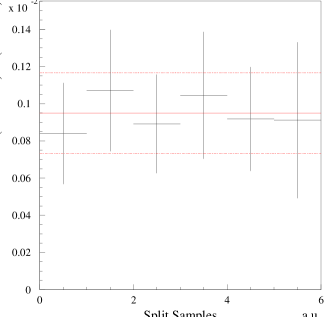
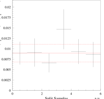
Figure 2: Split sample results for $D$(a) and $D_{s}$(b) relative branching ratios. Three pairs of disjoint samples are considered: high and low momenta on the left, late and early runs in the center, $D$ and $\bar{D}$ on the right. The lines show the joint sample and the $1\sigma$ error bars.

In computing the branching ratios we have used the efficiency of a pure phase-space decay. This choice was motivated by the relatively flat distribution of the events over the Dalitz domains as shown in Fig. 3.

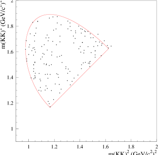
Figure 3: Dalitz plot for $D^{+}$(a) and for $D_{s}^{+}$(b). Only events which lie within $2\sigma$ of the respective nominal masses are plotted.

To better investigate the implications of this assumption we have computed the reconstruction efficiencies for two particularly representative cases, a $\phi K^{+}$ decay and a $f_{0}(980)K^{+}$ decay. Table 1 shows the calculated efficiencies with respect to those for pure phase-space decays.

	$\epsilon(D^{+})$	$\epsilon(D_{s}^{+})$
Phase-Space	$1$	$1$
$\phi K^{+}$	$0.927\pm 0.015$	$0.948\pm 0.015$
$f_{0}(980)K^{+}$	$1.028\pm 0.014$	$1.086\pm 0.014$

Table 1: Reconstruction efficiencies, $\epsilon$, for different decay dynamics into the same $K^{-}K^{+}K^{+}$ final state for $D^{+}$ and $D_{s}^{+}$.

Given the non-negligible variation of the efficiency values, we considered the following two cases in order to assess the systematic uncertainty: the decay proceeds through the maximum estimated amount of $\phi K^{+}$ component, the remaining being pure phase space; the decay proceeds through the maximum estimated amount of $f_{0}(980)K^{+}$ component, the remaining being pure phase space. The estimated fractions, shown in Table 2, have been obtained by fits to the $3K$ invariant mass plots requiring that the $K^{+}K^{-}$ invariant mass lie within $2\sigma$ of the nominal $\phi$ mass for the $\phi K^{+}$ decay and between two kaon mass threshold and $1.05~{}\textrm{GeV/}c^{2}$ for the $f_{0}(980)K^{+}$ decay. These estimates are crude and represent conservative upper limits for the purpose of estimating systematic errors and are not meant to be measurements.

	$D^{+}$	$D_{s}^{+}$
$\phi K^{+}$	$12.4\%$	$18.75\%$
$f_{0}(980)K^{+}$	$44.5\%$	$72\%$

Table 2: Estimated fraction of $\phi K^{+}$ and $f_{0}(980)K^{+}$ components for $D^{+}$ and $D_{s}^{+}$ decays.

Under these assumptions, the contribution to the total systematics on the branching ratio measurement is $\pm 0.10\times 10^{-4}$ for $D^{+}$ and ${}^{+0.09}_{-0.52}\times 10^{-3}$ for $D_{s}^{+}$.

The last source of systematic error we studied is that due to fitting procedure. We calculated our branching ratios for various fit conditions, such as changing the parametrization of the background shapes, rebinning the histograms, including in the $D^{+}$ fit the $K^{-}K^{+}\pi^{+}$ reflection peaks and varying the fixed $D_{s}^{+}$ mass value by $1\sigma$ of the quoted error [14]. Since all these results are a priori likely we used the resulting sample variance to estimate the associated systematics. We obtain a systematic contribution of $\pm$0.19$\times$10^-4 for the $D^{+}$ decay mode and ${}^{+0.12}_{-0.33}\times 10^{-3}$ for the $D_{s}^{+}$.

In conclusion, summing in quadrature the different systematic errors we obtain our final results:

$BR\left(D^{+}\rightarrow K^{-}K^{+}K^{+}\right)/\left(D^{+}\rightarrow K^{-}\pi^{+}\pi^{+}\right)=(9.49\pm 2.17\pm 0.22)\times 10^{-4}$

and

$BR\left(D^{+}_{s}\rightarrow K^{-}K^{+}K^{+}\right)/\left(D^{+}_{s}\rightarrow K^{-}K^{+}\pi^{+}\right)=(8.95\pm 2.12~{}^{+2.24}_{-2.31})\times 10^{-3}$

4 Conclusions

Our $D^{+}$ measurement is consistent with the E687 upper limit [3] and constitutes the first clear evidence for this DCS decay. Our data indicate that only a minor fraction, if any, of the decay proceeds through the $\phi K^{+}$ channel. This could suggest that the decay proceeds mainly through resonances that can couple to both $\pi\pi$ and $KK$, such as the $f_{0}$ resonance series, as expected from a naive spectator picture. However, more statistics would be needed to make quantitative statements through a Dalitz analysis.

Our $D_{s}^{+}$ measurement is consistent with the E687 upper limit [3] and represents the first observation of the $3K$ mode. It constitutes the second Cabibbo suppressed decay of the $D_{s}^{+}$ measured. For Cabibbo suppressed decays other than $D_{s}^{+}\rightarrow K^{+}\pi^{-}\pi^{+}$ [12], only upper limits exist [13].

5 Acknowledgments

We wish to acknowledge the assistance of the staffs of Fermi National Accelerator Laboratory, the INFN of Italy, and the physics departments of the collaborating institutions. This research was supported in part by the U. S. National Science Foundation, the U. S. Department of Energy, the Italian Istituto Nazionale di Fisica Nucleare and Ministero dell’Istruzione dell’Università e della Ricerca, the Brazilian Conselho Nacional de Desenvolvimento Científico e Tecnológico, CONACyT-México, the Korean Ministry of Education, and the Korean Science and Engineering Foundation.

References

- [1] E691 Collaboration, J. C. Anjos et al., Phys. Rev. Lett. 69 (1992) 2892.
- [2] WA82 Collaboration, M. Adamovich et al., Phys. Lett. B 305 (1993) 177.
- [3] E687 Collaboration, P.L. Frabetti et al., Phys. Rev. Lett. B 363 (1995) 259.
- [4] S. Bergmann et al., Phys. Lett. B 486 (2000) 418.
- [5] FOCUS Collaboration, J.M. Link et al., Phys. Rev. Lett. 86 (2001) 2955.
- [6] CLEO Collaboration, R. Godang et al., Phys. Rev. Lett. 84 (2000) 5038.
- [7] CLEO Collaboration, G. Brandenburg et al., Phys. Rev. Lett. 87 (2001) 071802.
- [8] E687 Collaboration, P.L. Frabetti et al., Phys. Lett. B 407 (1997) 79.
- [9] FOCUS Collaboration, J.M. Link et al., Nucl. Instr. Meth., A 484 (2002) 270.
- [10] E687 Collaboration, P.L. Frabetti et al., Phys. Lett. B 331 (1994) 217.
- [11] E687 Collaboration, P.L. Frabetti et al., Phys. Lett. B 351 (1995) 591.
- [12] E687 Collaboration, P.L. Frabetti et al., Phys. Lett. B 359 (1995) 403.
- [13] MARK-III Collaboration, J. Adler et al., Phys. Rev. Lett. 63 (1989) 1211, and erratum Phys. Rev. Lett. 63 (1989) 2858.
- [14] Particle Data Group, D.E. Groom et al., Eur. Phys. J. C 15 (2000) 1.