The Power of Confidence Intervals

Abstract

We connect the power of Confidence Intervals in different Frequentist methods to their reliability. We show that in the case of a bounded parameter a biased method which near the boundary has large power in testing the parameter against larger alternatives and small power in testing the parameter against smaller alternatives is desirable. Considering the recently proposed methods with correct coverage, we show that the Maximum Likelihood Estimator method [1, 2] has optimal bias.

It is well known that the most important property of Frequentist Confidence Intervals is coverage: a $100(1-\alpha)\%$ Confidence Interval belong to a set of intervals that cover the true value of the measured quantity $\mu$ with Frequentist probability $1-\alpha$. Neyman’s method obtains Confidence Intervals with correct coverage through the construction for each possible value of $\mu$ of an acceptance interval with probability $1-\alpha$ for an estimator $\widehat{\mu}$ of $\mu$. The union of all acceptance intervals in the $\widehat{\mu}$–$\mu$ plane is called the Confidence Belt. The Confidence Interval for $\mu$ resulting from a measurement $\widehat{\mu}_{\mathrm{obs}}$ of the estimator is the set of all values of $\mu$ whose acceptance interval for $\widehat{\mu}$ include $\widehat{\mu}_{\mathrm{obs}}$.

Coverage is not the only property of Confidence Intervals, because many methods for the construction of a Confidence Belt with exact coverage are available (see Refs. [3, 4, 5, 1, 2]). These methods differ by power [6], a quantity which is obtained considering the construction of acceptance intervals as hypothesis testing. Coverage and power are connected, respectively, with the so-called Type I and Type II errors in testing a simple statistical hypothesis $H_{0}$ against a simple alternative hypothesis $H_{1}$ (see Ref. [3], section 20.9):

Type I error:

Reject the null hypothesis $H_{0}$ when it is true. The probability of a Type I error is called size of the test and it is usually denoted by $\alpha$.

Type II error:

Accept the null hypothesis $H_{0}$ when the alternative hypothesis $H_{1}$ is true. The probability of a Type II error is usually denoted by $\beta$. The power of a test is the probability $\pi=1-\beta$ to reject $H_{0}$ if $H_{1}$ is true. A test is Most Powerful if its power is the largest one among all possible tests. This is clearly the best choice.

Unfortunately, the power associated with a confidence belt is not easy to evaluate, because for each possible value $\mu_{0}$ of $\mu$ considered as a null hypothesis there is no simple alternative hypothesis that allows to calculate the probability $\beta$ of a Type II error. Instead, we have the alternative hypothesis $H_{1}$: $\mu_{1}\neq\mu_{0}$, which is composite. For each value of $\mu_{1}\neq\mu_{0}$ one can calculate the probability $\beta_{\mu_{0}}(\mu_{1})$ of a Type II error associated with a given acceptance interval corresponding to $\mu_{0}$. A method that gives an acceptance region for $\mu_{0}$ which has the largest possible power $\pi_{\mu_{0}}(\mu_{1})=1-\beta_{\mu_{0}}(\mu_{1})$ is Most Powerful with respect to the alternative $\mu_{1}$. Clearly, it would be desirable to find a Uniformly Most Powerful test, i.e. a test that gives an acceptance region for $\mu_{0}$ which has the largest possible power $\pi_{\mu_{0}}(\mu_{1})$ for any value of $\mu_{1}$. Unfortunately, the Neyman-Pearson lemma implies that in general a Uniformly Most Powerful test does not exist if the alternative hypothesis is two-sided, i.e. both $\mu_{1}<\mu_{0}$ and $\mu_{1}>\mu_{0}$ are possible, and the derivative of the Likelihood with respect to $\mu$ is continuous in $\mu_{0}$ (see Ref. [3], section 20.18). Nevertheless, it is possible to find a Uniformly Most Powerful test if the class of tests is restricted in appropriate ways. A class of tests that has some merit is that of unbiased tests, such that the power $\pi_{\mu_{0}}(\mu_{1})$ for any value of $\mu_{1}$ is larger or equal to the size $\alpha$ of the test,

$$\pi_{\mu_{0}}(\mu_{1})\geq\alpha\qquad\mbox{for all $\mu_{1}$}\,.$$ (1)

In other words, the probability of rejecting $\mu_{0}$ when it is false is at least as large as the probability of rejecting $\mu_{0}$ when it is true. The equal-tail test used in the Central Intervals method is unbiased and Uniformly Most Powerful Unbiased for distributions belonging to the exponential family, such as, for example, the Gaussian and Poisson distributions (see Ref. [3], section 21.31).

Therefore, the Central Intervals method is widely used because it corresponds to a Uniformly Most Powerful Unbiased test. Other methods based on asymmetric tests unavoidably introduce some bias.

Figure 1A illustrates the power $\pi$ in the Central Intervals method for an estimator $\widehat{\mu}$ of $\mu$ that has a Gaussian distribution. The Gaussian distribution of $\widehat{\mu}$ for $\mu=\mu_{0}$ is depicted qualitatively above the horizontal line for $\mu=\mu_{0}$. The $100(1-\alpha)\%$ acceptance interval corresponding to the null hypothesis $\mu_{0}$ is limited by the two vertical lines. The area of the two dark-shaded tails of the distribution is equal to $\alpha$.

Let us consider for example the alternative hypothesis $\mu_{1}^{+}>\mu_{0}$ (similar considerations apply to the alternative hypothesis $\mu_{1}^{-}<\mu_{0}$). The Gaussian distribution of $\widehat{\mu}$ for $\mu=\mu_{1}^{+}$ is depicted qualitatively above the horizontal line for $\mu=\mu_{1}^{+}$ in Fig. 1A. The probability $\beta^{+}$ of a Type II error in testing $\mu_{0}$ against $\mu_{1}^{+}$ is given by the integral of the distribution of $\widehat{\mu}$ for $\mu=\mu_{1}^{+}$ in the interval between the two horizontal lines. The corresponding area is shown dark-shaded in Fig. 1A. The power to test the null hypothesis $\mu_{0}$ against the larger alternative $\mu_{1}^{+}>\mu_{0}$, is given by the integral of the distribution of $\widehat{\mu}$ for $\mu=\mu_{1}^{+}$ in the two semi-infinite intervals of $\widehat{\mu}$ external to the two horizontal lines. The corresponding areas are shown light-shaded in Fig. 1A (only the one on the right is large enough to be visible).

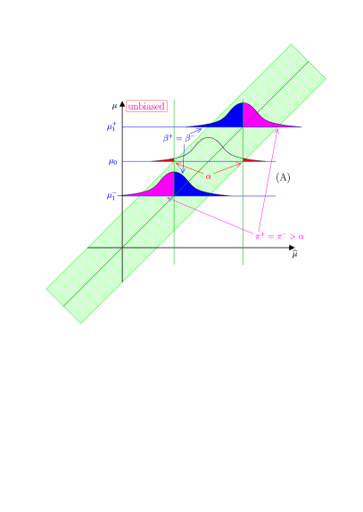
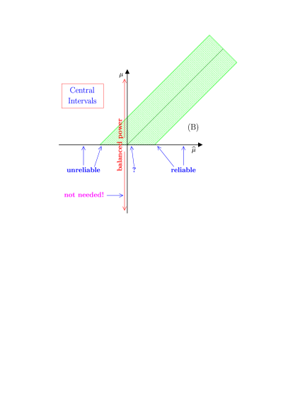
Figure 1: A: Power $\pi$ in the Central Intervals method for an estimator $\widehat{\mu}$ of $\mu$ that has a Gaussian distribution. B: Reliability of the Confidence Intervals obtained with the Central Intervals method for a bounded $\mu\geq 0$. See text for details.

From Fig. 1A one can see that the power corresponding to alternative hypotheses $\mu_{1}^{-}$ and $\mu_{1}^{+}$, respectively smaller and larger than the null hypothesis $\mu_{0}$, is equal. The Central Intervals method produces the most reliable results in the case of an unbounded $\mu$, because the power is perfectly balanced. Problems arise if one considers the measurement of a bounded quantity $\mu$. As illustrated in Fig. 1B for the case of a bounded $\mu\geq 0$, the balanced power in the Central Intervals method is not appropriate. Indeed, a high power to test $\mu_{0}$ against $\mu_{1}^{-}<\mu_{0}$ when $\mu_{0}$ is near the boundary is not needed, because the alternatives $\mu_{1}^{-}<\mu_{0}$ are limited. As a result, the Central Intervals method produces in this case clearly unreliable Confidence Intervals if the value of $\widehat{\mu}_{\mathrm{obs}}$ lies on the left-hand side of Fig. 1B. Sometimes the Confidence Interval can be empty, giving no information. Sometimes one can get a very stringent upper limit, much smaller than the exclusion potential of the experiment [4, 7]. This possibility is very dangerous, because it can lead to wrong conclusions if interpreted in inappropriate ways. In any case it gives no useful information on the value of $\mu$.

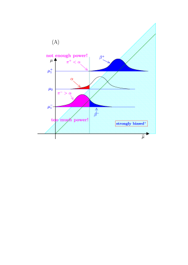
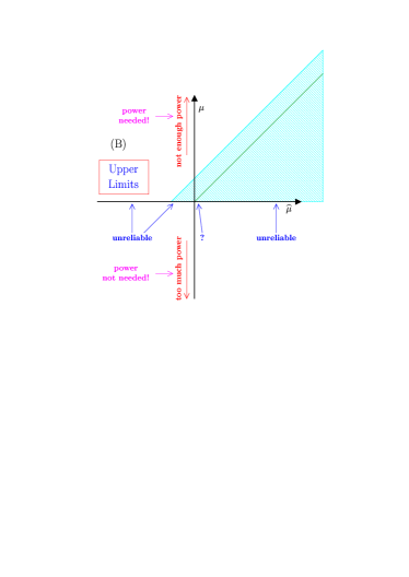
Figure 2: A: Power $\pi$ in the Upper Limits method for an estimator $\widehat{\mu}$ of $\mu\geq 0$ that has a Gaussian distribution. B: Reliability.

In the past the Upper Limits method was rather popular. Figures 2A and 2B show that the Upper Limits method is actually worse than the Central Intervals method because it is biased in the wrong direction. As a consequence, it produces limits that are practically always unreliable, except maybe when by chance $\widehat{\mu}_{\mathrm{obs}}\simeq 0$.

The method biased in the right direction that has been proposed first is the Unified Approach of Feldman and Cousins [4], which, as illustrated in Fig. 3A, gives more power to test $\mu_{0}$ against $\mu_{1}^{+}>\mu_{0}$ than to test $\mu_{0}$ against $\mu_{1}^{-}<\mu_{0}$ when $\mu_{0}$ is near the boundary. However, the bias is still insufficient to produce reliable results if $\widehat{\mu}_{\mathrm{obs}}\ll 0$: from Fig. 3B one can see that when $\widehat{\mu}_{\mathrm{obs}}\ll 0$ the Confidence Interval gives an upper limit for $\mu$ that is unphysically too small [5, 8, 2, 9, 10], much smaller than the exclusion potential of the experiment [4, 7].

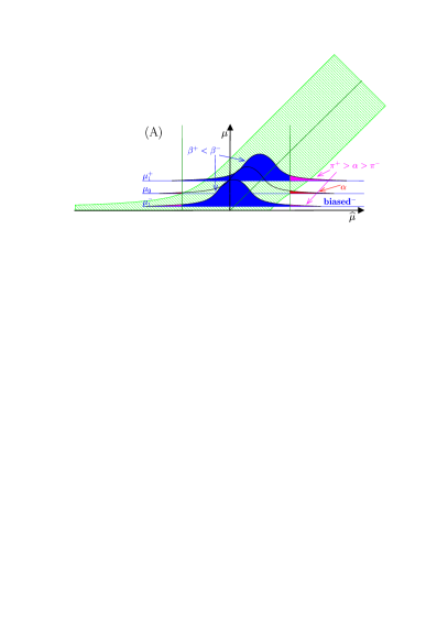
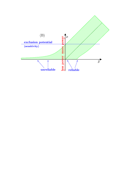
Figure 3: A: Power $\pi$ in the Unified Approach for an estimator $\widehat{\mu}$ of $\mu\geq 0$ that has a Gaussian distribution. B: Reliability.

Figure 4A illustrates the calculation of the power in the Maximum Likelihood Estimator method proposed independently by Ciampolillo in Ref. [1] and Mandelkern and Schultz in Ref. [2]. In this method the estimator of $\mu$ is not $\widehat{\mu}$, but the maximum likelihood value $\mu^{*}$ of $\mu$. Since the range of $\mu^{*}$ is equal to the range of $\mu$, the estimate $\mu^{*}_{\mathrm{obs}}$ always lies in the physical range of $\mu$. In the case of a Gaussian distribution for $\widehat{\mu}$ illustrated in Fig. 4A, $\mu^{*}=\widehat{\mu}$ for $\widehat{\mu}\geq 0$ and $\mu^{*}=0$ for $\widehat{\mu}\leq 0$. Therefore, as shown in Fig. 4A, the upper limit for $\mu$ obtained for any $\widehat{\mu}_{\mathrm{obs}}<0$ is equal to the upper limit obtained for $\widehat{\mu}_{\mathrm{obs}}=0$.

As one can see from Fig. 4A, the Maximum Likelihood Estimator method has optimal bias. As a consequence, this method produces reliable results for any value of $\widehat{\mu}_{\mathrm{obs}}$, as shown in Fig. 4B.

Let us emphasize that the bias is needed near the boundary and both the Maximum Likelihood Estimator method and the Unified Approach produce Confidence Intervals that practically coincide with those obtained with the Central Intervals method when $\widehat{\mu}_{\mathrm{obs}}\gg 0$.

In conclusion, we have shown that the Maximum Likelihood Estimator method [1, 2] have optimal power in the case of measurement of a bounded quantity and produces always reliable Confidence Intervals. For these reasons, it should be preferred over the Unified Approach [4], which is however better than the Central Intervals method. Worse of all is the method of Upper Limits.

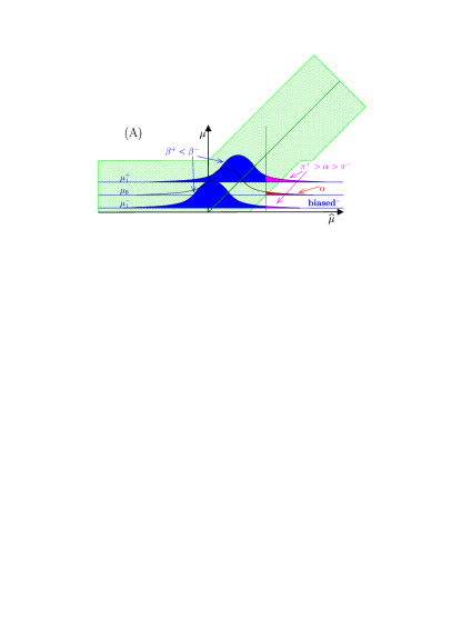
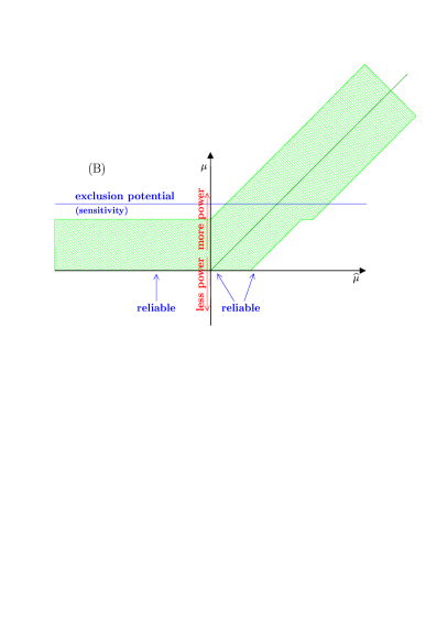
Figure 4: A: Power $\pi$ in the Maximum Likelihood method for an estimator $\widehat{\mu}$ of $\mu\geq 0$ that has a Gaussian distribution. B: Reliability.

References

- [1] S. Ciampolillo, Nuovo Cim. A111, 1415 (1998).
- [2] M. Mandelkern and J. Schultz, J. Math. Phys. 41, 5701 (2000), hep-ex/9910041.
- [3] A. Stuart, J.K. Ord and S. Arnold, Kendall’s Advanced Theory of Statistics, Vol. 2A, Classical inference and the linear model Sixth Edition, Oxford University Press, 1999.
- [4] G. J. Feldman and R. D. Cousins, Phys. Rev. D57, 3873 (1998), physics/9711021.
- [5] C. Giunti, Phys. Rev. D59, 053001 (1999), hep-ph/9808240.
- [6] C. Giunti and M. Laveder, Nucl. Instrum. Meth. A480, 763 (2002), hep-ex/0011069.
- [7] C. Giunti and M. Laveder, Mod. Phys. Lett. 12, 1155 (2001), hep-ex/0002020.
- [8] B. P. Roe and M. B. Woodroofe, Phys. Rev. D60, 053009 (1999), physics/9812036.
- [9] C. Giunti, CERN “Yellow” Report CERN 2000-005, 63 (2000), hep-ex/0002042, Proceedings of the Workshop on Confidence Limits at CERN, 17-18 January 2000, edited by F. James, L. Lyons, Y. Perrin. http://preprints.cern.ch/cernrep/2000/2000-005/2000-005.html.
- [10] P. Astone and G. Pizzella, CERN “Yellow” Report CERN 2000-005, 199 (2000), hep-ex/0002028, Proceedings of the Workshop on Confidence Limits at CERN, 17-18 January 2000, edited by F. James, L. Lyons, Y. Perrin. http://preprints.cern.ch/cernrep/2000/2000-005/2000-005.html.