FERMILAB-FN-720

nuhep-exp/2002-03

Physics Potential at FNAL with Stronger Proton Sources

G. Barenboim^a, A. de Gouvêa^a, T. Dombeck^a,

N. Grossman^a, D. Harris^a, D. Michael^b, M. Szleper^c,

M. Velasco^c, S. Werkema^a

^aFermi National Accelerator Laboratory
P.O. Box 500, Batavia, IL 60510, USA
^b California Institute of Technology High Energy Physics,
Charles C. Lauritsen Laboratory, Pasadena, CA 91125, USA
^c Northwestern University
Department of Physics & Astronomy
2145 Sheridan Rd, Evanston, IL 60208, USA

This document is the second in a series of reports on the exciting physics that would be accessible at Fermilab in the event of an upgraded proton source. Where the first report covered a broad range of topics, this report focuses specifically on three areas of study: there are brief discussions on the new measurements one could make in both the neutron and anti-proton sectors, and then a detailed discussion of what could be achieved in the neutrino oscillation sector using an upgraded proton source to supply the NuMI beamline with more protons. If one places a new detector optimized for $\nu_{e}$ appearance at a new location slightly off the axis defined by the MINOS experiment, that new experiment would be ideal for making the next important steps in lepton flavor studies, namely, the search for $\nu_{\mu}\to\nu_{e}$ at the atmospheric mass splitting, and CP violations. The report concludes with a summary of proton economics and demands for increased proton intensity for the Booster and Main Injector: what the proton source at Fermilab can currently supply, and what adiabatic changes could be implemented to boost the proton supply on the way from here to a proton driver upgrade.

1 Goals and Charge

In January of 2001 a study on the physics potential of a new high intensity proton source facility ($\sim$0.5MW)[1] at Fermilab was requested by Mike Shaevitz. The idea was that such a facility could be the basis of a high quality U.S. based physics program, to be operated between the second half of this decade and the commissioning of the next major U.S. facility. By that summer, the working group had concluded that a rich and coherent program in “Flavor Physics” could be achieved[2], and that the Proton Driver (PD) would have a large impact on a variety of programs that are currently being pursued at Fermilab using the existing machines as well as the potential for new facilities. Experiments that would clearly benefit from a new PD included among others, the neutrino experiments covering both the hot topic of oscillations (e.g. Minos and BooNE) as well as non-oscillation physics. The possible new facilities are a neutron spallation source and a high intensity low energy muon source. These facilities would be competitive and complementary to other existing or proposed facilities, and would attract new users to Fermilab.

In December 2001 by Mike Shaevitz and Steve Holmes requested to re-invigorate the PD studies. Steve Holmes was interested in pursuing an updated machine study with the goal of having a new design in time for the ICFA Workshop on High Intensity High Brightness Hadron Beams that took place at Fermilab on April 8-12 of 2002[3]. Mike Shaevitz requested a strong and detailed updated physics study to be presented first at the same ICFA workshop and have final report by the PAC scheduled for June, 2002.

The new goals were to identify a range of accelerator configurations that could provide 0.5-2 MW of average beam power at 8-120 GeV, describe the physics program that could be supported and identify required beamlines and detectors. The scope of this study was to be limited to three strong physics topics that could be pursued with a new PD. Conceptual designs for the beam lines, targets and detectors were required, as well as consideration of a physics program based on both a stand alone source and an upgraded Main Injector.

This document is the response to the request from Shaevitz and Holmes from the physics working group. Even though we focused on the physics program, we also include a discussion of proton economics at Fermilab in order to shows that the physics goals considered will require a significant increase in the proton resources at Fermilab. Only with an upgraded proton source, such as the one described in [4] would we be able to achieve the physics objectives listed here, and fully capitalize on the Fermilab program already in place.

2 Summary

There are many benefits that would come from a Proton Driver upgrade. In this document we focus on three physics areas: neutrino oscillations, static neutron properties and CPT tests with anti-protons. In all three areas Fermilab can make unique and important physics contributions.

However, there is no doubt that neutrino physics is going through a revolutionary moment, and that neutrino masses and mixings are already giving us new insights into the origin of flavor. In addition, given the evidences for neutrino mass, leptogenesis is gaining momentum as the origin of cosmic baryon asymmetry, and therefore CP violation in the lepton sector must be tested. For these reasons, and many others, we have made our main emphasis neutrino oscillation physics, which is the first topic covered. In the near future, at Fermilab we will definitively open (or close) the door to new physics [5] in the neutrino sector by confirming (or not) the LSND anomaly [6] with MiniBooNE data [7]. In case that LSND is confirmed we need even more protons than what we have available in the current Booster. The physics case that should follow, in the case that MiniBoone confirms LSND and in the availability of a new PD was already discussed in detailed in our previous report [2]. Here we focus on the experiments that are critical should LSND not be confirmed.

More detailed studies of the other two topics, static neutron properties and CPT tests with anti-protons, should come at a later date.

Neutrino Oscillations: We describe in detail a proposal for an off-axis neutrino experiment utilizing the NuMI beamline. As we will show in the following sections, this and the next generation of neutrino experiments can measure most of the leptonic mixing angles and mass-squared differences from which it will be possible to infer the neutrino mass hierarchy. The detector design will ensure the observation of $\nu_{\mu}\rightarrow\nu_{e}$ appearance, if the last unmeasured angle in the leptonic mixing matrix ($|U_{e3}|^{2},\theta_{13}$) is large enough. Depending on the outcome, it will be possible to observe CP violations, if they exist, by taking data with an anti-neutrino beam. At that stage of the program, the key to success is the higher proton flux afforded by the Proton Driver. We show that this project can be staged to match Fermilab resources.

Neutron Static Properties: The electric dipole moment (EDM) of the neutron could provide a window on new physics, as has been appreciated for many years. The current measurements constrain important parameters in Supersymmetry, for example. The next generation of experiments will likely require a pulsed source of neutrons in order to control systematics. As observed already in earlier reports on the proton driver [2, 1], a world class spallation neutron source could be built at Fermilab utilizing the Proton Driver which would have unique capabilities and compliment other facilities elsewhere.

CPT Tests with Anti-protons: General interest in tests of CPT symmetry is growing as experimental efforts improve and theoretical possibilities for CPT violation are recognized. Some of the most important work has been done with anti-protons at CERN, using the AD (‘Anti-proton Decelerator’). This program will be terminated, however, as CERN focuses its resources on the LHC. At FNAL we already have an anti-proton source, therefore Fermilab is good candidate for the next generation of anti-proton and anti-Hydrogen experiments. The program can start with the current facilities, and ultimately be enhanced with the Proton Driver.

2.1 Neutrino Program

An off-axis experiment in combination with a PD upgrade would be capable of observing both $\nu_{\mu}\rightarrow\nu_{e}$ and $\nu_{\mu}\rightarrow\nu_{\tau}$ appearance, and $\nu_{\mu}$ disappearance. In addition, the experiment will be able to measure precisely the atmospheric parameters, measure or make stringent exclusions of $|U_{e3}|^{2}~{}(\theta_{13})$, and ultimately search for CP violation in the lepton sector and determine the mass hierarchy once the new Proton Driver becomes available. Several detector technologies with the required physics specifications are available at varying cost and level of complexity. Modest changes are required for the NuMI beam line, which is already approved and currently under construction.

We describe a search for neutrino oscillations in the atmospheric neutrino allowed region. The OFF-MINOS (Off-axis detector – Main Injector Neutrino Oscillation Search) program could have two phases. The first phase assumes a total of 125 kTon/years, and we will be able to:

• Extend the search for $\nu_{\mu}\rightarrow\nu_{e}$ appearance for a factor bigger than 20 past the current experimental bound at a three sigma level.

• Obtain an exclusion for $\nu_{\mu}\rightarrow\nu_{e}$ appearance for $|U_{e3}|^{2}>0.0015$, at a two sigma level. This is approximately twenty times beyond current limits and almost an order of magnitude better than the MINOS expectation if no signal is observed.

• Precision measurements of atmospheric $\nu$ parameters. Despite the large suppression we expect more than 10 $\nu_{\mu}C\rightarrow\mu+X$ fully reconstructed events per kTon/year. After the full program is completed we should have 1% measurement of the atmospheric oscillation parameters.

• The search for $\nu_{\mu}\rightarrow\nu_{\tau}$ appearance will be inferred from measurements of the neutral current rate, which would constrain the sterile neutrinos sector.

The actual program for a second phase will depend on the outcome of the first stage. If $\nu_{\mu}\rightarrow\nu_{e}$ appearance were discovered, then one may devote as much as 300 kTon/year of running time to anti-neutrinos. (A longer exposure is required to compensate for the smaller cross section.) At this stage the new Proton Driver is crucial. In this case the goals are:

• Search of CP violation in the lepton sector, and measurement of the CP-phase.

• Determination of the mass hierarchy.

If $\nu_{\mu}\rightarrow\nu_{e}$ appearance were not observed in the first stage, then the search for $\nu_{\mu}\rightarrow\nu_{e}$ would continue.

The OFF-MINOS experiment should be taking data by 2007 in order to be concurrent with the JHF-to-SuperK program. Using a modular design, the OFF-MINOS detector could be staged according to the availability of resources. The final detector design is still under discussion, but it is clear that we need detectors that will provide high reconstruction efficiencies for charged $\nu_{e}$ current events ($\epsilon\geq 35\%$), while keeping the neutral current background below the two per mil level. The detector should be located 9-10 km from the beam axis and at a baseline between 735-900 km from the neutrino source.

This experiment is compatible with the MINOS program.

The OFF-MINOS experiment represents an important and unique opportunity to take full advantage of the NuMI investment and expand the neutrino oscillation program at Fermilab. A Proton Driver will be crucial to reach the ultimate goal of neutrino oscillations, CP-violations.

2.2 Neutron Program

The new Proton Driver [1] will give a proton beam in the MW range that could produce a world-class spallation neutron source using a small fraction (4/30) of its total power. An intense room-temperature neutron source [8, 9], suitable for a wide variety of fundamental physics experiments [10, 11], can be made at FNAL by optimizing the target and moderator system for long pulses ($\Delta\tau\simeq 400\mu$s). This source will be complimentary to the short-pulse sources ($\Delta\tau<40\mu$s) optimized for materials research such as the SNS at ORNL and JHF in Japan.

The advantages of a long-pulse neutron source include [9, 10, 11]: (1) high peak intensities that can provide the most intense long-wavelength neutron sources, (2) the use of Time-Of-Flight (TOF) techniques to measure energies, and (3) reduced backgrounds because of the favorable duty factor. This would permit the investigation of a number of important particle physics questions such as time-symmetry violation, baryon number conservation, parity-nonconservation in strong interactions, right-handed weak currents, and quantum mechanics at the macroscopic scale [11].

The primary topic, in the view of colleagues at Argonne and Fermilab, is the measurement of the neutron electric dipole moment (EDM).

Experimental discovery of CP violation in flavor-conserving channels would provide a clear indication of new physics at the electroweak scale. This stimulates continuing experimental efforts to detect EDM’s in elementary particles and heavy atoms [12]. The extraordinary precision $d_{n}<6\,\times\,10^{-26}$ e-cm [13], obtained in measurements of the EDM of the neutron, allows us to probe energy scales inaccessible in direct collider experiments.

There have been two methods to search for the neutron Electric Dipole Moment. One pioneered by Norman Ramsey uses an external electric field to couple the EDM, and the second pioneered by Clifford Shull uses the atomic electric fields during Bragg scattering in a crystal. In both cases the EDM precesses in the electric field in the same manner that a magnetic dipole precesses in a magnetic field and both experiments search for evidence of this precession using magnetic resonance techniques. As the amount of precession is inversely proportional to the time spent in the electric field, the sensitivity of the Ramsey method has been improved through the use of ultracold neutrons that can be stored in material bottles for many minutes [12, 14]. Atomic electric fields are much larger than those generated in the laboratory, however the time spent in the field is much smaller. Increasing the sensitivity of this method depends on the use of multiple Bragg scatters made possible by the use of perfect silicon crystals [15]. The systematic errors differ for each method and as the EDM measurement is important to particle physics it is necessary to have confirmation of a positive result.

The current attempt to improve upon the Ramsey method involves a milli-Kelvin bath of liquid helium that effectively cools the neutrons and traps them [14]. The method uses neutrons of about 1 meV with an acceptance bandwidth of $<1~{}$meV. The hope is to perform the magnetic resonance and detection in the same vessel that contains the liquid helium. Estimates made for an ILL reactor source show a possible improvement of three orders of magnitude in the EDM sensitivity. However, from preliminary tests performed at the NIST reactor [16], it appears that backgrounds generated by the higher energy neutrons in the beam is a serious problem. One solution would be to mount the experiment at a pulsed source and use TOF to select only the “useful” neutrons. A long-pulse source will not provide the full 1 meV TOF resolution, but it is estimated that even a 100 meV resolution would provide orders of magnitude improvement in the S/N ratio.

In the crystal EDM experiment, thousands of successive Bragg scatters have been demonstrated in perfect silicon crystals [17] suggesting that this experiment may also provide up to two orders of magnitude improvement in the EDM sensitivity. However, the experimental method requires a control measurement to isolate the EDM [15]. One way to provide this would be to use 1.92 A neutrons at the same time as 3.84 A neutrons because both will Bragg scatter in silicon. Each wavelength responds differently to an EDM precession and their effects can be separated at a pulsed source using TOF.

In either case the first thing that needs to be done is to validate the model currently under consideration to produce a spallation source starting from 8 GeV protons [8]. This first step can be made at the booster abort area, and a proposal is under preparation.

2.3 P-bar Program

As discussed in the Proton Driver physics study [2], the addition of the Recycler Ring to the Fermilab accelerator complex provides an opportunity to continue the program of $\bar{p}$ physics with the Anti-proton Source Accumulator. We have found that the Proton Driver will have a negligible impact on luminosity delivered to the collider, while significantly increasing the luminosity received by an experiment at the Accumulator.

The operational scenario for the $\bar{p}$ source presented here utilizes the Recycler Ring as an anti-proton bank from which the colliders makes ‘withdrawals’ as needed to maintain the required luminosity in the Tevatron. The Accumulator is only needed to re-supply the bank between withdrawals. When the $\bar{p}$ stacking rate is sufficiently high, and the luminosity requirements of the Collider experiments are sufficiently low, there will be time between Collider fills and subsequent refilling of the recycler to deliver beam to an experiment in the Accumulator. In the scenario described in [2], the impact of the Accumulator experiment on the luminosity delivered to the Collider experiments is very small. If the Run II anti-proton stacking rate goals are met, the operational conditions required for running Accumulator based experiments will be met during the BTeV era. A simple model of the operation of the Fermilab accelerator complex for BTeV and an experiment in the Collider has been developed [2]. The model makes predictions of the rate at which luminosity is delivered to BTeV and an Accumulator experiment. The impact of the Proton Driver is incorporated into the model as a multiplicative factor that is applied to the Accumulator base stacking rate.

The model generates Collider stores and Accumulator stores according to the following priorities:

• 1st priority: Put a store in the Tevatron for BTeV

• 2nd priority: Stack $\bar{p}$’s into the Recycler until there are sufficient $\bar{p}$’s for two Collider stores

• 3rd priority Stack and decelerate $\bar{p}$’s for the Accumulator experiment

The model accumulates the integrated luminosity delivered to BTeV and to the Accumulator experiment. For the results reported here, the model simulated Collider and Accumulator running over a period of 200 days. The model’s determination of the luminosity delivered to the Accumulator experiment is based on measurements made during the 2000 run of Fermilab experiment E835.

Two separate model runs were done - one with and one without an enhancement of the stacking from the Proton Driver. The model assumes that the Proton Driver will increase the Accumulator base stacking rate by a factor of three. The results of these runs are summarized in Table 1.

Table 1: Model Results for $\bar{p}$ production.

	No Proton Driver	Proton Driver Enhanced
BTeV Up Time	191.71 days     95.85%	192.75 days    96.32%
Acc. Expt. Up Time	64.41 days    32.21%	126.55 days    63.24%
Collider Stacking	112.58 days    56.29%	41.56 days    20.77%
Accumulator Stacking	7.63 days    3.82%	11.35 days    5.67%
BTeV $\int Ldt$	92.80 pb-1/week	93.44 pb-1/week
Acc. Expt. $\int Ldt$	5.84 pb-1/week	11.47 pb-1/week

There are two significant findings from this analysis. The first is that, to the extent that the performance of the Fermilab accelerator complex is characterized by the above model parameters, it is possible to run an experiment in the Accumulator without significantly impacting the collider program. The second finding is that the Proton Driver will have a negligible impact on luminosity delivered to the collider, while significantly increasing the luminosity received by an Accumulator experiment.

3 NuMI Based Neutrino Oscillation Program Towards a PD Upgrade

There are several outstanding issues in the field of neutrino oscillation measurements – is the three generation framework correct? Are there sterile neutrinos? Are any of the mixing angles exactly 0 or exactly $\pi/4$? Is there CP violation in the lepton sector? While we would like to eventually answer all of these questions, many agree that the next big goal beyond the current round of approved experiments is to search for evidence of $\nu_{\mu}\to\nu_{e}$ at the atmospheric mass splitting, which would tell us if the one completely unmeasured mixing angle, $\theta_{13}$, is non-zero.

If $\theta_{13}$ is measured to be non-zero, then this opens up the way for the next very interesting steps, namely, exploiting matter effects to determine the neutrino mass hierarchy, and, assuming the solar neutrino solution is described by LMA, a search for CP violation in the lepton sector. In other words, as well as being interesting in its own right, discovery of a non-zero $\theta_{13}$ defines the next interesting things to measure – it is not the end of the story, merely the beginning.

Given these assumptions, the next steps for this community are clear: one must first focus our efforts on finding evidence for a non-zero $\theta_{13}$, but keep in mind that ultimately we will want to make much higher precision measurements. To understand matter effects and the mass hierarchy we will want to measure $\nu_{\mu}\to\nu_{e}$ in both the neutrino and anti-neutrino channels. Finally, given the long history of “anomalies” seen in this field (atmospheric, solar, LSND), we think it is important for there to be a measurement of $\theta_{13}$ at more than one baseline and preferably with more than one detector technology.

In this section we describe in detail how an off-axis neutrino program based on NuMI can address these issues. It could start with NuMI in its current design and configuration. Once the Proton Driver becomes available, this program would go on to test for CP violation and to measure matter effects. We have organized this section as follows: First, we briefly review the neutrino mixing matrix and oscillation probabilities, and describe the current knowledge of neutrino masses and mixing angles, and what the near term series of experiments should tell us. In Sec. 3.2, we describe the off-axis neutrino beam, and discuss where an off-axis detector (Sec. 3.3) should be located in order to maximize its physics capabilities. In Sec. 3.4, we describe one example of a fine-grained calorimeter which could serve as a $\nu_{e}$ detector, and discuss its reconstruction efficiencies and strategies for reducing the number of background events in order to make a realistic assessment of the physics capabilities of the proposed program. In Sec. 3.5-3.7, we discuss the physics capabilities of such a setup, for different values of the solar mass-squared difference.

3.1 Introduction

The SuperKamiokande experiment [18] observes an angular-dependent (and energy-dependent) suppression of the atmospheric muon-type neutrino flux, confirming with much higher precision the deficit seen by previous experiments [19]. The best interpretation for this puzzle is that some of the $\nu_{\mu}$’s transform into $\nu_{\tau}$’s. On a different front, solar neutrino experiments [20, 21, 22] have consistently measured $\nu_{e}$ fluxes which are significantly smaller than those predicted by theory [23]. Indeed, recent results from the SNO experiment [22] imply, at the five sigma level, that there are active neutrinos other than $\nu_{e}$ ($\nu_{\mu}$ and/or $\nu_{\tau}$) coming from the Sun. Finally, the LSND Collaboration [6] has reported an anomalous flux of $\bar{\nu}_{e}$, which may be interpreted as evidence for $\bar{\nu}_{\mu}\leftrightarrow\bar{\nu}_{e}$ oscillations. This experimental evidence has not yet been independently confirmed, but will be put to the test in the near future by MiniBooNE [7].

Neutrino oscillations provide, by far, the simplest and most elegant solution to two out of three of these puzzles. Of course, to accommodate all three puzzles one would have to invoke even more exotic processes, since with three generations of neutrinos there can only be two independent mass splittings, and the three signatures imply three very different mass splittings. It should be emphasized, however, that less standard solutions [24] cannot yet be discarded.

Neutrino oscillations (and other types of new physics in the neutrino sector) can also be potentially observed in terrestrial neutrino experiments, by studying, for example, the flux of $\bar{\nu}_{e}$ coming from nuclear reactors [25] or studying the $\nu_{\mu}$ flux from pion or muon decays [26]. The current results significantly constrain the neutrino oscillation parameter space, as will be discussed in more detail in the next subsection. If the LSND anomaly is confirmed (and is indeed a consequence of neutrino masses and mixing), a more complicated neutrino sector is required. This intriguing possibility will not be considered here, but the implications for future experiments were discussed in reference [2]

Henceforth we will assume that active neutrino oscillations are the solution to the solar and atmospheric neutrino results. In this case the standard model is augmented by at least seven (and possibly nine) new parameters. These are three neutrino masses, three mixing angles and one Dirac phase, which define the neutrino mixing matrix, and two additional Majorana phases, which exist only if the neutrinos are Majorana particles. Neutrino oscillation experiments, can probe six of these parameters: two mass differences, three angles, and the Dirac phase.

3.1.1 Neutrino Oscillation Formalism

The presence of non-zero masses for the light neutrinos introduces a leptonic mixing matrix, $U$, analogous to the well-known CKM quark mixing matrix, and which we know already would be far from diagonal. The matrix $U$ connects the neutrino flavor eigenstates with the mass eigenstates:

$$|\nu_{\alpha}\rangle=\sum_{i}U_{\alpha i}|\nu_{i}\rangle,$$ (1)

where $\alpha$ denotes the active neutrino flavors, $e,\ \mu$ or $\tau$, while $i$ runs over the mass eigenstates. It is “traditional” to define the mixing angles $\theta_{12,13,23}$ in the following way:

$$\tan^{2}\theta_{12}\equiv\frac{|U_{e2}|^{2}}{|U_{e1}|^{2}},~{}~{}~{}\tan^{2}\theta_{23}\equiv\frac{|U_{\mu 3}|^{2}}{|U_{\tau 3}|^{2}},~{}~{}~{}\sin^{2}\theta_{13}\equiv|U_{e3}|^{2},$$ (2)

while

$$\Im(U_{e2}^{*}U_{e3}U_{\mu 2}U_{\mu 3}^{*})\equiv\sin\theta_{12}\cos\theta_{12}\sin\theta_{23}\cos\theta_{23}\sin\theta_{13}\cos^{2}\theta_{13}\sin\delta$$ (3)

defines the CP-odd phase $\delta$. For Majorana neutrinos, $U$ contains two further multiplicative phase factors, but these are invisible to oscillation phenomena.

In order to relate the mixing angles and mass-squared differences to the parameters constrained by experiments, it is convenient to define the neutrino masses such that $m_{1}^{2}<m^{2}_{2}$ and $\Delta m^{2}_{12}<|\Delta m^{2}_{13,23}|$, where $\Delta m^{2}_{ij}\equiv m_{j}^{2}-m_{i}^{2}$ (the data, in fact, point to $\Delta m^{2}_{12}\ll|\Delta m^{2}_{13,23}|$). With this definition, the “solar angle” $\theta_{\odot}\simeq\theta_{12}$, while the atmospheric angle $\theta_{\rm atm}\simeq\theta_{23}$. Furthermore, reactor experiments constrain $|U_{e3}|^{2}$. The solar mass-squared difference $\Delta m^{2}_{\odot}=\Delta m^{2}_{12}$, while the atmospheric mass-squared difference is $\Delta m^{2}_{\rm atm}=|\Delta m^{2}_{13}|\simeq|\Delta m^{2}_{23}|$. It is important to note that $m_{3}^{2}$ can be either larger or smaller than $m_{1}^{2},m_{2}^{2}$.

The oscillation probability $P(\nu_{\alpha}\rightarrow\nu_{\beta})$ is given by the absolute square of the overlap of the observed flavor state, $|\nu_{\beta}\rangle$, with the time-evolved initially-produced flavor state, $|\nu_{\alpha}\rangle$. In vacuum, it yields the well-known result:

$$\begin{array}[]{rl}P(\nu_{\alpha}\rightarrow\nu_{\beta})=&\left|\langle\nu_{\beta}|e^{-iH_{0}L}|\nu_{\alpha}\rangle\right|^{2}=\sum_{i,j}U_{\alpha i}U^{*}_{\beta i}U^{*}_{\alpha j}U_{\beta j}e^{-i\Delta m^{2}_{ij}L/2E}\\[7.22743pt] =&P_{\rm CP-even}(\nu_{\alpha}\rightarrow\nu_{\beta})+P_{\rm CP-odd}(\nu_{\alpha}\rightarrow\nu_{\beta})\;.\\[7.22743pt] \end{array}$$ (4)

The CP-even and CP-odd contributions are

$$\begin{array}[]{rl}P_{\rm CP-even}(\nu_{\alpha}\rightarrow\nu_{\beta})=&P_{\rm CP-even}(\bar{\nu}_{\alpha}\rightarrow\bar{\nu}_{\beta})\\[7.22743pt] =&\delta_{\alpha\beta}-4\sum_{i>j}\ Re\ (U_{\alpha i}U^{*}_{\beta i}U^{*}_{\alpha j}U_{\beta j})\sin^{2}({{\Delta m^{2}_{ij}L}\over{4E}})\\[7.22743pt] P_{\rm CP-odd}(\nu_{\alpha}\rightarrow\nu_{\beta})=&-P_{\rm CP-odd}(\bar{\nu}_{\alpha}\rightarrow\bar{\nu}_{\beta})\\[7.22743pt] =&2\sum_{i>j}\ Im\ (U_{\alpha i}U^{*}_{\beta i}U^{*}_{\alpha j}U_{\beta j})\sin({{\Delta m^{2}_{ij}L}\over{2E}})\\[7.22743pt] \end{array}$$ (5)

such that

$$P(\bar{\nu}_{\alpha}\to\bar{\nu}_{\beta})=P(\nu_{\beta}\to\nu_{\alpha})=P_{\rm CP-even}(\nu_{\alpha}\rightarrow\nu_{\beta})-P_{\rm CP-odd}(\nu_{\alpha}\rightarrow\nu_{\beta}),$$ (6)

where, by CPT invariance , $P(\nu_{\alpha}\to\nu_{\beta})=P(\bar{\nu}_{\beta}\to\bar{\nu}_{\alpha})$. In vacuum the CP-even and CP-odd contributions are even and odd, respectively, under time reversal: $\alpha\leftrightarrow\beta$.

If the neutrinos propagate in matter, these expressions are modified, because of the additional forward scattering process of electron-type neutrinos and anti-neutrinos off of electrons in matter. The propagation of neutrinos through matter is described by the evolution equation

$$i{d\nu_{\alpha}\over dt}=\sum_{\beta}\left[\left(\sum_{j}U_{\alpha j}U_{\beta j}^{*}{m_{j}^{2}\over 2E_{\nu}}\right)+{A\over 2E_{\nu}}\delta_{\alpha e}\delta_{\beta e}\right]\nu_{\beta}\,,$$ (7)

where $A/(2E_{\nu})$ is the amplitude for coherent forward charged-current scattering of $\nu_{e}$ on electrons,

$$A=2\sqrt{2}G_{F}N_{e}E_{\nu}=1.52\times 10^{-4}{\rm\,eV^{2}}Y_{e}\rho({\rm\,g/cm^{3}})E({\rm\,GeV}).\,$$ (8)

For anti-neutrinos, $A$ is replaced with $-A$, and $U$ with $U^{*}$. Here $Y_{e}$ is the electron fraction and $\rho(t)$ is the matter density. For neutrino trajectories through the earth’s crust, the density is typically of order 3 g/cm³, and $Y_{e}\simeq 0.5$. For propagation through matter of constant density, the transition probabilities can be written in the form Eq.( 5), but by modifying the mass splitting and mixing angle by a constant which is a function of $A$, and $\Delta m_{13}^{2}$. The change due to matter effects as a function of baseline is shown in Fig. 1.

Figure 1: Transition probabilities for neutrinos (green, top curve) and anti-neutrinos (blue, bottom curve) in matter and vacuum (red, middle curve) as function of the distance for 2 GeV, $\Delta m^{2}_{13}=3\cdot 10^{-3}~{}{\mbox{eV}}^{2}$ (normal hierarchy), $\theta_{\rm atm}=\pi/4$, $\Delta m^{2}_{\odot}=1\times 10^{-4}$ eV², $\theta_{\odot}=\pi/6$, $|U_{e3}|^{2}=0.04$, and $\delta=0$.

Long baseline (i.e. $>500km$) neutrino experiments therefore are sensitive to matter effects, where the size of the effect is strongly dependent on the baseline length and neutrino energy. Some unknowns related to the neutrino mass pattern can be addressed with the “help” of the matter effects. As alluded to before, the current data leave us with two alternatives for the spectrum of the three active neutrino species: a “normal” neutrino mass hierarchy or an “inverted” neutrino mass hierarchy. In the case of a “normal” mass hierarchy, the “solar pair” of states is lighter than $\nu_{3}$, i.e. $m_{3}>m_{2},m_{1}$. In the case of inverted hierarchy, the states of the solar pair are heavier than $\nu_{3}$, i.e. $m_{3}<m_{2}\simeq m_{1}$. The key difference between these two hierarchies is then that, in the normal hierarchy, the small $U_{e3}$ admixture of $\nu_{e}$ is in the heaviest state whereas in the inverted hierarchy, this admixture is in the lightest state. The difference between both schemes is parameterized by the sign of $\Delta m^{2}_{23}$. A positive $\Delta m^{2}_{23}$ is defined as a normal hierarchy.

In going from $\nu$ to $\overline{\nu}$, there are matter-induced CP- and CPT- odd effects associated with the change $A\rightarrow-A$. The additional change U $\rightarrow$ U^∗ introduces further effects (this is the “genuine” CP-violation), which are usually subleading. Note that the matter effects depend on the interference between the different flavors and on the relative sign between $A$ and $\Delta m^{2}_{23}$. As a consequence, an experimental distinction between the propagation of $\nu$ and $\overline{\nu}$ (the sign of $A$) can determine the sign of $\Delta m^{2}_{23}$.

The Standard Model can be extended to incorporate neutrino masses in a variety of ways. Many theories beyond the minimal model also lead to non standard neutrino interactions [27]. These include most models of generating neutrino masses, such as the simplest seesaw type schemes, supergravity $SO(10)$ unified theories, models of low energy supersymmetry with broken R-parity as well as some radioactive models of neutrino masses.

Long baseline neutrino experiments have a reasonable potential for probing non standard neutrino matter interactions as well as some kinds of new physics, specially if a non zero CP violating effect is detected. The role of a long baseline experiment in testing this kind of new physics is complementary to efforts to probe similar flavour changing effects in the charged lepton sector while being model independent.

CP violating observables are particularly sensitive to new physics because they are not necessarily as suppressed by the small mass differences and mixing angles as the standard contributions. Even more, the dependence on the distance between the source and the detector is in general different, and this might help in disentangling standard effects from the new ones.

If one tries to incorporate the LSND signal only using oscillations between active flavors, all data can be consistently fit by incorporating CPT violation [5]. CPT violation, unlike CP or T violation, can also be detected in survival probability measurements, giving long baseline experiments the chance to discover it or set stringent limits on this possibility.

3.1.2 Present Status of the Oscillation Parameters

Many analyses of the solar, atmospheric, and reactor neutrino data can be found in the literature, including two-flavor and three-flavor analyses of the solar data [28], two-flavor analyses of the atmospheric data [29], three-flavor analyses of the combined atmospheric and reactor data [30] and combined analyses of all neutrino data [31]. It should be noted that the experimentally allowed range for the oscillation parameters varies depending on a number of assumptions: which data are taken into account, how many neutrino species participate in the oscillation, what was the statistical “recipe” used to define allowed regions, etc. Here we will summarize the current “standard” results.

For the “atmospheric and reactor parameters” one obtains at the 99% confidence level (CL) [31],

$$|U_{e3}|^{2}<0.06,$$

$$0.4<\tan^{2}\theta_{\rm atm}<2.5,$$

$$1.2\times 10^{-3}~{}{\rm eV}^{2}<|\Delta m^{2}_{23}|<6.3\times 10^{-3}~{}{\rm eV}^{2}.$$

The situation of the “solar parameters” is far less certain. There are different disjointed regions of the parameter space which satisfy the current solar neutrino data. They are traditionally referred to as: SMA (LMA), the small (large) mixing angle MSW solution, LOW, the once low probability, now low $\Delta m^{2}_{12}$ MSW solution, and the various “vacuum solutions” are called VAC. Of the four regions, two (LMA, and LOW) are very robust, and appear in different “types” of data analysis. The VAC solutions are rather unstable, and can “disappear” if the data is analyzed in different fashions. The SMA solution is currently ruled out at more than the three-sigma level, but should not be completely discarded yet. Numerically, at the 99% CL (according to Bachall et al. in [28]),

$$0.25<\tan^{2}\theta_{\rm atm}<0.8,$$

$$2.1\times 10^{-5}~{}{\rm eV}^{2}<\Delta m^{2}_{12}<2.7\times 10^{-4}~{}{\rm eV}^{2},$$

$${\rm or}$$

$$0.5<\tan^{2}\theta_{\rm atm}<0.7,$$

$$6\times 10^{-8}~{}{\rm eV}^{2}<\Delta m^{2}_{12}<1\times 10^{-7}~{}{\rm eV}^{2},$$

$${\rm or}$$

$$1/3<\tan^{2}\theta_{\rm atm}<3,$$

$$4\times 10^{-10}~{}{\rm eV}^{2}<\Delta m^{2}_{12}<7\times 10^{-10}~{}{\rm eV}^{2},$$

In summary, while some of the oscillation parameters are know with some “precision” (the atmospheric mass-squared difference is known within a factor of roughly six), the information regarding other parameters is very uncertain. In particular, $\tan^{2}\theta_{\odot}$ can be either very small ($\sim 10^{-4}-10^{-3}$), or close to one, while $\Delta m^{2}_{12}$ can take many different values, from around $10^{-10}$ eV² to more than $10^{-4}$ eV². Finally, there is absolutely no information on the CP-violating phase $\delta$, or on the sign of $\Delta m^{2}_{23}$, while for $|U_{e3}|^{2}~{}(\theta_{13})$ only a moderate upper bound has been established.

3.1.3 Prospects

The precision with which some neutrino oscillation parameters are known will improve significantly in the near future, and it is almost certain that the ambiguity in the solution to the solar neutrino puzzle will disappear.

The values of $|\Delta m^{2}_{23}|$ and $\tan^{2}\theta_{\rm atm}$ should be better determined by long-baseline neutrino experiments [32, 33, 34]. In particular, the MINOS experiment [33] expects to measure these atmospheric parameters with order 10% uncertainties, as does the CNGS program [34]. The sensitivity to $|U_{e3}|^{2}~{}(\theta_{13})$, on the other hand, is supposed to be limited to at most a few percent (for example, close to three sigma excess of $\nu_{e}$ events can be obtained after four years of ICARUS running for $|U_{e3}|^{2}=0.01$ [34]). The K2K experiment started taking data in 1999 (and is to resume data-taking by the end of the year), while the NuMI (CNGS) project is scheduled to begin in early 2005 (2006).

In the solar sector, different solutions will be explored by different analyses of data from different experiments. The LMA solution to the solar neutrino puzzle will be either established or excluded by the KamLAND reactor experiment [35]. Furthermore, if LMA happens to be the correct solution, KamLAND should be able to measure the oscillation parameters $\tan^{2}\theta_{\odot}$ and $\Delta m^{2}_{12}$ with good precision by analyzing the $\bar{\nu}_{e}$ energy spectrum, as has been recently investigated by different groups [36, 37, 38]. Three years of KamLAND running should allow one to determine, at the three sigma level, $\Delta m^{2}_{12}$ within 5% and $\sin^{2}2\theta_{\odot}$ within 0.1. A combination of KamLAND reactor data and solar data should start to address the issue of whether $\theta_{\odot}$ is smaller or greater than $\pi/4$ [37]. The KamLAND experiment “turned on” early in 2002, and should already have results by the end of 2002 or early in 2003 [39].

The LOW solution will be either excluded or unambiguously established [40] by the Borexino experiment [41] (and by a possible upgrade of the KamLAND experiment, such that it can be used to see ⁷Be solar neutrinos). This is due to the fact that, if the LOW solution is correct, the ⁷Be solar neutrino flux should vary dramatically as a function of zenith angle. In particular, an analysis of the zenith angle dependency of the Borexino data should allow one to measure, at the three sigma level, $\Delta m^{2}_{12}$ within a factor of three (say, in the range 1 to $3\times 10^{-7}$ eV²) and $\tan^{2}\theta_{\odot}$ within 0.2 [40] (see also [38]). These estimates are very conservative and do not depend, for example, on the solar model prediction for the ⁷Be neutrino flux [40].

Solutions with $\Delta m^{2}_{12}$ less than a few $\times 10^{-9}$ eV² and greater than a few $\times 10^{-11}$ eV², and $\tan^{2}\theta_{\odot}$ between roughly 0.01 and 100 will also be either excluded or established by experiments capable of measuring the ⁷Be solar neutrino flux. It turns out that in this region of the parameter space the flux of ⁷Be solar neutrinos depends very strongly on the Earth–Sun distance, and anomalous seasonal variations should be readily observed, for example, at Borexino. Estimates of the performance of Borexino (and KamLAND) data obtained in [42] indicate that, even if very conservative assumptions are made (they do not rely, for example, on assuming that the ⁷Be solar neutrino flux is known), $\Delta m^{2}_{\odot}$ can be measured at better than the percent level (see also [38]). The Borexino experiment is supposed to start taking data later in 2002.

Other less definitive possibilities are still available. The SNO experiment experiment may eventually provide enough information for resolving the ambiguities in the solar neutrino sector. A significant amount of research effort has been devoted to this issue [43, 44]. Further information may also be obtained if neutrinos from a nearby supernova are detected [45].

Finally, it is important to mention that non-oscillation experiments can also contribute to the understanding of neutrino masses and leptonic mixing angles. In particular, future searches for neutrinoless double beta decay [46] are not only capable of measuring a particular combination of the Majorana neutrino phases, but can also help piece together the solar neutrino puzzle [47].

In summary, this and the next generation of neutrino experiments have the potential to establish neutrino oscillations (or at least neutrino flavor conversions) and to measure roughly most of the leptonic mixing angles and mass-squared differences. In particular, it seems very plausible that the larger mass-squared difference and the atmospheric mixing angle will be measured to about 10%, while the small mass-squared difference and the solar mixing angle will be known with a precision better than one order of magnitude (in the case of the LMA solution, at around the 10% level).

The absolute value of the $U_{e3}$ element of the neutrino mixing matrix may or may not be measured in the next round of experiments, but it is clearly the key to understanding the remaining outstanding issues: is there CP violation in the lepton sector, and what is the mass hierarchy?. The sensitivity of the current round of long baseline accelerator experiments is within less than one order of magnitude of the current reactor bound. The proposed long-baseline neutrino experiment (phase one) from the future JHF facility to SuperKamiokande [48] should be able to improve on the limit on $|U_{e3}|^{2}$ by at least one order of magnitude ($|U_{e3}|^{2}<0.0015$ at the 90% CL), but because it is a shorter baseline, would not be sensitive to matter effects.

One might ask, why is getting farther in reach for $|U_{e3}|^{2}$ such a daunting talk? The answer is simply that the technique accelerator experiments have at hand is simply to look for $\nu_{e}$ appearance in a $\nu_{\mu}$ beam, which already has some intrinsic $\nu_{e}$ contamination. Furthermore, it turns out that neutrino interactions, in particular, neutral current interactions, are much more easily misidentified as $\nu_{e}$ charged current events, than as $\nu_{\mu}$ charged current events. Both the three-body decays which produce $\nu_{e}$’s, and the neutral current interaction provide backgrounds that are very broad in reconstructed energy, so by using a mono-chromatic $\nu_{\mu}$ beam, and a detector with correspondingly good energy resolution, one can significantly reduce both sources of backgrounds.

In the next section we describe the beamline that is in fact already being constructed for the MINOS experiment, and how that very same beamline can provide a very clean almost mono-energetic neutrino beam at different locations, remote from where the MINOS detector now stands. In the following section we describe the different possible detector technologies that could be used for one of these new beams, and finally after that we give a specific example of one detector concept, how it can further reduce backgrounds, and finally, the physics reach of that kind of detector, both without and then with a proton driver upgrade.

3.2 NuMI Off-Axis Beams

The Neutrinos at the Main Injector (NuMI) [50] beamline was designed to provide an intense $\nu_{\mu}$ beam to the MINOS experiment [33]by impinging 120 GeV protons on a graphite target. The $\nu_{\mu}(\bar{\nu}_{\mu})$’s are derived mostly from secondary $\pi^{+}(\pi^{-})$ decays, with kaons contributing significantly only above 10-15 GeV. The MINOS detector, in the Soudan mine, is located at a distance of 735 km from FNAL, and the beam line is built to point directly at the MINOS detector. This configuration gives the largest total number of events, and a correspondingly broad energy distribution, which is very important to establish what the mechanism is for neutrino disappearance observed in SuperKamiokande. However, if one assumes that the mechanism is in fact oscillations, then as mentioned earlier, the next important step in the field is to search for $\nu_{\mu}\to\nu_{e}$ appearance at the same mass splitting. By placing detectors at different locations an experiment would be able to use very different fluxes to make measurements, and it turns out that these fluxes are much better suited to take this next step than an on-axis beam, because of the very narrow energy distribution of the resulting $\nu_{\mu}$ beam.

3.2.1 Neutrino Fluxes

The neutrino beam energy spectra at any location can be predicted from energy and momentum conservation in the $\pi$ decay process:

$$E_{\nu}=\frac{m^{2}_{\pi}-m^{2}_{\mu}}{2(E_{\pi}-p_{\pi}\cos\theta_{\nu})}=\frac{0.004~{}\rm GeV}{(E_{\pi}-p_{\pi}\cos\theta_{\nu})},$$ (9)

where $m_{\pi}$ and $m_{\mu}$ are the pion and muon rest masses, $E_{\pi}$ and $p_{\pi}$ are the pion energy and momentum, and $\theta_{\nu}$ is the angle at which the neutrino is emitted with respect to the pion direction. The maximum angle in the lab frame relative to the pion direction is related to the neutrino energy by:

$$\theta^{max}_{\nu}=\frac{(30+\Delta_{T})~{}\rm MeV}{E_{\nu}},$$ (10)

where 30 MeV is the neutrino momentum in the rest frame of the pion, and $\Delta_{T}$ keep into account the nonzero transverse momentum of the decaying $\pi$. As shown in Fig. 2(a), if $\theta_{\nu}\simeq 0$ the neutrino energy is proportional to the pion energy ($E_{\nu}=0.44E_{\pi}$), while at an off-axis location ($\theta_{\nu}\neq 0$) there is a maximum neutrino energy which is independent of the energy of the parent pion. Therefore, the off-axis configuration allows one to use a fraction of the “total” beam that is characterized by having lower $E_{\nu}$. The maximum flux for a fixed $E_{\nu}$ will be obtained when operating close to the corresponding $\theta^{max}_{\nu}$, see Fig. 2(b). The lower energy neutrinos provided by NuMI off-axis beams are highly desirable because they allow beams which are more suitable for studying $\nu_{\mu}\to\nu_{e}$ transitions, which, have yet to be seen at long baselines.

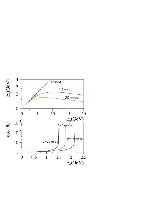
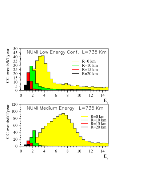
Figure 2: Top-Left – allowed $E_{\nu}$ values for several $\theta_{\nu}$ values. Bottom-Left – shows $1/\cos\theta^{*}_{\nu}$ that is proportional to the neutrino flux. $\cos\theta^{*}_{\nu}=\sqrt{1-\frac{E^{2}_{\nu}}{E^{*2}_{\nu}}\tan^{2}\theta_{\nu}}$ is the $\nu$ production angle in the rest frame of the $\pi$. Right – On and off-axis beams for the low and medium energy NuMI horns configuration. A full beam simulation was made using the Geant based GNuMI Monte Carlo.

Two toroidal magnetic horns sign and momentum-select the secondary beam. The horns are movable allowing one to obtain different neutrino energy spectra. For example, Fig. 2 depicts the expected energy spectrum at different location for the low energy (horns 10 m apart) and the medium energy (horns 27 m apart) horn configurations. As shown, the off-axis beams are characterized by having a narrow and well-defined energy distribution with fluxes higher than the corresponding on-axis energy. In addition, the harmful high energy tail (a source of NC background) of the on-axis beams is not present, as expected from energy and momentum conservation, Eq. (9). All these distributions are calculated using the GNuMI Geant based Monte Carlo [51], and include the full beamline, target and decay pipe description.

A reduction of the high energy tail of the medium energy off-axis beam is in Fig. 2. There are two reasons for this: (1) the transverse momentum of the pions is smaller for the medium energy configuration making $\Delta^{medium}_{T}<\Delta^{low}_{T}$, and (2) the mean energy of the kaons in the medium energy beam is higher producing neutrinos that are of higher energy and therefore less harmful to the analysis.

3.2.2 Anti-neutrino Fluxes

Studies of matter effects and CP violation require a comparison between $\nu_{\mu}$ and $\bar{\nu}_{\mu}$ oscillations. An anti-neutrino beam can be produced simply by reversing the polarity of the horns. This beam’s flavor composition and $(\nu_{e}+\bar{\nu}_{e})/(\nu_{\mu}+\bar{\nu}_{\mu})$ are also shown in Fig. 3. Although the $\nu_{\mu}$ contamination in the $\bar{\nu}_{\mu}$ beam is significantly larger than in the $\nu_{\mu}$ beam, the fractional $\nu_{e}+\bar{\nu}_{e}$ contamination in the $\bar{\nu}_{\mu}$ beam is roughly the same as in the $\nu_{\mu}$ beam, and in fact the ratio of the event rates in a far detector is primarily due to the difference in neutrino and anti-neutrino cross sections. At 2 GeV the cross section ratio is about 3, so to measure the same probability to equal precision in anti-neutrino running would take approximately three times longer in $\bar{\nu}$ studies. However, between matter effects and CP Violation, the $\bar{\nu}_{\mu}\to\bar{\nu}_{e}$ oscillation probability might be significantly larger than its CP conjugate, so in fact the required running time to extract physics from $\bar{\nu}$’s depends very much on what those parameters turn out to be. In later sections of this report we give sensitivities to physics parameters assuming 300 kTon Φ-years of $\bar{\nu}$ running compared to 120 kTon Φ-years of $\nu$ running, but certainly the length of time needed to see physics in $\bar{\nu}$ running depends on what the $\nu$ running has measured.

3.2.3 Systematic Uncertainties

The beamline and resulting neutrino beams described earlier in this section can (and should!) be used for both $\nu_{e}$ appearance and $\nu_{\mu}$ disappearance measurements. The two different analyses, however, depend very differently on systematic uncertainties. In this section we describe how systematic effects will contribute to the two analyses, and how the presence of both the MINOS on-axis near detector, and a possible on or off-axis near detector of the same technology as the far off-axis detector can be used.

For both measurements, however, one must be able to predict the non-oscillated $\nu_{\mu}$ spectrum to high accuracy. The MINOS experiment will have an on axis near detector which is functionally identical to the on axis far detector, and should be able to measure the $\nu_{\mu}$ event rate for the on-axis beam. As long as the observed neutrinos come from one and the same parent pion (or kaon) beam, the unoscillated $\nu_{\mu}$ spectra at two arbitrary detector locations are always strongly correlated and a measurement of one of them makes possible a prediction of the other. The technique of doing so has been shown in Ref. [52], and involves a correlation matrix: for every $\nu_{\mu}$ event at a given energy reconstructed in the near detector, there is a collection of $\nu_{\mu}$ events expected at various energies in the far detector. Because the events in the peak of both the on-axis and off-axis beams come from pion decays, the uncertainty in the $\nu_{\mu}$ flux due to hadron production alone can likely be reduced do 1-2% in the peak of the off-axis energy distribution.

An outstanding issue is the one of cross sections. With neutrino energies being significantly different in the near and far sites, uncertainties from this source will not cancel in the prediction. Ideally, precision measurements of neutrino cross sections would be required. It also possible to infer those cross sections indirectly as part of the same project, once hadron production is precisely measured.

In the absence of oscillations, one might expect roughly 15 accepted events/kTon-year between 1.5 and 2.5 GeV for an off-axis beam. So for a 100 kTon-year run, if $\theta_{23}$ really was $\pi/4$, then the statistical error on the oscillation probability could be as low as 1 to 3 divided by 1500, which is well below the 1-2% quoted above. So obviously the systematic uncertainty on the flux and the acceptance will be the dominating effect, and a near off-axis detector (combined with improved hadron production measurements, for example at E907) may improve this. Comparing the relative efficiency of an off-axis detector with the MINOS on-axis near detector to a few per cent would also be a challenge, which again would stress the need for a near detector of the same technology as the far detector.

By contrast, in an appearance search, the systematic uncertainties could actually be small compared to the uncertainty due to statistical fluctuations in the background. So, for example, if one expects roughly 0.3 intrinsic $\nu_{e}$ background events accepted per kTon year the statistical uncertainty due to the expected number of background events in a 100kTon-year experiment would be $1/\sqrt{30}$, or about 20%. Therefore, a 10% systematic uncertainty on the intrinsic $\nu_{e}$ flux would have negligible effect on the physics sensitivity. For $\nu_{e}$ background events in the signal region, most of them arise from muon decays, which in turn arise from the same parent pion decays that have been measured in the peak of the neutrino energy distribution in the MINOS near detector. The small fraction which arise from kaon decays can be constrained again by E907 measurements, and from extrapolating from higher energy $\nu_{e}$ events in the far detector.

So, while 10% uncertainties in the $\nu_{e}$/$\nu_{\mu}$ flux ratio are acceptable and even attainable using the MINOS on axis near detector, the neutral current backgrounds may prove to be far more challenging. If the neutral current background is half the size of the intrinsic $\nu_{e}$ background, then the systematic uncertainty could be twice as large (i.e. 20%) and still be negligible. On the other hand, if the neutral current background is twice the intrinsic $\nu_{e}$ background, then it needs to be known twice as well, or to 5%. There are currently large uncertainties on the neutral current cross section in the first place, so further studies (and measurements!) are needed to demonstrate how precisely one would need to know the neutral current background. These measurements would best be made in a dedicated off-axis detector of the same or more segmentation somewhere in the NUMI facility (possibly in the access shaft).

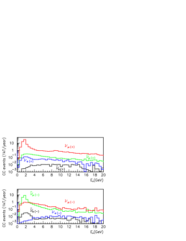
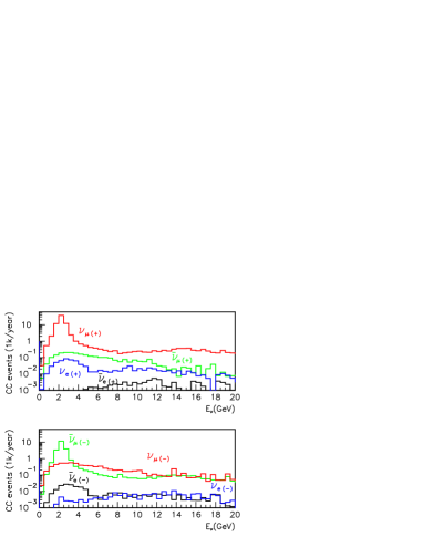
Figure 3: Beam composition for positive (+) and negative (-) horn currents. left: for the a low energy configuration at $L=735$ km and $R=10$ km. right: for the a medium energy configuration at $L=900$ km and $R=12$ km.

3.3 Potential Off-Axis Experiments

There are several possibilities for a detector for the NuMI off-axis that are being considered [53]. One can summarize the detector’s performance in this beam by two numbers, namely the efficiency for detecting a 2 GeV electron neutrino charged current event, and the efficiency for removing any neutrino interaction that is not a electron neutrino charged current event. There will be both $\nu_{\mu}$ charged current and $\nu_{\mu},\nu_{\tau}$, and $\nu_{e}$ neutral current interactions in this detector, and certainly the neutral current interactions are those which can most easily fake a $\nu_{e}$ charged current event. Of course, the physics reach for a given detector (and for a given cost) depends on those two performance numbers, as well as a cost per kTon of detector. We will first discuss the physics performance.

Since the intrinsic $\nu_{e}$ content in the NuMI off-axis beam is roughly $0.5\%$ when integrating from 1.5 to 2.5 GeV, the goal for any detector is to reduce the NC background to approximately this level. There are roughly three kinds of detectors which are being considered: fine-grained calorimetry (a absorber/readout sandwich with different options for both absorber and readout), a water cerenkov device like SuperKamiokande, and a Liquid Argon TPC, like ICARUS.

Because a liquid Argon TPC would have by far the finest segmentation and resolution, it could presumably have the highest detector efficiency and lowest background. By cutting on the dE/dx of the electron candidate track in the first radiation length, one can remove essentially all of the neutral current events, while retaining 90% of the signal [54].

Next in segmentation is the fine-grained calorimeter concept. Studies of various absorber and readout materials produce slightly different efficiencies, but roughly speaking, with a certain set of cuts, the NC events represent a background which is about half of the intrinsic $\nu_{e}$ background, while retaining roughly 40% signal efficiency [55, 56].

Finally, there is water cerenkov technology, which so far has been demonstrated in simulations (using SuperK-based phototube coverage, electronics, noise, etc.) to reduce the NC background to approximately twice the size of the intrinsic $\nu_{e}$ background, but with a signal efficiency of about 25%, because only quasi-elastic events are used in the analysis [57].

All of these studies are preliminary and work is continuing to optimize the detector responses, but for the moment one can consider in general three types of detectors: the next questions to ask are: how many kTons are needed for the three different technologies to provide comparable physics reach, and how good must the systematic uncertainty be on the background rejection? The answer depends very much on what reach one is aiming for: for a factor of 10 past the CHOOZ limit, systematics at the 20% level are acceptable, and roughly speaking, 100 kTon-NuMI-years of fine-grained calorimeter has the same reach as 25 kTon-NuMI-years of liquid argon TPC, and 400 kTon-NuMI-years of water cerenkov. This can be shown in Fig. 4. However, for a factor of 100 past the CHOOZ limit, the systematics become more important, and because of the higher background levels currently attained, Water cerenkov hits systematic limitations much sooner than the other detector technologies. It should be noted, however, that if Water Cerenkov can be shown to have better background rejection, it may remain attractive, because since only the surface need be instrumented, the cost scales like $mass^{2/3}$.

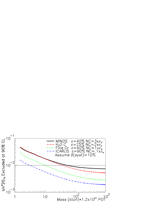
Figure 4: Expected detector performance.

While the physics performance is very different between the three, the cost/kTon is also quite different. In fact the cost/kTon is perhaps an even greater unknown than the physics performance. For example, if a 5kTon liquid argon calorimeter were to be built using 600 Ton modular structures like those used in ICARUS, the cost would be prohibitively high. If it were built using a single 7 kTon(total) module, a miniature version of the LANNDD detector [59] then it would be considerably cheaper, perhaps as low as $40$ Million dollars [59]. A 20 kTon fine-grained calorimeter has been costed as low as 30-60 Million dollars, and finally, a Water cerenkov at 80 kTon has been costed at 85 M/kTon for four water tanks [58] It is still too preliminary to make a detector choice now as these numbers as well as some of the performance numbers are quite preliminary. What is very clear between all of these detectors, however, is the fact that the cost of a Proton Driver is a far more cost-effective way to extend the physics reach, compared to increasing the detector mass. It should be noted that five times any detector cost proposed would be considerably more expensive than building a proton driver upgrade.

3.4 $\nu_{\mu}$ and $\nu_{e}$ Detector Simulation

This section presents possible analyses towards $\nu_{e}$ appearance and $\nu_{\mu}$ disappearance in a highly segmented calorimetric detector, based on simulated data. As an example, in the following studies we have assumed a detector made up of iron foils interleaved with 1 cm thick scintillator planes. The scintillator strips are oriented at plus or minus $45^{\circ}$ from vertical, alternating every other plane (two views). Detector performance was studied for different longitudinal and transverse segmentations, as well as for different spacings between two adjacent planes. Unless stated otherwise, throughout most of this section we will be assuming a longitudinal sampling every quarter of a radiation length (which in case of iron means a thickness of 4.5 mm per foil), the transverse width of each readout cell is chosen to be 2 cm, and a 3 cm long air gap is left between each two iron-scintillator pairs.

3.4.1 GMINOS Implementation

All the detector simulations were carried out with the aid of the GMINOS program, developed at Fermilab as part of the official fortran-based code for the MINOS experiment. GMINOS is a Geant-based Monte Carlo program which was widely used during the design period of the MINOS detectors. It simulates particle interactions and detector responses in a largely user-defined detector, leaving a lot of freedom for the definition of detector geometry, choice of passive and active materials and readout techniques, and of the kind of reactions under study, without the need of writing additional code or recompiling the program. The actual geometry of the detector is defined via user input cards, under the assumption of the most general modular detector structure: a repeating pattern of passive absorption planes and active detector planes oriented at some fixed angles with respect to the beam axis. Plane definition includes details of the internal structures surrounding readout cells/strips to account for the basic construction features of of fiber-scintillator, RPC and LST detectors. Each volume element is of a user-specified material and dimensions.

Neutrino interactions are generated using the NEUGEN cross sections and event generator. All hits coming from particles that deposit energy are recorded, the record contains information about particle identity, its momentum, energy loss and time-of-flight for each active volume being hit. Electronics noise and inefficiencies are included, attenuation effects in light propagation simulated and corrected for during event reconstruction.

GMINOS produces an ADAMO-structured output file, allowing a data analysis under the MAW (MINOS interface to PAW) package or a dedicated event reconstruction program; it also offers event displays in the longitudinal and face-on projections via mhpd. In Fig. 5 we show some “typical” events.

Running versions of GMINOS exist for both Linux and IRIX64 platforms. All detector optimization and performance studies herewith referred to were done by appropriate input card settings within the GMINOS framework.

3.4.2 Event Reconstruction

In a highly segmented calorimetric detector, a 1-2 GeV electromagnetic shower will leave hits in typically 10-20 consecutive planes, making possible track finding in each view. Muons of more than 0.5 GeV produce at least 40 planes long tracks; identifiable tracks, although usually shorter, are also often produced by charged pions and recoiling protons. High transverse segmentation provides good separation of two close tracks; preliminary studies in which signatures of single 1-2 GeV $\pi^{0}$’s were examined revealed that about 2/3 of them produce two separable showers in at least one view. This result is over a factor 2 better than obtained from the same study for the MINOS far detector. On the other hand, a still finer segmentation, either transverse or longitudinal, was found not leading to a significant performance improvement. In Table 2 shows the $\pi^{0}$ identification capabilities for different segmentations.

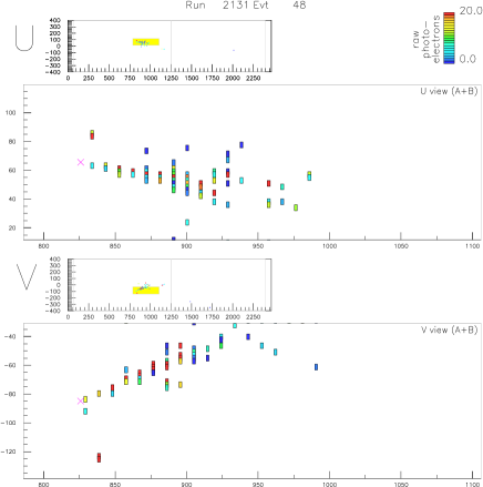
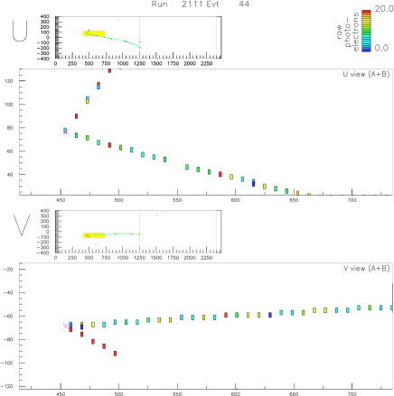
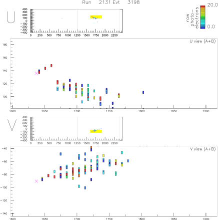
Figure 5: Typical events for $\nu_{e}$ CC, $\nu_{\mu}$ CC, and NC.

Iron	Scintillator	$\pi^{0}$ id	$e^{-}$ id
thickness	strip width	efficiency	efficiency
2.54 cm	4 cm	30%	90%
1.00 cm	2 cm	50%	90%
0.45 cm	3 cm	59%	90%
0.45 cm	2 cm	66%	90%
0.45 cm	1 cm	67%	90%
0.23 cm	2 cm	69%	90%

Table 2: $\pi^{0}$ identification capabilities for different segmentations.

Most detector optimization studies, that originally were done on a particular example of the steel and plastic scintillator design, are easily extendible to alternative designs, after defining what the equivalent segmentation is, expressed in absorber radiation lengths (longitudinally) and Molière radii (transversely). In case of a high-Z absorber, gain in performance can be obtained by including a few cm long separation (air gaps) between each two adjacent planes. This has the effect of increasing the effective mean radiation length of the detector and therefore improving the angular resolution of tracks. Dedicated simulations of the same basic steel/scintillator detector design with different air gaps revealed a steady increase of signal reconstruction efficiency as the air gaps lengths increased from 0 to 3 cm, followed by a situation where further improvement of angular resolution merely compensates the losses due to increasingly poor clustering of electromagnetic showers.

Event reconstruction is done entirely within the reconstruction program included in the GMINOS package. It consists of track fitting and applying selection criteria at both the track and the event level. Tracks are fitted and examined in each view separately. A good track is required to give hits in at least 4 planes and have good $\chi^{2}$ for a straight line. Long muon tracks, which are often not straight lines, are retrieved as being composed of two to several straight segments. Further analysis relies largely on simple track characteristics like length, width and energy.

3.4.3 $\nu_{\mu}$ CC and NC Identification

Events that fail the criteria imposed for $\nu_{e}$ appearance search, to be described in the next section, are largely dominated by NC and $\nu_{\mu}$ CC. The following simple algorithm allows a highly efficient separation of the two classes of events.

Figure 6: Efficiency for the identification of muons (top) and NC (bottom), assuming low energy beam and a 10 km off-axis detector, as a function of the track length cut value applied.

For muons of at least 0.5 GeV, the length of the produced track is to a good approximation proportional to the initial muon energy. A typical muon track is about 52 planes per view per GeV long and essentially one cell wide. In the NC events, only charged pions can produce similar tracks, but with an incident beam spectrum peaking at 2 GeV it is kinematically unlikely to have a charged pion produce a 40 planes per view long track. It is therefore sufficient to concentrate on one cell thin tracks and check for the longest track in the event to obtain two high purity samples, dominated by $\nu_{\mu}$ CC and NC, respectively. The identification efficiency for $\nu_{\mu}$ CC and for NC, depending on the actual value of the track length cut that is applied, is given in Fig. 6. For example, applying a cut at 40 planes per view, one gets a 97% overall muon identification efficiency and $>$98% efficiency for NC. The resulting samples for the medium energy beam at baseline of 900 km and a 11.5 km off-axis detector are given in Table 3.

Sample	$\nu_{\mu}$ CC	NC	$\nu_{e}$ CC
L$>$40	34.1	0.7	0.
L$<$40	1.1	39.3	2.6

	$\nu_{e}^{signal}$	$\nu_{e}^{beam}$	NC	$\nu_{\mu}$ CC
All	1.28	1.04	24.95	18.04
$\epsilon$	0.43	0.10	0.005	0.0004
Final	0.55	0.10	0.11	0.007

Table 3: Reconstruction efficiencies. LEFT: $\nu_{\mu}$ CC and NC event reconstruction as a function of the track length, L. RIGHT: for $\nu_{e}$ CC event reconstruction for energies between 1.5 to 3 GeV. We gives expected number of events for 1 kTon-year for a detector located at 11.5 km from the axis, and at a length of 900 km. $\nu_{\tau}$ CC events do not contribute because the beam energy is below the threshold of that reaction.

As is found, background in the $\nu_{\mu}$ CC sample amounts to merely 2%. The background contamination of the NC sample depends significantly on the amount of $\nu_{e}$ appearance and, as usual, we have arbitrarily assumed $|U_{e3}|^{2}=0.01$. Fig. 7 shows the muon efficiency as a function of the incident neutrino energy (top), as a function of muon energy (middle), and the NC efficiency as a function of neutrino energy (bottom), for three values of the track length cut.

Figure 7: Muon identification efficiency as a function of beam energy (top), as a function of muon energy (middle), and NC identification efficiency as a function of beam energy (bottom). Solid lines correspond to a track length cut at 40 planes per view, dashed lines to 36 planes, dotted to 32 planes.

From the track length, the muon energy can be determined to better than 10% for fully contained events. This corresponds to a similar accuracy in the beam energy measurement based on quasi-elastic events (and those inelastic events in which final state hadrons are not energetic enough to leave identifiable tracks). Extending the analysis to all events improves the statistical power by a factor 2-3, but the accuracy of neutrino energy reconstruction is limited by the uncertainty in energy measurement of hadronic and electromagnetic showers and is of $\sim$20%. Whether one or the other approach will be preferred depends mainly on the systematic uncertainties related to smearing and selection efficiency corrections that will require more detailed Monte Carlo studies, and to our knowledge of the corresponding cross sections at the time of running the experiment. Fig. 8 shows the reconstructed energy spectra of all $\nu_{\mu}$ CC for three values of $\Delta m^{2}_{23}$ and Fig. 9. the same spectra for quasi-elastic-like events only. Error bars are the statistical errors corresponding to a 20 kTon$\times$year exposure (fiducial). Clearly, from a purely statistical point of view a precise measurement of $\Delta m^{2}_{23}$ is possible.

Figure 8: Reconstructed energy distributions for all $\nu_{\mu}$ CC events for three different values of $\Delta m^{2}_{23}$. Also shown is the measured spectrum for the no oscillation case (dashed histograms) and respective ratios (lower plots).

Figure 9: Reconstructed energy distributions for quasi-elastic $\nu_{\mu}$ CC events for three different values of $\Delta m^{2}_{23}$. Also shown is the measured spectrum for the no oscillation case (dashed histograms) and respective ratios (lower plots).

3.4.4 $\nu_{e}$ CC Identification

Analysis towards $\nu_{e}$ appearance should be optimized in means of the expected “figure-of-merit”, defined as $S/{\sqrt{S+B}}$, where $S$ is the number of expected signal events under the (arbitrary) assumption of $|U_{e3}|^{2}=0.01$ and $B$ the expected residual background in the final sample per 1 kTon$\times$year.

Most tracks coming from charged pions and recoiling protons can be rejected by requiring a mean track width of at least two cells and a width at maximum of at least three cells. “Baby tracks”, that is, tracks found in the vicinity of the end of a longer main track and less than half of its length, come mostly from secondary particles within the same shower and are discarded. Conversely, two tracks of comparable length and/or pointing at the same interaction vertex are a signature of a NC event with a $\pi^{0}$ in the final state.

After track selection, a signal candidate event is required to leave exactly one good track in each view. Additional selection criteria are imposed on the event basis. To optimize the ratio of $\nu_{e}$ signal to intrinsic $\nu_{e}$ background, a window in the total visible energy is defined (for $\Delta m^{2}_{23}=0.0025-0.003$ GeV² a reasonable choice is 1-3 GeV). A small missing $p_{T}$ with respect to the beam direction is required, a minimum fraction of the total event energy carried by the track (both criteria helping reject NC), and no track longer than 28 planes in any view (suggestive of a muon). Remaining NC background is further reduced by checking for a displacement of the beginning of the shower with respect to the interaction vertex, the latter being identified by the trace of the recoiling proton (if any). The efficiency of the above criteria on generated samples of signal $\nu_{e}$ CC, background $\nu_{e}$ CC, NC and $\nu_{\mu}$ CC, is depicted in Fig. 10.

Figure 10: Initial samples per 1 kTon$\times$year for four classes of events: signal $\nu_{e}$ CC, background $\nu_{e}$ CC, NC and $\nu_{\mu}$ CC, and their reduction rates after applying subsequent selection criteria. The cuts are: 1. Visible energy, 2. One good track per view, 3. Small $p_{T}$, 4. Large energy fraction carried by track, 5. Shower starting from interaction vertex.

Figure 11: Fraction of surviving events for the four classes of events, as a function of beam energy.

The resulting reconstruction efficiency and remaining contaminations from NC and $\nu_{\mu}$ CC as a function of the incoming neutrino energy are shown in Fig. 11. To an approximation in which exactly the same analysis procedures and selection criteria are applicable, these efficiencies should be convoluted with the actual beam spectrum to obtain the overall reconstruction efficiencies and background rejection levels for any assumed beam. As is learned, for a typical NuMI off-axis beam under consideration, one gets a total signal reconstruction efficiencies of 35-42%, a rejection of about 99.7% of all NC events is obtained, while $\nu_{\mu}$ CC are suppressed to a negligible level. The total background is therefore dominated by the intrinsic $\nu_{e}$ component of the beam and any further background reduction is impractical. As an example, the total expected signal and background rates for a 10 km off-axis detector in the low energy NuMI beam per 1 kTon$\times$year are given in table.

3.5 Physics Sensitivity with $4\times 10^{20}$ Protons per year

To fully appreciate the capabilities of a Proton Driver upgrade, it is first useful to consider what physics would be available with a 20 kTon fine-grained calorimeter and a five year run, assuming $4\times 10^{20}$ protons on target per year, or the nominal NuMI intensity. The plots that follow are for a beam that is 900 km from Fermilab, and located 11.5 km perpendicular from the center of the beam.

3.5.1 $\nu_{\mu}$ Disappearance Measurements

First of all, in combination with the MINOS experiment, an off-axis experiment would dramatically improve the precision on the measurements of the atmospheric parameters, $\Delta m_{23}^{2}$ and $\theta_{23}^{2}$. As we will see in later sections, this level of precision is needed in order to be able to interpret the $\nu_{e}$ appearance data properly, and if one is to ever extract information about the CP-violating phase of the mixing matrix.

From the analysis described in section 3.4.3, we expect that for a baseline of 900km and $\Delta m^{2}_{23}$=0.002 GeV², the rate of $\nu_{\mu}$ disappearance is close to 50% and increases to 90% if $\Delta m^{2}_{23}$=0.003 GeV². In the latter case, most disfavorable from the statistical point of view, a 2% measurement of $\Delta m^{2}_{23}$ is possible after an exposure of 20 kTon$\times$years, assuming that systematics will also be under control to an appropriate level. Figure 12 depicts the measured $\nu_{\mu}$ spectra for 3 close values of $\Delta m^{2}_{23}$ near 0.003 GeV² and for two different exposures, after necessary corrections for energy smearing and selection efficiency, and the corresponding ratios between measured and predicted values. A simple fit to the latter yields a value of $\Delta m^{2}_{23}$ with a statistical error of $\pm$0.0042 GeV² for a 20 kTon$\times$year exposure and of $\pm$0.0019 GeV² for a 100 kTon$\times$year exposure. This infers a measurement to better than 2% and 1%, respectively, with purely statistical uncertainties being considered.

Figure 12: Measured $\nu_{\mu}$ energy distributions events for $\Delta m^{2}_{23}$=0.003 (solid lines), 0.00305 (dashed) and 0.0031 (dotted) GeV² after an exposure of 20 kTon$\times$years and 100 kTon$\times$years. Also shown are the respective ratios measured/predicted. Only statistical errors are considered.

3.5.2 $\nu_{e}$ Appearance Search

For the experimental parameters listed above, an off-axis experiment with a fine-grained calorimeter could expect to improve the limits on $\nu_{\mu}\to\nu_{e}$ by roughly an order of magnitude past what has already been set by the CHOOZ reactor experiment. Although Fig. 4 showed the limits one could achieve in a simple model with no matter effects and several detector options, Fig. 13 shows for the fine-grained calorimeter described above what the same plot looks like neglecting the solar mass splitting contribution, but including both possibilities of matter effects.

First, one should determine the sensitivity to observing $\nu_{e}$-appearance as a function of time (in kTon-years of detector exposure to the beam). Observing a signal depends not only on the value of $|U_{e3}|^{2}$ but also on the neutrino mass hierarchy. Fig. 13 depicts the two and three sigma sensitivity to $|U_{e3}|^{2}$ (see [55] for details) as a function of the number of kTon-years of accumulated neutrino beam data collected off-axis, in the case $\Delta m^{2}_{23}=\pm 3\times 10^{-3}$ eV², $\sin^{2}\theta_{\rm atm}=1/2$ and $\Delta m^{2}_{12}=10^{-7}$ eV², $\sin^{2}\theta_{\odot}=1/4$. First, in order to be sensitive to values of $|U_{e3}|^{2}$ which are significantly smaller than the current CHOOZ bound ($|U_{e3}|^{2}\mathrel{\mathchoice{\lower 3.0pt\vbox{\halign{$\m@th\displaystyle\hfill#\hfil$\cr<\crcr\sim\crcr}}}{\lower 3.0pt\vbox{\halign{$\m@th\textstyle\hfill#\hfil$\cr<\crcr\sim\crcr}}}{\lower 3.0pt\vbox{\halign{$\m@th\scriptstyle\hfill#\hfil$\cr<\crcr\sim\crcr}}}{\lower 3.0pt\vbox{\halign{$\m@th\scriptscriptstyle\hfill#\hfil$\cr<\crcr\sim\crcr}}}}0.05$ [60]), one is required to accumulate more than 40 kTon-years of data, in the case of a normal hierarchy, or more than 150 kTon-years in the case of an inverted hierarchy. This means, assuming the nominal NuMI beam, roughly two or eight years of running with a 20 kTon detector. Note that the $10\%$ uncertainty on the background determination dictates that, even after accumulating an infinite amount of statistics, the three sigma reach of the off axis experiment plateaus at around $|U_{e3}|^{2}\sim 1\times 10^{-3}$ ($2\times 10^{-3}$) for a normal (inverted) hierarchy. As is clear from Fig. 13, in the case of an inverted hierarchy, the sensitivity is significantly worse. This is also expected, since matter effects enhance the $\nu_{e}$ appearance rate in the case of a normal hierarchy and reduce it in the case of an inverted hierarchy.

Figure 13: Two and three sigma sensitivity reach for $|U_{e3}|^{2}$ as a function of the running time (in kTon-years), for a normal neutrino hierarchy (solid lines) and an inverted neutrino hierarchy (dashed lines). $|\Delta m^{2}_{23}|=3\times 10^{-3}$ eV², $\sin^{2}\theta_{\rm atm}=1/2$ and $\Delta m^{2}_{12}=10^{-7}$ eV², $\sin^{2}\theta_{\odot}=1/4$, $\delta=0$. For a normal neutrino mass hierarchy, a 20 kTon detector with (without) a Proton Driver upgrade will be able to exclude at a two sigma level $\nu_{\mu}\to\nu_{e}$ oscillations, if $|U_{e3}|^{2}\leq 0.00085(0.0015)$ after 5 years.

Note that the sensitivity would be significantly different for different values of $|\Delta m^{2}_{23}|$ and that, by design, the sensitivity is optimal at around $|\Delta m^{2}_{23}|\sim 3\times 10^{-3}$ eV². We have verified that it does not deteriorate significantly for $|\Delta m^{2}_{23}|\sim(2-4)\times 10^{-3}$ eV².

3.6 Physics Sensitivity with $16\times 10^{20}$ Protons per year

If there is a Proton Driver upgrade with as much as a factor of four improvement above the “nominal” proton rate, then the physics possibilities become far richer. However, in order to accurately describe just how much physics one can do, it becomes necessary to specify first what the solar mass splitting is. Simply put, if the solar mass splitting is below $10^{-5}$, then an experiment can still further the search for $\nu_{\mu}\to\nu_{e}$, and may even have the sensitivity to determine the neutrino mass hierarchy. If the solar mass splitting is higher, then signals become far more complicated, but these complications are due to the CP-violating terms, and as such are more than welcome! In this section we will outline the physics reach for three different scenarios: 1: where the solar mass splitting is too small to be measured by KamLAND, 2: where the solar mass splitting is measured at the 10% level by KamLAND, and finally 3: when the solar mass splitting is so large that KamLAND cannot accurately measure it, although it would see firm evidence for $\nu_{e}$ disappearance.

If the solar mass splitting is significantly below $10^{-4}$, then a Proton Driver upgrade would provide another factor of two in reach for $|U_{e3}|^{2}$, if $\nu_{\mu}\to\nu_{e}$ has not already been seen, as shown in Fig. 14.

3.6.1 $\Delta m^{2}_{12}\ll 10^{-5}$ eV²

If KamLAND does not observe a suppression of the reactor anti-neutrino flux, the LMA solution to the solar neutrino puzzle will be excluded [61, 62], indicating that $\Delta m^{2}_{12}\ll 10^{-5}$ eV² and/or $\tan^{2}\theta_{\odot}\ll 1$. In this case, it is well known that the CP-odd phase $\delta$ is not observable in standard long-baseline experiments, not only because solar oscillation do not have enough time to “turn on,” but also because matter effects effectively prohibit any neutrino transition governed by the solar mass-squared difference. This being the case, one can only study $\nu_{\alpha}\leftrightarrow\nu_{\beta}$ transitions governed by the atmospheric mass-squared difference.

If $\nu_{\mu}\to\nu_{e}$ has not been observed, then the additional protons will be crucial to improve the search for a non-zero $|U_{e3}|^{2}$, as shown above. However, if $\nu_{\mu}\to\nu_{e}$ has been observed at at least the three sigma level, then a Proton Driver upgrade would allow one to get statistics in anti-neutrino running in a relatively modest running time, and determine the neutrino mass hierarchy.

Consider what happens if one detects an excess of $\nu_{e}$-like events: the next step in principle would be to determine the value of $|U_{e3}|^{2}$. One can do this by performing a $\chi^{2}$ fit to the “data”. It is assumed that the atmospheric parameters $|\Delta m^{2}_{23}|=3\times 10^{-3}$ eV², $\sin^{2}\theta_{\rm atm}=1/2$ are precisely known. Fig. 14(top,right) depicts $\chi^{2}-\chi^{2}_{\rm MIN}$ as a function of $|U_{e3}|^{2}$ corresponding to 120 kTon-years of “data” collected with a neutrino beam (as defined earlier, the neutrino (anti-neutrino) beam consists predominantly of $\nu_{\mu}$ ($\bar{\nu}_{\mu}$)). Note that, while the data were simulated with $\Delta m^{2}_{23}=+3\times 10^{-3}$ eV² and $|U_{e3}|^{2}=0.008$, a different solution, with the same goodness of fit, is found for $\Delta m^{2}_{23}=-3\times 10^{-3}$ eV², $|U_{e3}|^{2}=0.015$. This implies that if the neutrino mass hierarchy is not known, instead of obtaining a precise measurement of $|U_{e3}|^{2}=0.008\pm 0.0025$ (these are two sigma error bars), one is forced to quote a less precise (very non-Gaussian) measurement: $0.0055<|U_{e3}|^{2}<0.018$ at the two-sigma confidence level.

Figure 14: top-($\chi^{2}-\chi^{2}_{\rm min}$) as a function of $|U_{e3}|^{2}$, assuming both neutrino mass hierarchies, upon analyzing simulated data consistent with $\Delta m^{2}_{23}>0$ and $|U_{e3}|^{2}=0.008$ after 120 kTon-years of neutrino-beam running (left) and 300 kTon-years of anti-neutrino-beam running (right). bottom,left-same as above, after combining the two data sets. bottom,left-difference of minimum value of $\chi^{2}$ obtained with the hypothesis $\Delta m^{2}_{23}>0$ and $\Delta m^{2}_{23}<0$ as a function of the input $|U_{e3}|^{2}$. See text for details. $|\Delta m^{2}_{23}|=3\times 10^{-3}$ eV², $\sin^{2}\theta_{\rm atm}=1/2$ and $\Delta m^{2}_{12}=10^{-7}$ eV², $\sin^{2}\theta_{\odot}=1/4$, $\delta=0$.

Fig. 14(top,right) depicts $\chi^{2}-\chi^{2}_{\rm MIN}$ as a function of $|U_{e3}|^{2}$ corresponding to 300 kTon-years of “data” collected with the anti-neutrino beam, which, assuming a 20 kTon detector and a Proton Driver improvement factor of 4, would be less than a 4 year run. As mentioned before, because of the lower cross section, anti-neutrino running produces events in a far detector with about a factor of three less statistics per proton on target. Recall that 300 kTon-years would correspond to 15 years (!) of running with the current NuMI beam configuration and a 20 kTon off-axis detector.

Again, one would have the same $\chi^{2}$ behavior as for neutrino running: but with a significant difference – this time the matter effect is reversed. The reason for this is simple: with the neutrino beam, the inverted hierarchy reduces the $\nu_{e}$ appearance signal compared to the normal hierarchy and, therefore, in order to correctly fit the data, a larger value of $|U_{e3}|^{2}$ (compared to the one obtained with the normal hierarchy) is preferred. In the case of the anti-neutrino beam, the inverted hierarchy enhances the $\bar{\nu}_{e}$ appearance signal, and a smaller value of $|U_{e3}|^{2}$ is preferred. This allows one to separate the two signs of $\Delta m^{2}_{23}$ if the information obtained with both beams is combined. This is what is done in Fig. 14(bottom, left). Note that in this case the “wrong” model is about sixteen units of $\chi^{2}$ away from the “right” model. It is also curious to note that, even with the wrong hypothesis, a similar measurement of $|U_{e3}|^{2}$ is obtained. This coincidence, which will not be considered too relevant, is a consequence of the fact that the data with the neutrino and anti-neutrino beams “pull” the measured $|U_{e3}|^{2}$ in opposite direction, and their combination meets somewhere “in the middle.”

Finally, in order to determine how well the two different signs of $\Delta m^{2}_{23}$ can be separated, Fig. 14(bottom, right) depicts $\chi^{2}_{\rm PLUS}-\chi^{2}_{\rm MINUS}$ as a function of the input value of $|U_{e3}|^{2}$, plus the input $\Delta m^{2}_{23}>0$. Note that for $|U_{e3}|^{2}\mathrel{\mathchoice{\lower 3.0pt\vbox{\halign{$\m@th\displaystyle\hfill#\hfil$\cr>\crcr\sim\crcr}}}{\lower 3.0pt\vbox{\halign{$\m@th\textstyle\hfill#\hfil$\cr>\crcr\sim\crcr}}}{\lower 3.0pt\vbox{\halign{$\m@th\scriptstyle\hfill#\hfil$\cr>\crcr\sim\crcr}}}{\lower 3.0pt\vbox{\halign{$\m@th\scriptscriptstyle\hfill#\hfil$\cr>\crcr\sim\crcr}}}}2\times 10^{-3}$, a $\chi^{2}$ separation of more than two units can be obtained. One can turn this into an exclusion of the “wrong” sign by noting that, for an average experiment, $\chi^{2}=2$ for the “correct” hierarchy, if one combines the data obtained with the two beams (2 is the number of degrees of freedom in this case). This implies that, for $|U_{e3}|^{2}=0.01$, the wrong hypothesis yields $\chi^{2}\simeq 24$, which is excluded at more than four sigma. A three sigma confidence level determination of the neutrino mass hierarchy would be obtained at $|U_{e3}|^{2}\simeq 0.005$, or a factor of 12 beyond the CHOOZ limit.

3.6.2 $10^{-4}<\Delta m^{2}_{12}<2\times 10^{-4}$ eV²

If the best fit point to the current solar data [67] is close to the true solution, the KamLAND reactor neutrino experiment will be able to not only observe a depletion of the reactor anti-neutrino flux, but also determine the values of $\Delta m^{2}_{12}$ and $\sin^{2}\theta_{\odot}$ with very good precision [61, 62, 63, 64].

This being the case, it is possible to determine $|U_{e3}|^{2}$ and $\delta$, and the mass hierarchy at the off-axis experiment. Although only one mass hierarchy is shown in the figures below, the effects due to the matter are significantly larger than those due to CP violation, and so separating the two should be possible [68].

Fig. 15 depicts the three sigma sensitivity in the ($\delta\times|U_{e3}|^{2}$)-plane for $\Delta m^{2}_{23}=3\times 10^{-3}$ eV² for 120 (300) kTon-years of running with the (anti)neutrino beam. The sensitivity depends significantly on the CP-odd phase $\delta$, and, as expected, the sensitivity is best for $\delta\sim\pi/2$ in the case of running with a neutrino beam ($\delta\sim 3\pi/2$ for the anti-neutrino beam), where the “interference” between the “CP-odd term” and the “$|U_{e3}|^{2}$ term” is constructive (i.e., one observes more events) and worse at $\delta\sim 3\pi/2$, where the “interference” is destructive. For smaller values of $\Delta m^{2}_{12}$, the ‘z-shape’ and ‘s-shape’ observed in Fig. 15 degenerate into vertical straight lines, such that the sensitivity will no longer depend on the CP-odd phase.

Figure 15: Three sigma sensitivity for observing a $\nu_{\mu}\rightarrow\nu_{e}$ signal in the $(|U_{e3}|^{2}\times\delta)$-plane, after 120 kTon-years of neutrino-beam running (black, darker line) or 300 kTon-years of anti-neutrino-beam running (red, lighter line). $\Delta m^{2}_{23}=+3\times 10^{-3}$ eV², $\sin^{2}\theta_{\rm atm}=1/2$, $\Delta m^{2}_{12}=1\times 10^{-4}$ eV², $\sin^{2}\theta_{\odot}=1/4$.

If a signal is observed, one can attempt to determine the mixing parameters $|U_{e3}|^{2}$ and $\delta$. Similar to what was done before, the atmospheric parameters $\Delta m^{2}_{23}=3\times 10^{-3}$ eV², $\sin^{2}\theta_{\rm atm}=1/2$ will be assumed known with infinite precision, and the same will now hold for the solar parameters $\Delta m^{2}_{12}=1\times 10^{-4}$ eV², $\sin^{2}\theta_{\odot}=1/4$. Furthermore, we will also assume that the neutrino mass hierarchy is known. This is done in order to not cloud the results presented here. Fig. 16(top,left) depicts the one, two, and three sigma measurement contours in the ($|U_{e3}|^{2}\times\delta$)-plane obtained after 120 kTon-years running with the neutrino beam. The simulated data are consistent with $|U_{e3}|^{2}=0.017$ and $\delta=\pi/2$. One can readily note that while $|U_{e3}|^{2}$ can be measured with reasonable precision, virtually nothing can be said about $\delta$. Furthermore, the fact that $\delta$ is not known implies that a measurement of $|U_{e3}|^{2}$ irrespective of $\delta$ is in fact less precise than what can be obtained if the solar parameters are not in the LMA region.

Figure 16: top – One, two, and three sigma measurement contours in the $(|U_{e3}|^{2}\times\delta)$-plane, after 120 kTon-years of neutrino-beam running (left) or 300 kTon-years of anti-neutrino-beam running (right). The simulated data is consistent with $|U_{e3}|^{2}=0.017$ and $\delta=\pi/2$. bottom,left – same as above, after the two data sets are combined. The solid star indicates the simulated input. bottom,right – same as before, for different simulated data points (indicated by the stars). $\Delta m^{2}_{23}=+3\times 10^{-3}$ eV², $\sin^{2}\theta_{\rm atm}=1/2$, $\Delta m^{2}_{12}=1\times 10^{-4}$ eV², $\sin^{2}\theta_{\odot}=1/4$.

In order to improve on this picture, it is imperative to prolong our “experiment” and take data with the anti-neutrino beam as well. Fig. 16(top,right) depicts the one, two, and three sigma measurement contours in the ($|U_{e3}|^{2}\times\delta$)-plane obtained after 300 kTon-years running with the anti-neutrino beam (as mentioned before, the longer running time is required in order to compensate for the “less efficient” anti-neutrino beam). Again, $|U_{e3}|^{2}$ can be measured with some precision and nothing can be said about $\delta$. A comparison of the two figures hints that a combined analyses may prove more fruitful. This is the case because while the neutrino beam yields a “z-shaped” measurement contour, the anti-neutrino beam yields an “s-shaped” contour. The reason for this is that the number of $\nu_{\mu}\rightarrow\nu_{e}$ induced events is larger for $\delta=\pi/2$ and smaller for $\delta=3\pi/2$. Therefore, the measurement will choose larger values of $|U_{e3}|^{2}$ at around $\delta=3\pi/2$ in order to compensate for this small suppression. On the other hand, the number of $\bar{\nu}_{\mu}\rightarrow\bar{\nu}_{e}$ induced events is smaller at $\delta=\pi/2$ and larger at $\delta=3\pi/2$, and the opposite phenomenon is observed.

Fig. 16(bottom,left) depicts the result of measuring $|U_{e3}|^{2}$ and $\delta$ using the combined neutrino and anti-neutrino beam “data.” The situation is significantly improved, and now, a three sigma measurement of $\delta\neq 0$ can be performed. Fig. 16(bottom,right) is similar to Fig. 16(bottom,left), except that different input values of $|U_{e3}|^{2},\delta$ are chosen. As expected, the quality of the measurement is marginally worse for $\delta=3\pi/2$ (where $\delta$ is consistent with zero at the three sigma level), and deteriorates as $|U_{e3}|^{2}$ decreases. For $\delta=\pi/2$, one cannot determine that $\delta\neq 0$ or $\pi$ (i.e., no CP-violation) at the two sigma level if $|U_{e3}|^{2}\mathrel{\mathchoice{\lower 3.0pt\vbox{\halign{$\m@th\displaystyle\hfill#\hfil$\cr<\crcr\sim\crcr}}}{\lower 3.0pt\vbox{\halign{$\m@th\textstyle\hfill#\hfil$\cr<\crcr\sim\crcr}}}{\lower 3.0pt\vbox{\halign{$\m@th\scriptstyle\hfill#\hfil$\cr<\crcr\sim\crcr}}}{\lower 3.0pt\vbox{\halign{$\m@th\scriptscriptstyle\hfill#\hfil$\cr<\crcr\sim\crcr}}}}0.004$. It should always be kept in mind that the situation deteriorates for smaller values of $\Delta m^{2}_{12}$.

3.6.3 Large $\Delta m^{2}_{12}$

If $\Delta m^{2}_{12}\mathrel{\mathchoice{\lower 3.0pt\vbox{\halign{$\m@th\displaystyle\hfill#\hfil$\cr>\crcr\sim\crcr}}}{\lower 3.0pt\vbox{\halign{$\m@th\textstyle\hfill#\hfil$\cr>\crcr\sim\crcr}}}{\lower 3.0pt\vbox{\halign{$\m@th\scriptstyle\hfill#\hfil$\cr>\crcr\sim\crcr}}}{\lower 3.0pt\vbox{\halign{$\m@th\scriptscriptstyle\hfill#\hfil$\cr>\crcr\sim\crcr}}}}2\times 10^{-4}eV^{2}$, KamLAND will not be sensitive to the very rapid oscillatory pattern, and will only be able to observe an overall suppression of the solar neutrino flux [62, 64]. In this case, the mixing angle $\sin^{2}\theta_{\odot}$ can be measured with some precision by determining the overall suppression factor, but the value of $\Delta m^{2}_{12}$ will only be constrained to be larger than some lower limit. An upper limit will be provided by future solar data. In order to be conservative, we will consider the upper bound currently provided by CHOOZ [60], and assume that $\Delta m^{2}_{\odot}\mathrel{\mathchoice{\lower 3.0pt\vbox{\halign{$\m@th\displaystyle\hfill#\hfil$\cr<\crcr\sim\crcr}}}{\lower 3.0pt\vbox{\halign{$\m@th\textstyle\hfill#\hfil$\cr<\crcr\sim\crcr}}}{\lower 3.0pt\vbox{\halign{$\m@th\scriptstyle\hfill#\hfil$\cr<\crcr\sim\crcr}}}{\lower 3.0pt\vbox{\halign{$\m@th\scriptscriptstyle\hfill#\hfil$\cr<\crcr\sim\crcr}}}}7\times 10^{-4}$ eV² for large solar angles.

If this scenario turns out to be correct, precise measurements of the atmospheric parameters and the solar mixing angle will probably be available, while $|U_{e3}|^{2}$, $\delta$ and the precise value of $\Delta m^{2}_{12}$ will remain unknown. Of course, a “short-KamLAND” or “long-CHOOZ” reactor experiment would certainly resolve this issue [65]. Such an experiment has not been proposed yet (see, however, [66]).

What are the consequences of having a very large but poorly measured $\Delta m^{2}_{12}$? The biggest consequence, perhaps, is that even for very small values of $|U_{e3}|^{2}$, a significant amount of $\nu_{e}$-like events will be observed. This implies that the “sensitivity to $|U_{e3}|^{2}$,” as discussed in the two previous sections is not a particularly meaningful quantity to study. Furthermore, as one may fear, this will also lead to a $\Delta m^{2}_{12}$ versus $|U_{e3}|^{2}$ “confusion,” (this was already alluded to in [64]) similar to the one observed between $|U_{e3}|^{2}$ and $\delta$ in the previous section (and which continues to exist here, of course). In other words, a moderate $\Delta m^{2}_{12}$ and a large $|U_{e3}|^{2}$ will yield as many events as a large $\Delta m^{2}_{12}$ and a small $|U_{e3}|^{2}$. We already learned from the previous two sections that one will be required to run both the neutrino and the anti-neutrino beams (and accumulate enough statistics with both) in order to try to disentangle the three parameters. One should keep in mind that, while the situation is rather confusing, the number of observed events is going to be large for very large values of the solar mass-squared difference.

In order to address what kind of measurement one may be able to perform under these conditions, we simulate data for $\delta=\pi/2$, $|U_{e3}|^{2}=0.012$, $\Delta m^{2}_{12}=4\times 10^{-4}$ eV², $\Delta m^{2}_{23}=3\times 10^{-3}$ eV, $\sin^{2}\theta_{\rm atm}=1/2$, and $\sin^{2}\theta_{\odot}=1/4$, assuming 120 kTon-years of neutrino beam running and 300 kTon-years of anti-neutrino beam running. As before, we assume during the data analysis that the atmospheric parameters, the neutrino mass hierarchy and the solar angle are known with infinite precision.

The results of the three parameter fit are presented in Fig. 17, where we plot the three two-dimensional projections of the three sigma surface in the ($\Delta m^{2}_{12}\times|U_{e3}|^{2}\times\delta$)-space. Many comments are in order. First of all, one should note that the solar mass difference cannot be measured with any reasonable precision – it is only slightly better known than before, namely, it lies somewhere between $2\times 10^{-4}eV^{2}$ (the KamLAND bound) and $6\times 10^{-4}$ eV² (slightly better than the CHOOZ bound). The top left-hand panel depicts the $\Delta m^{2}$ versus $|U_{e3}|^{2}$ confusion alluded to earlier quite well. It is curious to note however, that the capability to decide whether $|U_{e3}|^{2}$ is nonzero or not is not weak – the loose constraints on $\Delta m^{2}_{12}$ are already enough to guarantee that $|U_{e3}|^{2}\mathrel{\mathchoice{\lower 3.0pt\vbox{\halign{$\m@th\displaystyle\hfill#\hfil$\cr>\crcr\sim\crcr}}}{\lower 3.0pt\vbox{\halign{$\m@th\textstyle\hfill#\hfil$\cr>\crcr\sim\crcr}}}{\lower 3.0pt\vbox{\halign{$\m@th\scriptstyle\hfill#\hfil$\cr>\crcr\sim\crcr}}}{\lower 3.0pt\vbox{\halign{$\m@th\scriptscriptstyle\hfill#\hfil$\cr>\crcr\sim\crcr}}}}4\times 10^{-3}$. Most importantly, perhaps, at the three sigma level there is solid evidence that $\delta\neq 0,\pi$. The reason for this is that, for $\Delta m^{2}_{12}=4\times 10^{-4}$ and $\delta=\pi/2$, $\bar{\nu}_{\mu}\rightarrow\bar{\nu}_{e}$ transitions are very suppressed, and a zero CP-odd phase would yield far too many $\bar{\nu}_{e}$-like events when the anti-neutrino beam is on.

Figure 17: Projections of the three sigma measurement surface in the $(|U_{e3}|^{2}\times\delta\times\Delta m^{2}_{12})$-space, after 120 kTon-years of neutrino-beam running and 300 kTon-years of anti-neutrino-beam running. The simulated data is consistent with $|U_{e3}|^{2}=0.012$, $\delta=\pi/2$ and $\Delta m^{2}_{12}=4\times 10^{-4}$ eV². $\Delta m^{2}_{23}=+3\times 10^{-3}$ eV², $\sin^{2}\theta_{\rm atm}=1/2$, $\sin^{2}\theta_{\odot}=1/4$.

3.7 Physics Sensitivity vs Largest Mass Splitting

In order to conclude how much better one off-axis locations is with respect to each other requires a full evaluation of the signal and backgrounds with a realistic detector simulation and reconstruction. We have performed such analysis (Sec. 3.4.4), and we will summarize the results by evaluating a figure-of-merit (FOM) at each location for $\nu_{\mu}\to\nu_{e}$ in the case of full mixing and $|U_{e3}|^{2}=0.01$. We defined the FOM as $S/\sqrt{S+B}$, where $S$ and $B$ are the signal and background events that survive all the cuts in the reconstruction. As depicted in Fig. 18, off-axis experiments with angles between $10\leq\theta_{\nu}\leq 13$ mrad from the axis have a high FOM for all values of $\Delta m^{2}_{13}$. The high FOM is not only due to the characteristics of the beam and oscillation probabilities, but also due to the fact that in all cases we can keep the NC background at the 0.5% level, while the reconstruction efficiency is about 40%. If we look in detail at the case of $\Delta m^{2}_{13}=0.003~{}\rm eV^{2}$, we can see that the naive beam tune performed at 735 km cannot compete with smaller $\theta_{\nu}$ locations at the same baseline. This is not true for the naive beam tune performed at 900 km, where at that location $\theta_{\nu}$ is already small enough to give us a high integrated flux. We can still obtain a 20% increase in the FOM by reducing the baseline to 735 km and $\theta_{\nu}$ to 10 mrad, but at the moment this is not particularly relevant, given the current lack of knowledge of neutrino oscillations parameters.

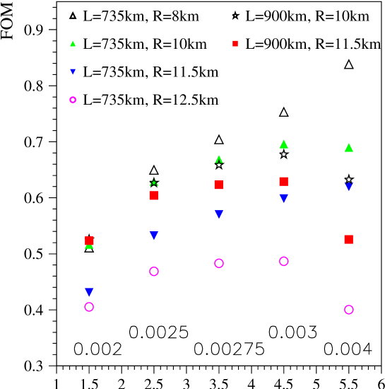
Figure 18: FOM for $\nu_{\mu}\to\nu_{e}$ appearance for different values of $\Delta m^{2}_{13}$ in the case of full mixing and $|U_{e3}|^{2}=0.01$ for different baselines and $\theta_{\nu}$, but with the same detector and reconstruction criteria. We only select events with visible energy between 1 and 3 GeV. If this highly segmented detector were at the MINOS location and $\Delta m^{2}_{13}$ were $0.003$ eV², the corresponding FOM would be 0.54. This is to be compared to the FOM for the MINOS detector that is only 0.39 [70]. This means, that if we ignore the background uncertainty, about half of the gain in sensitivity is due to the location and the other half to the detector.

3.8 Physics Reach Summary

In the presence of a Proton Driver, our ability to obtain new physics information from $\nu_{e}$ and $\bar{\nu_{e}}$ appearance depends dramatically on the solution to the solar neutrino puzzle. It should be emphasized that regardless of the outcome of the KamLAND experiment, an off-axis experiment would provide important constraints or measurements of the lepton flavor sector.

If the solution to the solar neutrino puzzle is not in the LMA region, an off-axis experiment with the current NuMI beam line is sensitive to $|U_{e3}|^{2}\mathrel{\mathchoice{\lower 3.0pt\vbox{\halign{$\m@th\displaystyle\hfill#\hfil$\cr>\crcr\sim\crcr}}}{\lower 3.0pt\vbox{\halign{$\m@th\textstyle\hfill#\hfil$\cr>\crcr\sim\crcr}}}{\lower 3.0pt\vbox{\halign{$\m@th\scriptstyle\hfill#\hfil$\cr>\crcr\sim\crcr}}}{\lower 3.0pt\vbox{\halign{$\m@th\scriptscriptstyle\hfill#\hfil$\cr>\crcr\sim\crcr}}}}0.003~{}(0.005)$ at the three sigma level for a normal (inverted) neutrino mass hierarchy. If one wishes to determine the neutrino mass hierarchy, it is necessary to also take data with an anti-neutrino beam. It should be noted that determining the neutrino mass hierarchy is not optional: the fact that the hierarchy is unknown does not permit a precise measurement of $|U_{e3}|^{2}$ even if it is sizable.

If the solution to the solar neutrino puzzle is in the LMA region and KamLAND is capable of determining the solar parameters with good precision, one can attempt to measure both $|U_{e3}|^{2}$ and the CP-odd phase $\delta$. Even if the mass hierarchy is known, measuring the CP-odd phase is not optional, as its ignorance introduces a sizable uncertainty as one tries to extract the value of $|U_{e3}|^{2}$. Again we find that combining neutrino and anti-neutrino data should provide enough information in order to discriminate maximum CP violation ($\delta=\pm\pi/2$) from no CP violation.

If the solution to the solar neutrino puzzle is in the LMA region but the solar mass-squared is not well measured (as will happen with KamLAND if $\Delta m^{2}_{12}$ is “too large”), one will be required to measure simultaneously $|U_{e3}|^{2}$, the CP-odd phase $\delta$, and $\Delta m^{2}_{12}$. Needles to say, in order to disentangle all the different contributions to $\nu_{\mu}\rightarrow\nu_{e}$ transitions, neutrino and anti-neutrino beams are required. An attempt at such a three parameter measurement is presented in Fig. 17.

In order to obtain the sensitivity and precision discussed here, many “kTon-years” of data have to be collect (especially because one is always required to run with anti-neutrinos in order to do more than just observe and excess of $\nu_{e}$-like events). This can only be achieved if 1-the neutrino flux is significantly improved with respect to the current NuMI nominal flux, 2-there is a very massive $\nu_{e}$ detector on the other end with good neutral current background rejection capabilities.

3.9 Comparison with Alternative Program to Run Concurrently

We conclude by comparing some of the results obtained here with similar studies performed for a future JHF to Kamioka neutrino beam [48]. A neutrino beam from the JHF-proton source [48] aimed at the Super-Kamiokande detector is a neutrino project with a 295 km baseline aimed to start in 2007-2008. Similar to the NuMI-off-axis project, the physics goals are to measure with an order of magnitude better precision (compared to MINOS and CNGS estimates [69]) the atmospheric parameters ($\delta(\Delta m_{\rm atm}^{2})\mathrel{\mathchoice{\lower 3.0pt\vbox{\halign{$\m@th\displaystyle\hfill#\hfil$\cr<\crcr\sim\crcr}}}{\lower 3.0pt\vbox{\halign{$\m@th\textstyle\hfill#\hfil$\cr<\crcr\sim\crcr}}}{\lower 3.0pt\vbox{\halign{$\m@th\scriptstyle\hfill#\hfil$\cr<\crcr\sim\crcr}}}{\lower 3.0pt\vbox{\halign{$\m@th\scriptscriptstyle\hfill#\hfil$\cr<\crcr\sim\crcr}}}}10^{-4}$ eV² and $\delta(\sin^{2}2\theta_{\rm atm})\mathrel{\mathchoice{\lower 3.0pt\vbox{\halign{$\m@th\displaystyle\hfill#\hfil$\cr<\crcr\sim\crcr}}}{\lower 3.0pt\vbox{\halign{$\m@th\textstyle\hfill#\hfil$\cr<\crcr\sim\crcr}}}{\lower 3.0pt\vbox{\halign{$\m@th\scriptstyle\hfill#\hfil$\cr<\crcr\sim\crcr}}}{\lower 3.0pt\vbox{\halign{$\m@th\scriptscriptstyle\hfill#\hfil$\cr<\crcr\sim\crcr}}}}0.01$), confirm $\nu_{\mu}\leftrightarrow\nu_{\tau}$-oscillations or discover sterile neutrinos by measuring the neutral current event rate, and to improve by factor of 20 the sensitivity to $\nu_{\mu}\to\nu_{e}$-appearance. After a five year program, the JHF-Kamioka program should be able to exclude, at the 90% confidence level, $\nu_{\mu}\to\nu_{e}$ transitions for $|U_{e3}|^{2}>0.0015$, while at NuMI with a 20 kTon off-axis detector we will exclude, at the two sigma confidence level, $|U_{e3}|^{2}>0.00085~{}(0.0015)$ with (without) an upgrade Proton Driver (assuming $\Delta m^{2}_{\odot}\ll 10^{-4}$ eV² and a normal neutrino mass hierarchy). The main difference between the two programs should come from the longer baseline proposed here, which allows the NuMI off-axis experiment (but not the JHF-Kamioka program) to cleanly try to address the neutrino mass hierarchy.

Underground laboratories with a Megaton detector are under discussion, but their time scale are much further away in the future.

4 Proton Economics Issues

The rate at which statistics can be accumulated in many experiments scales directly with the number of protons which can be accelerated to the appropriate energy and delivered to that experiment. This is particularly true of most neutrino oscillation experiments. For these experiments, one typically builds the largest mass of detector which meets the experimental demands and can be afforded. For world-class experiments, not only must the detector be very massive (and expensive) but the source of protons must be very intense. The Fermilab Main Injector currently provides a world-class proton facility for neutrino beams. However, even the current capabilities of the Main Injector will be stressed by the demands from the next round of neutrino oscillation experiments, and in order to keep up with the following round upgrades will be essential.

Protons accelerated in the Fermilab accelerator complex serve a variety of experimental needs. In general, the demand from multiple experiments requires that any given experiment may have fewer protons available for its specific needs than would be ideally desirable. Given that neutrino experiments can effectively use every proton which can possibly be accelerated in order to plan the broadest physics program for Fermilab one must also pay careful attention to the variety of demands which the future may bring.

In this section, we evaluate the current state of the ability of the Fermilab complex to deliver protons, extrapolate to the “near term” future experimental program (Collider, MINOS and MiniBooNE) and make some speculation regarding the longer-term future of the complex and proton economics prior to the commissioning of the new Proton Driver. In some cases, we anticipate that upgrades to the Main Injector which will also be essential for the new Proton Driver era will already start to deliver additional proton intensity even before the Proton Driver itself will be commissioned. We believe that this presents a highly attractive and sensible investment path for the laboratory.

4.1 The Current and Near-Term State of the Economy

Currently, the Main Injector is running primarily for anti-proton production for the collider. In the current mode of operation, a single batch of $\approx 4.5\times 10^{12}$ protons is first accelerated in the Booster to 8 GeV and then injected into the Main Injector and accelerated to 120 GeV before being delivered to the anti-proton production target. The current cycle for the Main Injector is 2.3 seconds. The resulting number of protons accelerated per year is about $2\times 10^{19}$, in both the Booster and Main Injector.

Starting immediately, the demand for protons accelerated in the Booster will go up dramatically with the commissioning of MiniBooNE. For MiniBooNE, six Booster acceleration cycles will be executed for every one Main Injector cycle and the resulting protons will be extracted to the MiniBooNE target. It is worth noting that the Booster would nominally be capable of delivering almost twice that number of protons except it will currently be limited due to irradiation of critical devices due to proton losses in the machine. The MiniBooNE target could certainly handle the additional protons and additional protons would be very beneficial to the experiment.

In 2005, MINOS will also begin to run and place yet more demands on both the Booster and Main Injector. MINOS requires that the Main Injector run in “Multi-Batch” mode where six bunches of protons are injected from the Booster in every MI cycle. At the same time, because of physics demand for MiniBooNE to operate in anti-neutrino mode as well as neutrino mode we anticipate that those experiments will run simultaneously placing additional demands on the Booster. We note that the nominal plan for MINOS running calls for $3.8\times 10^{20}$ protons per year delivered to the NuMI target, roughly 15 times the number of protons currently accelerated to 120 GeV. At the same time, the protons delivered for anti-proton production is also roughly planned to double from the current number for Run IIB. The number of protons which will have to be accelerated through the Booster will have to be 30 times what is currently routinely accelerated. One final consideration is that the laboratory is currently building the ability to extract Main Injector beams for test beams and experiments (one of which is already approved, E907) in the Meson area. These experiments will typically not increase the demand for protons, but affect the overall economics by requiring an extended Main Injector cycle for slow extraction.

The first step in moving towards the future has already been taken in preparations for the initial running of MiniBooNE. Upgrades to the shielding around the Booster have been added at some locations in order to ensure that external radiation limits will not reduce the number of protons which can be accelerated. In addition, beam “notching” has been introduced to reduce the exposure of critical devices to radiation upon extraction. Even with these improvements, the number of protons which can be delivered to MiniBooNE over the next year or so will be limited not by any intrinsic features of the Booster, but rather by proton losses causing the machine to become too radioactive. Work is underway to improve that situation by adding additional RF controls and strategic collimation where protons will be lost rather than in critical devices such as RF cavities. In order for MiniBooNE and MINOS to run simultaneously yet another factor of two improvement will be needed in the loss of protons compared to anything which is currently planned for MiniBooNE running.

Once MINOS begins running, the Main Injector must run in “multi-batch” mode. Currently, multi-batch mode is in a distinctly developmental status. Multi-batch operation of the Main Injector was briefly demonstrated when it was first commissioned in 1999. For that demonstration, six batches containing a total of $2\times 10^{13}$ protons were accelerated to 120 GeV. For a variety of technical reasons, it is not currently possible to replicate this operation, but with some investment in the complex it is anticipated that this should certainly be feasible again within the next year or so. In December of 2001, the study of multi-batch acceleration was once again undertaken by a group interested in studying and developing the capabilities for MINOS. The current ability to accelerate protons in multi-batch mode is limited to about $1.8\times 10^{13}$ protons per cycle. Main Injector experts believe that improvements in the RF feedback and damping will permit multi-batch operation to accelerate up to $3\times 10^{13}$ protons per batch by 2005 with one (of six) of those batches going to anti-proton production and the remaining five going to NuMI/MINOS. Note that achieving even this intensity of protons requires that the average number of protons in a Booster batch must also be $5\times 10^{12}$.

It should be noted that at present there is no defined plan that will manage to deliver all of the protons that will nominally be demanded starting in 2005. In order to even reach the “current goals” set by Beams Division a significant amount of work is required and to meet the nominal demands from the combination of Collider, MINOS, MiniBooNE and a modest test-beam program will require roughly a factor of two additional improvement beyond that. Although not yet defined, a study group has been commissioned to evaluate possible incremental improvements in the current accelerator complex which may be able to deliver this additional factor and beyond over a period of several years. In the following section, we anticipate some of the conclusions which that group will offer.

4.2 The MINOS+Collider Era, 2005 to 2008

Starting in 2005, the Fermilab accelerator complex will face an unprecedented demand for numbers of protons. In just one year, the demand for protons from the Booster and Main Injector (MI) will equal the number of protons delivered to fixed target experiments in the entire first 30 years of the laboratory. Current beams division planning assumes the following operating scenario for this era:

• Booster operation will be improved so that a total of $5\times 10^{12}$ protons will be delivered per batch.

• Main Injector operation will be improved so that a total of six batches (each with $5\times 10^{12}$ protons) can be reliably accelerated with a cycle time of 1.9 seconds.

• A total up-time of $1.8\times 10^{7}$ seconds of production acceleration cycle per year will be realized for a total of $\approx 2.8\times 10^{20}$ protons accelerated to 120 GeV per year.

• One-sixth of those protons will go to anti-proton production and five-sixths will go to the NuMI target. No significant running is currently planned (by Beams Division) for MiniBooNE running and it is assumed that running for other fixed target experiments and/or test beam will impact the total protons accelerated by no more than 10%. (This may be come in a number of different forms.)

Although the above scenario appears realistic, we note that the program is already going to be short of nominal expectations and anticipate that the following conflicts are likely to arise:

1. Under the above scenario, the number of protons delivered to the NuMI target will be only $2.5\times 10^{20}$ per year rather than the nominal design plan of $3.8\times 10^{20}$ per year.

2. A conceptual plan exists for slip-stacking one batch of protons into the Main Injector to increase the anti-proton production. The slip-stacking will increase the cycle time of the Main Injector one implemented and will cause an additional 10% reduction in the protons for NuMI.

3. No running is planned for MiniBooNE. Either a plan to accelerate more protons in the Booster by a factor of two must be developed or running MINOS and MiniBooNE simultaneously will reduce the proton intensity to the NUMI beamline by a factor of two. We anticipate that extended running of MiniBooNE is likely to be requested and recommended by the PAC.

4. Should a substantial test-beam program be undertaken one may anticipate an additional 10% reduction in protons delivered to NuMI.

Hence, we observe that in order to meet nominal demands for protons in this era, a factor of two improvement will be needed in the number of protons which can be accelerated to 8 GeV in the Booster compared to any current plan and that a factor of two improvement will also be required in the ability to accelerate protons in the Main Injector to 120 GeV from any existing plan. Furthermore, in this time-scale it is clear that these improvements will not come from commissioning of the new Proton Driver.

Fermilab and the MINOS collaboration are interested in possible modest investments which can be made in the existing accelerator complex to increase the proton intensity in this timescale. It will be particularly attractive to invest in hardware which will also be necessary in the longer term should a new Proton Driver be built. Appendix A lists possible improvements that could be made by the time NUMI starts receiving protons on their target.

The bottom line is that it appears that increasing the proton intensity within the existing accelerator complex will certainly be possible within the timescale of 2005-2008. Roughly, one might categorize the expected improvements based on level of investment and effort for a particular proton intensity. Table 4 summarizes the approximate situation that can be expected based on a particular level of investment.

Investment level	Very Rough Cost	120 GeV Protons	120 GeV Protons
		in 2005	in 2008
$\approx$None	$\approx$ $0	$1.3\times 10^{20}$	$1.3\times 10^{20}$
Small	$\approx$ $2-4 M	$2.7\times 10^{20}$	$3.0\times 10^{20}$
Medium	$\approx$ $10 M	$3.0\times 10^{20}$	$4.5\times 10^{20}$
Substantial	$\approx$ $50M	$3.5\times 10^{20}$	$9.0\times 10^{20}$
Ultimate	$\approx$ $200M	—	$16.0\times 10^{20}$

Table 4: The total protons per year which can be expected to be accelerated to 120 GeV for several different levels of investment in the existing accelerator complex. It will take time for some of the improvement programs to be carried out. Numbers are shown for 2005 and 2008 assuming an adiabatic investment. Note that these are the total protons which are accelerated, some of which go to anti-proton production, some to NuMI and a few for other purposes. Note that the investment levels all include an assumption of twice the current number of protons accelerated to 8 GeV in the Booster than currently needed just for MiniBooNE operation. MINOS expectation is $4\times 10^{20}$ protons per year. The last line gives the expectations for the most economical Proton Driver design that is available at the moment [2, 1].

4.3 2008 and Beyond; Towards the Superbeam

The physics program of Fermilab becomes less well-defined in this era. We note that the following experiments may all exist at this time with some demands for protons and/or demands on modification of the acceleration cycle from the fastest possible:

• BooNE (or other follow-on Booster neutrino experiments): Needs only Booster or new Proton Driver protons.

• CKM: Requires slow-spill extraction from the Main Injector. This has a significant impact on cycle time for experiments which do not require a slow spill. We assume that a “reasonable compromise” will be that the cycle average cycle-time reduction for anti-proton production and neutrino experiments might be about 30%.

• BTeV: Requires anti-proton production as for the current/future collider program.

• MINOS: We anticipate that regardless of a new neutrino experiment that it will be interesting to extend running of MINOS either with anti-neutrinos or for extended precision with neutrinos.

• New Off-Axis NuMI Experiment: As discussed elsewhere in this document we anticipate this to be a new important part of the Fermilab program. But it makes no additional demands on protons from MINOS!

• Test beams and other uses: We assume that these uses will be limited to no more than 10% impact on the high-rate proton production. Most likely, it can be parasitic to the impact of CKM and hence we do not include it in the impact on high-rate proton production.

Hence, the demand for protons goes up in this timescale, making relatively fewer protons available for each experiment. Using the “medium investment” estimate for proton acceleration from Table 4 we find that protons available for neutrino experiments in this era will remain below what the nominal proposal expectations set for the MINOS experiment. Specifically, the MINOS expectation is $4\times 10^{20}$ protons per year, corresponding to Main Injector power of 0.4 MW. However, the number of protons which will be delivered to the NuMI target in 2008 if all of the above conditions exist will be just $2.6\times 10^{20}$. Given that the demands for anti-neutrino running for MINOS and/or better reach in an Off-Axis detector call for yet more protons to the NuMI target, it is clear that some additional investment in proton acceleration is essential if all of these programs are to run simultaneously. We see that significant investment in the existing complex can in fact deliver more protons, but the demand from the remaining program still means that only $5.2\times 10^{20}$ protons per year can be delivered to the NuMI target. We note that this number is based on a rather large new investment in the existing accelerator complex, some of which will be attractive anyway if one anticipates a new Proton Driver. Although even more dramatic investments in the “existing” complex are possible (superbunch acceleration in both the Booster and Main Injector for instance) these start to become rather expensive and begin to be on the class of a new Proton Driver in order to go very much beyond the intensities that the “significant investment” level affords.

The ultimate beam for a Superbeam program at FNAL will require a new Proton Driver. The Proton Driver design described in [2, 1] will allow us to bring the NuMI neutrino beam power up from 0.4 MW to 1.6 MW. This design is based on an 8 GeV circular machine with a circumference of 473.2 m, and it will provide $2\times 10^{13}$ protons per pulse instead of the assumed $5\times 10^{12}$ of the current booster. In addition, the total luminosity could be further increased by 30% if the current linac gets a 200 MeV upgrade. In this case, we would get $3\times 10^{13}$ protons per pulse. This machine is estimated to cost US$160M.

An alternative design made out of only a linac to accelerate protons up to 8 GeV, using SNS and Tesla style superconducting cavities, is also under investigation [71].

In either case, changes to NuMI will be required, and are listed in appendix B, but the possibility of having a broad physics program that includes projects like NuMI and Boone running concurrently becomes realistic.

5 Conclusion

With the turn-on of the LHC in the next decade, Fermilab will relinquish its long-held position as the energy frontier in particle physics. However, given the considerable expertise that will still be resident here, and the experimental infrastructure that is currently being built, Fermilab can make a transition into being the intensity frontier of particle physics, and can take advantage of the considerable investment this field has already made in this laboratory. By upgrading the proton source that currently supplies both the collider and neutrino programs, Fermilab can not only take the next important step in neutrino flavor physics measurements, but can also extend its reach in anti-proton studies, and possibly the the host of a new cold neutron source.

While currently the most outstanding issue of neutrino flavor physics is the size of the last unmeasured mixing angle, $\theta_{13}$, seeing evidence for it is only the beginning of the story. The ultimate goals for neutrino flavor experiments are to determine the neutrino mass hierarchy, and if possible measure leptonic CP violation (assuming the solution to the solar neutrino puzzle lies in the LMA region). Both generations of experiments require a very intense neutrino beam to be able to use a long baseline, preferably with a very narrow energy spectrum to reduce the considerable backgrounds associated with these measurements. The NUMI facility which is currently being built can provide such a beam, but a new detector sensitive to $\nu_{e}$ appearance is required. To get to the second generation of experiments, namely the determination of the mass hierarchy and search for CP violation, a very intense anti-neutrino beam is required, and in order to make up for the lower anti-neutrino cross section. An upgrade of the proton source at Fermilab could be the step which finally enables us to know the number of heavy neutrinos, and ultimately whether or not there is CP violation in the lepton sector.

Appendix A Possible Strategies for Improving Proton Source in Near Term

The following is an annotated list of issues currently under discussion for possible improvements in the accelerator complex on this time scale:

1. LINAC: Upgrades to the existing LINAC offer no direct increase in intensity in the complex but some improvements could offer indirect benefits.

   • Energy increase to lower space-charge effects at injection to Booster? This could reduce proton losses and permit an extracted beam with smaller phase-space. The end result could be an increase in the total number of protons which can be accelerated in the Booster as well as better-behaved beams for stacking purposes. The cost is relatively high.

   • Chopped beam for cleaner capture in Booster: This could reduce proton losses, allowing more acceleration cycles per year. This is not a very developed concept.

2. Booster: Proton acceleration in the Booster is currently limited by unstable beam at high intensities leading to radiation from proton losses and extracted beam with poor properties for additional acceleration. Booster upgrades can both directly increase intensity and make for higher MI intensity by providing clean beams for stacking and easy acceleration. Limitations in the direct intensity increase are not completely understood but many experts estimate that it should be possible to increase intensity from the current typical operating mode, $\approx 4.5\times 10^{12}$ protons per batch, to $\approx 6-7\times 10^{12}$ protons per batch. The cost of most of these systems for the Booster are very modest compared to the cost of a new Proton Driver, but the returns are correspondingly modest.

   • Reduction in space-charge effects at injection by making longer bunches or adding electron shielding?

   • New hardware to help stabilize the beam and reduce proton losses including:

     1. Ramped correctors

     2. New RF damping hardware

     3. New collimators

     4. Larger RF cavities

     5. Inductive inserts

     6. Additional acceleration RF harmonic cavities

3. Main Injector: Improvements in the Main Injector fall into three main categories; decreasing the cycle time, improvements to permit the machine to handle more total proton flux, regardless of source, and proton stacking schemes. As the total current of protons in the machine is increased, it will be necessary to add extra RF power and damping under any circumstance, even with a new proton source. Hence, much of that investment can be viewed as “on the path” of the proton source.

   • Additional RF power to handle extra proton intensity and permit reduction in cycle time. Reduction in cycle time could be as much as 25% with no modification to existing RF cavities.

   • Reduction in cycle time by “tuning” the acceleration cycle. This probably would require very little new hardware and could result in a reduction in cycle time of 10-15%.

   • New RF damper electronics and components. This would be necessary to go to higher intensity and more sophisticated and expensive as the intensity goes even higher.

   • Inductive inserts to improve stability.

   • Collimators to protect critical components from beam losses.

   • Yet more RF power with cavity modifications and/or new cavities to reduce the ramp time even more and the total cycle time by as much as a factor of 2.

   • Slip stacking: Unlikely to be of interest for multi-batch operation.

   • Barrier RF stacking: Appears promising for increasing protons accelerated to 120 GeV by 60-70%. Requires well-behaved Booster beam and new barrier RF systems in Main Injector. Operates on principles already in use in the Recycler.

Appendix B NuMI Changes Required in Case of PD Upgrade

The NuMI Beamline is designed to handle “only” 0.4 MW of proton power, and will itself require modifications to allow it to accept five times the integrated proton power. A detailed description of the modifications required can be found in the Proton Driver machine study [4]. After a description of the beamline, we give here only a brief synopsis of those modifications. In fact, the modifications required depend very significantly on what the ultimate increase in proton power is. If one were to run NuMI with twice the proton power, the modifications would not need to be as extensive. Furthermore, several of the modifications can be avoided by changing the proton beam spot size, which although not trivial, is feasible.

The neutrino beam at NuMI is created when 120 GeV protons from the Main Injector strike a 0.94 m graphite target located roughly 40 m below ground in the NuMI tunnel. The secondary pions and kaons are then focused by two horns towards a 670 m decay pipe. The uninteracted protons and particles that did not decay hit the hadron absorber, located about 725 m from the target. Finally, beamline monitors measure the distribution of particles both upstream and downstream of the hadron absorber, and also in alcoves embedded in dolomite farther downstream. The target, the horns, and the decay pipe itself all are water cooled, and even for 0.4 MW the entire beamline requires an impressive amount of shielding due to radiation concerns.

The modifications necessary for the primary beam optics are the most trivial, assuming a cycle time at or near 1.87 seconds. Because the beamline is designed to match the dynamic aperture of the Main Injector, whatever the Main Injector supplies, the beamline can take. However, the losses per minute must be maintained at the same level as those with 0.4 MW proton power, so additional collimation may be required.

The modifications necessary for the NuMI target and horns depend critically on the spot size of the incoming proton beam. With a factor of 5 more intensity the NuMI target would be too hot after just a few pulses, with the current proton spot size. However, if both the proton beam spot size were increased by a factor of three above the current design, and the target itself was a rod three times the beam width, then the same material could withstand the increase in proton power, with similar cooling design. In fact, the current NuMI target is taller than it is wide, so it is estimated that if one had just twice the proton spot size in the vertical direction, and twice the proton power the target would not need to be upgraded. Increasing the proton spot size also means the decay pipe windows would not have to be modified from their current designs. The NuMI horns themselves suffer the most from the repeated pulsing, not from the passage of particles through them. Thus they could withstand an increase in power. However an increase in the repetition rate would change the expected horn’s lifetime. The current lifetime expectancy is 1 year, for a 1.87 second repetition rate.

The modifications for cooling the beamline are the most severe. The target area is currently cooled by a very high air flow rate. If there were 5 times the proton power the region would have to be water cooled instead. The decay pipe itself is currently being cooled by water flowing through pipes that run along its entire 670 m length. The section that would require additional cooling is less than a third of this, however. One could conceivably cut holes in the concrete shielding and add cooling pipes in that area. Finally, the hadron absorber itself would also need to be modified to allow more cooling, although the modification is not severe–the core is currently water cooled, only the first block of steel which is not cooled now would need to change. All of these upgrades require modifications to what will be highly radioactive components.

Finally, the increase in proton power will also require a new analysis of radiation safety issues. The issue of proton beam losses remaining low was addressed earlier, and if those proton beam losses are maintained, other radiation safety issues will be quite manageable. These issues are currently being addressed using extrapolations from other data, which necessarily bring in significant uncertainties, which translate into large safety factors. It is expected that the measurements of the water pumped from the NuMI tunnel and released to the surface waters will be greater than a factor of ten below the surface water limits. Similarly it is expected that measurements from NuMI’s monitoring wells will be negligible. Extrapolating from these measurements would show an upgrade in a factor of 4 in intensity to be feasible. As for airborne activation, it is likely that the target shielding and hadron absorber will need additional air seals, but given the new cooling that will also be required, this would be a minor additional cost.

In summary, the most significant upgrades required in the NuMI beamline would be those associated with cooling and sealing the target hall, and a new target with cooling. The decay pipe and absorber cooling would be the next most costly changes. Radiation safety issues do not drive any of the costs. The overall cost for a NUMI upgrade to accept 4 times the intensity and a 1.5 second repetition rate would range between 4 and 16 million dollars, which, although substantial, is less than 10 % of the cost of a new proton source.

References

- [1] “The Proton Driver Design Study”, W. Chou editor, FERMILAB-TM-2136 (December, 2000).
- [2] “Physics Study Group Report On Physics Potential at FNAL with Stronger Proton Sources”, C. Ankenbrandt et al., http://projects.fnal.gov/protondriver.
- [3] http://www-bd.fnal.gov/icfa/workshops/20/.
- [4] G.W. Foster, W. Chou, E. Malamud, et al.,, Fermilab-TM-2169.
- [5] G.Barenboim et al.,, hep-ph/0108199; G.Barenboim, L.Borissov and J.Lykken, hep-ph/0201080.
- [6] LSND Coll. (C. Athanassopoulos et al.), Phys. Rev. Lett. 75, 2650 (1995); 77, 3082 (1996); 81, 1774 (1998); W.C. Louis for the LSND Coll., Nucl. Phys. B (Proc. Suppl.) 91, 198 (2001); LSND Coll. (A. Aguilar et al.), hep-ex/0104049.
- [7] A.O. Bazarko for the MiniBooNE Coll., Nucl. Phys. B (Proc. Suppl.) 91, 210 (2001), http://www-boone.fnal.gov/.
- [8] J. Carpenter et al., Physica B270 (1999) 272.
- [9] “Scientific Opportunities with Advanced Facilities for Neutron Scattering,” Shelter Island Workshop, October 23-26, 1984, BNL Report No. Conf-84-10256.
- [10] “The Investigation of Fundamental Interactions with Cold Neutrons,” Ed. G. L Greene, NBS Special Pub. No. 711 (February, 1986).
- [11] “Proc. of the International Workshop on Particle Physics with Slow Neutrons,” Eds. O. Zimmer, J. Butterworth, V. Nesvizhevsky, and E. Korobkina, ILL France, October 22- 24, 1998, Nucl. Inst. and Meth. A440 (2000) 471.
- [12] I.B. Khriplovich and S.K. Lamoreaux, “CP Violation Without Strangeness”, Springer (1997).
- [13] P. G. Harris et al., Phys. Rev. Lett. 82 (1999) 904.
- [14] R. Golub and S. K. Lamoreaux, Phys. Reps. 237 (1994) 1.
- [15] T. Dombeck et al., Argonne Laboratory Rep. PHY-9814-TH-2001 (March, 2001).
- [16] The experiment is described in R. Huffman et al., Nature 403 (2000) 62.
- [17] T. Dombeck et al., submitted to Phys. Rev. A; M. Schuster et al., Z. Phys. B85 (1991) 49; and E. Jericha et al., Nucl. Inst. and Meth. A379 (1996) 330.
- [18] Super-Kamiokande Coll. (Y. Fukuda et al.), Phys. Rev. Lett. 81, 1562 (1998).
- [19] NUSEX Coll. (M. Aglietta et al.), Europhys. Lett., 8, 611 (1989); R. Becker-Szendy et al., Phys. Rev. D46, 3720 (1992); Kamiokande Coll. (Y. Hirata et al.), Phys. Lett. B280, 146 (1992); Kamiokande Coll. (Y. Fukuda et al.), Phys. Lett. B335, 237 (1994); Frejus Coll. (K. Daum et al.), Z. Phys. C66, 417 (1995); W.A. Mann, for the Soudan 2 Coll., Nucl. Phys. B (Proc. Suppl.) 91, 134 (2001); B.C. Barish, for the MACRO Coll., Nucl. Phys. B (Proc. Suppl.) 91, 141 (2001).
- [20] Homestake Coll. (B.T. Cleveland et al.), Astrophys. J. 496, 505 (1998); GALLEX Coll. (W. Hampel et al.), Phys. Lett. B447, 127 (1999); Y. Suzuki, for the Super-Kamiokande Coll., Nucl. Phys. B (Proc. Suppl.) 91, 29 (2001); V.N. Gavrin, for the SAGE Coll., Nucl. Phys. B (Proc. Suppl.) 91, 36 (2001); E. Bellotti, for the GNO Coll., Nucl. Phys. B (Proc. Suppl.) 91, 44 (2001); Super-Kamiokande Coll. (S. Fukuda et al.), hep-ex/0103032.
- [21] SNO Coll. (Q. R. Ahmad et al.), Phys. Rev. Lett. 87, 071301 (2001).
- [22] SNO Coll. (Q. R. Ahmad et al.), nucl-ex/0204008.
- [23] J.N. Bahcall, M.H. Pinsonneault, and S. Basu, astro-ph/0010346.
- [24] see, for example, J.W.F. Valle, Phys. Lett. B199, 432 (1987); E. Akhmedov, Phys. Lett. B213, 64 (1988); C.S. Lim and W. Marciano, Phys. Rev. D37, 1368 (1988); M. Gasperini, Phys. Rev. D38, 2635 (1988); M.M. Guzo, A. Masiero, ansd S.T. Petcov, Phys. Lett. B260, 154 (1991); S. Coleman and S.L. Glashow, Phys. Lett. B405, 249 (1997); S.L. Glashow et al., Phys. Rev. D56, 2433 (1997); G.L. Fogli et al., Phys. Rev. D59, 117303 (1999); P. Lipari and M. Lusignoli, Phys. Rev. D60, 013003 (1999); M.C. Gonzalez-Garcia et al., Phys. Rev. Lett. 82, 3202 (1999); V. Barger et al., Phys. Lett. B462, 109 (1999); J. Pulido and E. Akhmedov, Phys. Lett. B485, 178 (2000); E. Lisi, A. Marrone, and D. Montanino, Phys. Rev. Lett. 85, 1166 (2000); S. Bergmann et al., Phys. Rev. D62, 073001 (2000); O. Miranda et al., Nucl. Phys. B595, 360 (2001); D. Majumdar, A. Raychaudhuri, and A. Sil, Phys. Rev. D63, 073014 (2001); M.M. Guzzo, H. Nunokawa, and R. Tomàs, hep-ph/0104054.
- [25] B. Achkar et al., Nucl. Phys. B434, 503 (1995); CHOOZ Coll. (M. Apollonio et al.), Phys. Lett. B466, 415 (1999); Palo Verde Coll. (F. Boehm et al.), Nucl. Phys. (Proc. Suppl.) 77, 166 (1999).
- [26] CCFR Coll. (A. Romosan et al.), Phys. Rev. Lett. 78, 2912 (1997); L. Ludovici for the CHORUS Coll., Nucl. Phys. B (Proc. Suppl.) 91, 177 (2001); M. Mezzeto for the NOMAD Coll., Nucl. Phys. B (Proc. Suppl.) 91, 184 (2001); K. Eitel for the KARMEN Coll., Nucl. Phys. B (Proc. Suppl.) 91, 191 (2001).
- [27] A.M. Gago et al. Phys. Rev. D 64, 073003 (2001); M.C. Gonzalez-Garcia et al. Phys. Rev. D 64, 096006 (2001); P. Huber and J.W.F. Valle, Phys. Lett. B523, 151 (2001) and references within.
- [28] SNO Coll. (Q.R. Ahmad et al.), nucl-ex/0204009; V. Barger et al., hep-ph/0204253; P. Creminelli, G. Signorelli, and A. Strumia, JHEP 0105, 052 (2001) [see hep-ph/0102234 for update including the SNO data]; A. Bandyopadhyay et al., hep-ph/0204286; J.N. Bahcall, M.C. Gonzalez-Garcia, and C. Peña-Garay, hep-ph/0204314; P. Aliani et al., hep-ph/0205053; and many references within.
- [29] N. Fornengo, M.C. Gonzalez-Garcia, and J.W.F. Valle, Nucl. Phys. B580, 58 (2000) and references therein.
- [30] G.L. Fogli et al., Nucl. Phys. B (Proc. Suppl.) 91, 167 (2001); A. De Rújula, M.B. Gavela and P. Hernández, Phys. Rev. D63, 033001 (2001); G. L. Fogli, E. Lisi, and A. Marrone, Phys. Rev. D 64, 093005 (2001).
- [31] G. L. Fogli, E. Lisi and A. Marrone, Phys. Rev. D 64, 093005 (2001).
- [32] K2K Coll. (S.H. Ahn et al.), Phys. Lett. B511, 178 (2001); K. Nakamura for the K2K Coll., Nucl. Phys. B (Proc. Suppl.) 91, 203 (2001); J.E. Hill for the K2K Coll., hep-ex/0110034.
- [33] S.G.. Wojcicki for the MINOS Coll., Nucl. Phys. B (Proc. Suppl.) 91, 216 (2001), http://www.hep.anl.gov/ndk/hypertext/minos_tdr.html.
- [34] A. Rubbia, Nucl. Phys. B (Proc. Suppl.) 91, 223 (2001), http://proj-cngs.web.cern.ch/proj-cngs/cngs.htm .
- [35] A. Piepke for the KamLAND Coll. Nucl. Phys. B (Proc. Suppl.) 91, 99 (2001).
- [36] R. Barbieri and A. Strumia in [28]; V. Barger, D. Marfatia, and B. Wood, Phys. Lett. B498, 53 (2001); H. Murayama and A. Pierce, hep-ph/0012075.
- [37] A. de Gouvêa and C. Peña-Garay, Phys. Rev. D 64 113011 (2001).
- [38] A. Strumia and F. Vissani, JHEP 0111, 048 (2001).
- [39] S. A. Dazeley for the KamLAND Coll., arXiv:hep-ex/0205041.
- [40] A. de Gouvêa, A. Friedland, and H. Murayama, JHEP 0103, 009 (2001).
- [41] G. Ranucci et al., Nucl. Phys. B (Proc. Suppl.) 91, 50 (2001).
- [42] A. de Gouvêa, A. Friedland, and H. Murayama, Phys. Rev. D60, 093011 (1999).
- [43] see, for example, M.C. Gonzalez-Garcia, C. Peña-Garay, and A.Yu. Smirnov, Phys. Rev. D63, 113004 (2001); V. Barger, D. Marfatia and K. Whisnant, Phys. Rev. D 64, 073009 (2001).
- [44] see, for example, G.L. Fogli, E. Lisi, and D. Montanino, Phys. Lett. B434, 333 (1998); D. Majumdar and A. Raychaudhuri, Pramana 52, L529 (1999); F.L. Villante, G. Fiorentini and E. Lisi, Phys. Rev. D59, 013006 (1999); J.N. Bahcall, P.I. Krastev, and A.Yu. Smirnov, Phys. Lett. B477, 401 (2000); Phys. Rev. D62, 093004 (2000); D63, 053012 (2001); M. Maris and S.T. Petcov, Phys. Rev. D62, 093006 (2000); G.L. Fogli et al., hep-ph/0102288; V. Barger, D. Marfatia and K. Whisnant, hep-ph/0104166.
- [45] see, for example, H. Minakata and H. Nunokawa, Phys. Lett. B 504, 301 (2001); C. Lunardini and A.Yu. Smirnov, hep-ph/0106149; M. Kachelriess et al., hep-ph/0108100; and many references therein.
- [46] see H. Ejiri, Nucl. Phys. B (Proc. Suppl.) 91, 255 (2001), and references therein for the current data; see, for example, E. Fiorini, Nucl. Phys. B (Proc. Suppl.) 91, 262 (2001), for future prospects.
- [47] H.V. Klapdor-Kleingrothaus, H. Pas, and A.Yu. Smirnov, Phys. Rev. D63, 073005 (2001); A. Wodecki and W.A. Kaminski, Int. J. Mod. Phys. A15, 2447 (2000); K. Matsuda, N. Takeda, and T. Fukuyama, hep-ph/0012357 S.M. Bilenky, S. Pascoli, and S.T. Petcov, hep-ph/0102265; hep-ph/0104218; and references therein.
- [48] Y. Itow et al., hep-ex/0106019, KEK-REPORT-2001-4, ICRR-REPORT-477-2001-7, TRI-PP-01-05, Jun 2001.
- [49] P. Antonioli for the MONOLITH Coll., Nucl. Phys. (Proc. Suppl.) 100, 142 (2001).
- [50] J. Hylen et al. “Conceptual Design for the Technical Components of the Neutrino Beam for the Main Injector (NuMI),” Fermilab-TM-2018, Sept., 1997.
- [51] http://www.hep.harvard.edu/m̃essier/gnumi.
- [52] A. Para, M.Szleper, NuMI-B-781.
-
[53]
Letter Of Intent,
http://www-numi.fnal.gov/fnal_minos/new_initiatives/new_initiatives.html. - [54] ICARUS Coll., F. Arneodo, et al., hep-ph/0103008.
- [55] G. Barenboim, A. de Gouvêa, M. Szleper and M. Velasco, hep-ph/0204208.
- [56] M.Szleper, http://www-numi.fnal.gov/fnal_minos/new_initiatives/new_initiatives.html.
- [57] M. Messier, http://www-numi.fnal.gov/fnal_minos/new_initiatives/new_initiatives.html.
- [58] M. Diwan, provate communication.
- [59] D. Cline, http://www-numi.fnal.gov/fnal_minos/new_initiatives/new_initiatives.html.
- [60] CHOOZ Coll. (M. Apollonio et al.), Phys. Lett. B466, 415 (1999).
- [61] See, for example, talk by K. Ishihara at the NuFact’01 Workshop, May 24–30, 2001, Tsukuba, Japan. Transparencies can be found at http://psux1.kek.jp/ nufact01/.
- [62] A. de Gouvêa and C. Peña-Garay, Phys. Rev. D 64, 113011 (2001).
- [63] V. D. Barger, D. Marfatia and B. P. Wood, Phys. Lett. B498, 53 (2001); H. Murayama and A. Pierce, Phys. Rev. D 65, 013012 (2002).
- [64] R. Barbieri and A. Strumia, JHEP 0012, 016 (2000).
- [65] This was first mentioned in A. Strumia and F. Vissani, JHEP 0111, 048 (2001), and further explored in S. T. Petcov and M. Piai, hep-ph/0112074.
- [66] S. Schoenert, T. Lasserre and L. Oberauer, hep-ex/0203013.
- [67] G.L. Fogli et al., hep-ph/0106247; A. Bandyopadhyay et al., hep-ph/0106264; P. Creminelli, G. Signorelli, and A. Strumia, hep-ph/0102234 – updated version (July 2001); P.I. Krastev and A.Yu. Smirnov, hep-ph/0108177.
- [68] H. Minakata and H. Nunokawa hep-ph/0111131 published in Nucl. Phys. Proc. Suppl. 110 404 (2002).
- [69] V.D.Barger et al., Phys. Rev. D 65,053016 (2002).
- [70] M. Diwan, M. Messier, B. Viren, L. Wai,“A study of sensitivity in MINOS”, NuMI-NOTE-SIM-0714.
- [71] http://tdserver1.fnal.gov/foster.