JLC Overview

Abstract

JLC is an $e^{+}e^{-}$ linear collider designed for experiments at $\sqrt{s}=500$ GeV with a luminosity of up to about $2.5\times 10^{34}/cm^{2}/s$. In this talk, after describing the parameters of JLC accelerator and detector, the feasibilities of JLC to study Higgs, Top, and SUSY physics are presented based on the ACFA report.

1 Introduction

JLC is a linear collider for $e^{+}e^{-}$ collision at the energy frontier. The designed initial center-of-mass energy of the collider is 500 GeV with a luminosity of up to about $2.5\times 10^{-34}/cm^{2}/s$. In this energy region, the production of a light Higgs boson is expected, in addition to the high statics productions of Top quarks and $W$ bosons. The productions of other new particles are also predicted in models such as SUSY models. Studies of these particles at JLC will make an indispensable contribution to our understanding of the fundamental forces and constituents.

Considering the importance of the $e^{+}e^{-}$ linear collider project, the Asian Committee for future Accelerators (ACFA) has initiated a working group to study physics scenarios and experimental feasibilities at the linear collider in 1997[1]. Four ACFA workshops have been held since then, and the group published a report in summer 2001[2]. This report consists of discussions on physics at JLC, studies of a detector for JLC, and optional experiments using $\gamma-\gamma$, $\gamma-e^{-}$, and $e^{-}e^{-}$ collisions. Since it is impossible to cover everything in a short time, selected topics from the report are presented in this talk.

In the following two sections, the parameters of the JLC accelerator and the detector are described. In the subsequent section, selected topics concerning the physics on Higgs, Top and SUSY are described. Please see the ACFA report[2], for topics not covered here.

2 Accelerator

The layout of the JLC accelerator is shown in Fig. 1. The accelerator consists of two systems: one for electrons and the other for positrons. In the electron system, electrons are generated by an $e^{-}$ gun and accelerated to about 2 GeV by the Linac; the emittance is reduced by the damping ring (DR) and the longitudinal beam size is reduced by the bunch compressors (BC1, BC2). The electrons are then accelerated to by the Pre-Linac (up to 10 GeV), and then by the Main Linac. The final focus system (FFS) focuses the beam size at the interaction points (IP). The positron system is similar to the electron one, except for positron generation. Positrons are generated by injecting high energy electrons on a high Z target. For efficient collection of the produced positrons, an additional dumping ring (Pre-DR) is inserted before DR.

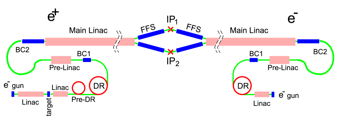
Figure 1: JLC Accelerator layout.

The parameters of the JLC accelerator are summarized in Table 1. The first three columns (A, X, Y) are parameters described in the ACFA Report[2]. The A is a typical parameter set which we can expect at the early stage of accelerator operation. Together with the operation, tuning of the machine is proceed, and we will be able to operate high current beams with very low emittances, and the luminosity as high as the Y parameter can be expected. Recently, the international Technical Review Committee has been organized to review accelerator technology developed in each region. The last two columns in Table 1 show the parameters prepared for that committee. The TRC-500 parameter is similar to the Y parameter as for as the luminosity is concerned.

Table 1: Parameters of the JLC accelerator. ^†) ACFA Report 2001, ^‡) Technical Review Committee JLC/NLC(X)[3]. TRC(C) is in preparation .

		A†)	X†)	Y†)	TRC(X)‡)
Center-of-mass energy	GeV	535	497	501	500	1000
Repetition rate	$Hz$	150				100
Luminosity	$10^{33}/cm^{2}s$	9.84	15.48	27.0	25.0	25.0
Nominal luminosity	$10^{33}/cm^{2}s$	6.82	11.15	18.20	15.2	15.7
Integrated luminosity/year($10^{7}s$)	$fb^{-1}$	98	155	270	250	250
Bunch separation	$nsec$	2.8	1.4
Bunch charge	$10^{10}$	0.75	0.55	0.70	0.75
Loaded gradient	$MV/m$	59.7	54.2	50.2	55
No. of bunches/pulse		95	190		192
Linac length/beam	$km$	5.06		5.50	6.3	12.9
AC power (2 linacs)	$MW$	118		128	150	200
Bunch length	$\mu m$	90		80	110
Emittance at IP ($\gamma\epsilon_{x}/\gamma\epsilon_{y}$)	$10^{-8}m$-$rad$	400/6.0	400/4.0		360/40
Beta function at IP($\beta_{x}/\beta_{y}$)	$mm$	10/0.10	7/0.08		8/0.11	13/0.11
Beam size at IP($\sigma_{x}/\sigma_{y}$)	$\mu m$	277/3.39	239/2.57	239/2.55	243/3.0	219/2.3
Beamstrahlung energy loss ($\delta_{B}$)	%	4.42	3.49	5.22	4.7	8.9
No. of photons per $e^{-}/e^{+}$		1.10	0.941	1.19	1.3	1.3

From an experimental point of view, the JLC accelerator has several unique features. Firstly, the JLC beam has a special time structure. One pulse of the JLC beam consists of many bunches with a small time separation of 2.8 nsec to 1.4 nsec. The pulse length of the beam is about 270 nsec, while there is a very long interval on the order of 10 msec between each pulse. This makes it hard to make an event trigger during a beam pulse while leaving sufficient time for a trigger decision between the pulses.

Secondly, due to the magnetic field produced by the opposite beam of high charge density, beam particles loose their energy and emit low energy $e^{\pm}$ and $\gamma$ particles, which is known as Beamstrahlung. The beamstrahlung smears the collision energies and reduces the effective luminosity at the nominal center-of-mass energy. The amount of this effect depends on the accelerator parameters, and it becomes significant just above the threshold of particle production where the production cross section changes rapidly with the energy. The spectra in the case of A and Y parameters are shown in Fig. 4 together with the bremsstrahlung spectra.

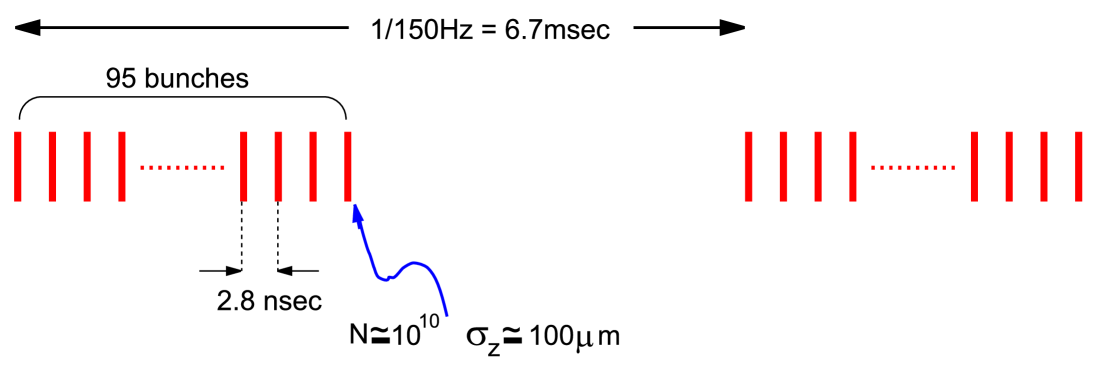
Figure 2: Structure of the JLC beam pulse.

       

Figure 3: Bremsstrahlung and beamstrahlung spectrum.

Figure 4: Example of the beam energy spread at 250 GeV for various RF phase combinations.

Thirdly, the energy spread of the beam in the main linac is relatively larger than that of conventional circular colliders, since there are no strong bending magnets to fix the energy. However, the spread of the collision energy can be controlled to some extent by adjusting the RF phases of the linacs. We will be able to select the spectrum such as a wide but short tail spectrum, or a narrow but long tail spectrum, depending on the physics requirements. The typical spectrum is shown in Fig. 4.

Lastly, if bypass lines along the main linac are prepared, we can take data at lower energies without significant changes to the facility. A run at the $Z_{0}$ pole is useful for detector calibration. The cross sections of $W$ pair production and top quark production are maximum at their threshold. The same is true for the production of the light Higgs boson. Since the energies for them are different, possibility to conduct experiments at different energies is important to maximize the physics output of the JLC.

3 Detector

The goals of the JLC detector performance have been set as follows:

• Efficient, high-purity $b/c$ tagging capability.

• A momentum resolution of the tracking devices sufficiently good so that the missing mass measured in the process $e^{+}e^{-}\rightarrow ZH\rightarrow\ell\bar{\ell}X$ is only limited by the spread of the initial beam energy.

• The resolution of the calorimeter is good enough so that the invariant mass of a 2 jets system is comparable with that of the natural width of $W$ and $Z$.

• Good hermeticity so that invisible particles can be identified efficiently.

• Beam related backgrounds must be shielded by the masking system completely. The detector must be equipped with a time-stamping device so as to identify the bunch of the event and to reduce the backgrounds which come from different bunches, but in the same beam pulse.

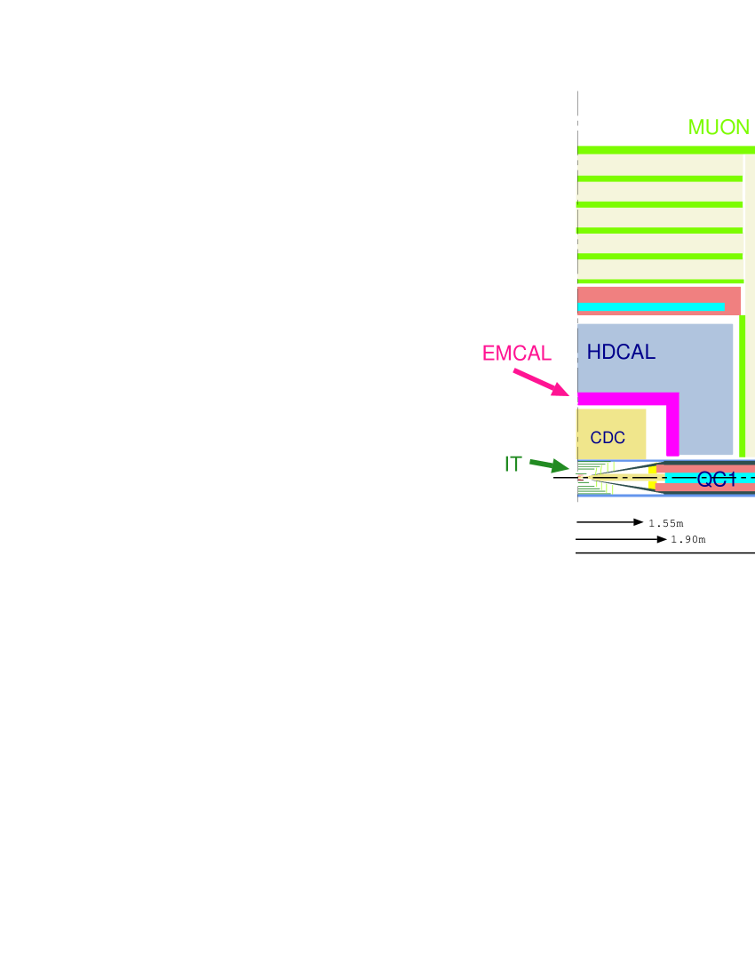
Figure 5: Cross section of the JLC detector.

To this end, a general purpose detector was considered as a basis for physics studies and the development of detector technologies. A cross-sectional view of the detector is shown in Fig. 5, and the detector system near the interaction region is shown in Fig. 6. All of the detectors except for the muon detector are placed inside a solenoidal magnetic field of 3 Tesla. With a sandwiched lead-scintillator system, the calorimeter is aimed to achieve a resolution of $15\%/\sqrt{E}({\rm GeV})\oplus 1\%$ for electro-magnetic particles and $40\%\sqrt{E}({\rm GeV})\oplus 2\%$ for hadronic particles. A central tracking device is a small cell jet chamber. Together with a CCD vertex detector, a momentum resolution($\frac{\sigma_{p_{t}}}{p_{t}}$) of $1\times 10^{-4}p_{t}({\rm GeV})\oplus 0.1\%$ is expected. In the forward region, the region above 200 mrad is fully covered by the calorimeter. For the region below 200 mrad, an active mask, a luminosity monitor and a pair monitor will be used to measure energetic $e^{+}/e^{-}$; thus, the minimum veto angle is 11 mrad. Please see the ACFA report[2] concerning detector hardware studies performed to achieve these design goals.

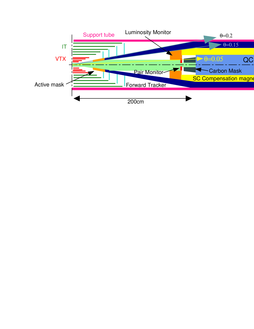
Figure 6: The JLC detector system near IP

4 Physics

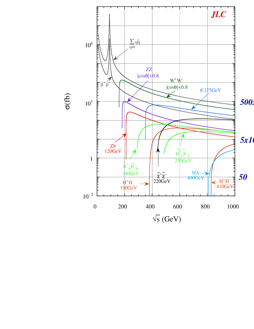
Figure 7: Cross sections of standard model processes and new particle productions. The number of events corresponding to an integrated luminosity of 500 $fb^{-1}$ is indicated on the right.

The total cross sections of the standard model processes and new particle productions are shown in Fig. 7. With the machine parameters of Y in Table 1, we can expect to collect data of the integrated luminosity of 500 fb^-1 within two years. This will allow us not only discoveries of new particles but also precise studies of new particles and the standard model particles. The expected precisions that we can obtain from these studies and the implications for physics beyond the standard model are described in the ACFA report in detail. Here, selected topics on Higgs, Top and SUSY physics are described in the following subsections.

4.1 Higgs

The standard model of elementary particles consists of three families of matter fermions, gauge bosons and Higgs boson. Gauge bosons are massless due to gauge symmetry, but they acquire masses when Higgs spontaneously breaks the symmetry. Though the gauge nature of forces among fermions has been tested very precisely experimentally[5], the key feature of the standard model, that the symmetry is broken by the Higgs, has yet to be confirmed experimentally. To this end, first of all, the Higgs particle must be discovered.

In the standard model, the mass of the Higgs boson is just a parameter. However, its self energy diverges with its mass. It is so divergent that if its mass is heavier than about 200 GeV, new physics must show up below the GUT energy and GUT models must be abondened. If it is light, the Higgs can be elementary up to the GUT energy.

Figure 8: Feynman diagram of Higgs production at JLC; (a) Higgs-strahlung, (b) $WW$ fusion, (c) $ZZ$ fusion

Although the Higgs boson has been searched extensively, no signal of direct production has been found, and a lower mass bound of 114.1 GeV at the 95% confidence level has been set[4]. On the other hand, the precise measurements of the standard model processes allow us to probe tiny loop effects of the Higgs boson. According to a global analysis of the electro-weak data, the most probable value of the Higgs boson mass is $106^{+57}_{-38}$ GeV while it is less than 222 GeV at the 95% CL[5]. Thus the Higgs boson is likely to be light and its production is expected at an early stage of the JLC experiments.

Feynman diagrams of the Higgs production at JLC are shown in Fig. 8. They consists of Higgs-strahlung from $s$-channel $Z$ boson, and $t$-channel productions by $WW$ and $ZZ$ fusion. The total cross sections of the Higgs production near to the threshold region are shown in Fig. 9. For a Higgs of mass 120 GeV, the cross section is maximum at a center-of-mass energy of about 250 GeV. For this case, its production is mainly by the Higgs-strahlung process, while at 500 GeV, about half of the cross section is due to the $WW$ and $ZZ$ fusion processes.

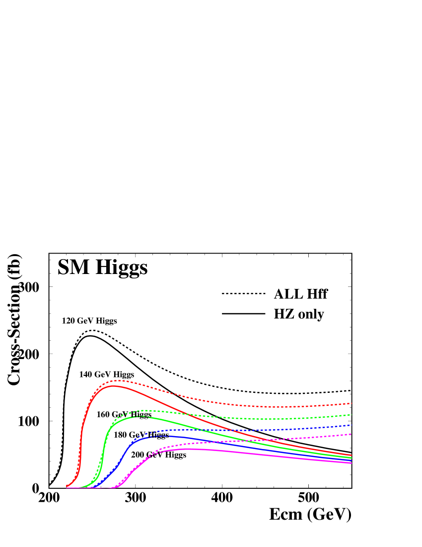
Figure 9: Total cross section of Higgs production at the JLC energy region, for Higgs masses of 120, 140, 160, 180, and 200 GeV. The cross sections of the Higgs-strahlung process are indicated by the solid lines, while those of all diagrams are shown by the dotted lines.

As an example of the Higgs study at JLC, we consider an experiment at $\sqrt{s}$=250 GeV and a Higgs mass of 120 GeV. For this case, the Higgs is produced mainly by Higgs-strahlung and it decays mainly to $b\bar{b}$ (Branching ratio of $H\rightarrow b\bar{b}$ decay is about 67%). Therefore the event signature of Higgs production is categorized, according to the decay mode of $Z$, to 4 jets, 2 jets + missing, or 2 jets + 2 leptons as shown in Fig. 10.

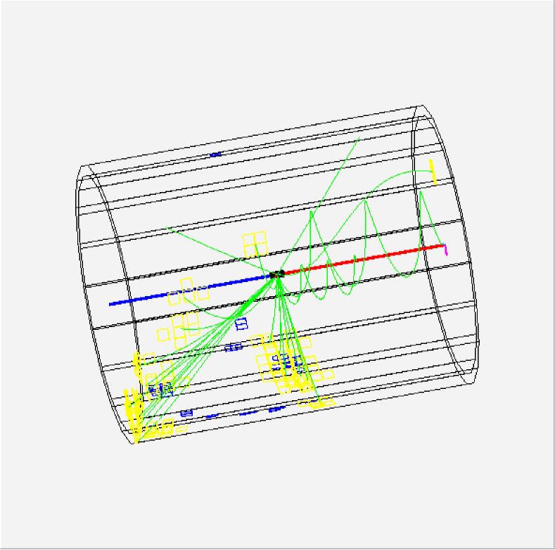
Figure 10: Typical Higgs events; 4 jets, 2 jets + missing, and 2 jets + 2 leptons.

The 4-jet mode is selected by requiring, in principle, a successful forced four-jet clustering and $b$-jet tagging. Selecting two jet-pairs, where the mass of one pair and the missing mass of the other pair are both consistent with $Z$, we could see a clear indication of Higgs even at a low integrated luminosity of 5 fb^-1 (Fig. 11a). In the case of the 2-jet mode, the mass of the Higgs is measured by just calculating the invariant mass of all of the detected particles. Requiring $b$-jet tagging, the missing $p_{t}$ and the missing mass being consistent with $Z\rightarrow\nu\bar{\nu}$, a clean signal can also be seen in this mode (Fig. 11b) at a integrated luminosity of 5 fb^-1. In Fig. 11c, the missing mass of $\mu\bar{\mu}$ disregarding the decay mode of the Higgs is shown. The selection criteria for this mode is just two $\mu$ tracks in good tracking device acceptance, and that their invariant mass is consistent with $m_{z}$. This mode allows a search independently of Higgs decay modes. If the Higgs mass is heavier than about 140 GeV, the Higgs decay to gauge bosons becomes dominant and the search in 4-jet and 2-jet modes must be replaced by searches in gauge boson modes. However, a search in the 2-lepton mode is valid even in this case. Once the design luminosity of the JLC is achieved, the standard Higgs boson will be discovered very easily, as long as it is kinematically accessible.

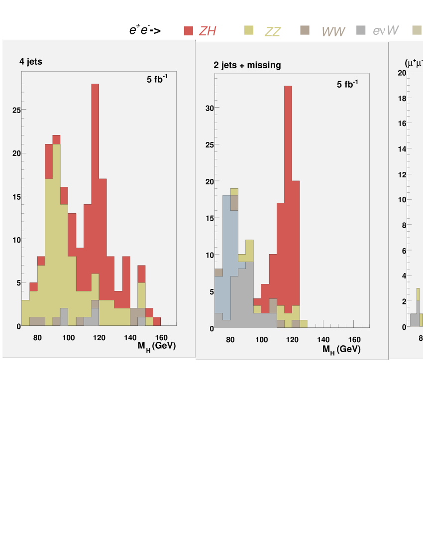
Figure 11: Distribution of Higgs mass for an integrated luminosity of 5 fb^-1 measured in the 4-jet (left), the 2-jet + missing (center), and $\mu\bar{\mu}$ + missing (right) modes. The Higgs process is shown in brown, and the backgrounds are shown by other colors.

If 50 fb^-1 of data is taken, the Higgs signals are evident in all three decay modes, as shown in Fig. 12. Note that 50 fb^-1 of data can be collected for less than one month of the design luminosity of parameter Y.

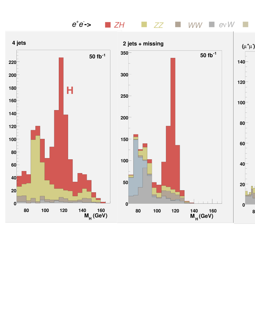
Figure 12: Same as Fig. 11, but for the integrated luminosity of 50 fb^-1.

With two years of operation of the Y parameter, we will be able to accumulate 500 fb^-1 data. With this amount of data, the significance for the standard model Higgs boson is more than 100 if its mass is light (Fig. 13). Even if the standard model Higgs is not the case, a CP-even Higgs boson can be searched irrespective to their decay mode, and if not found, the 5$\sigma$ upper bound of the cross section of 10 fb can be obtained for Higgs mass of up to 200 GeV. This will rule out any GUT model where the Higgs self coupling should not diverge up to GUT energy .

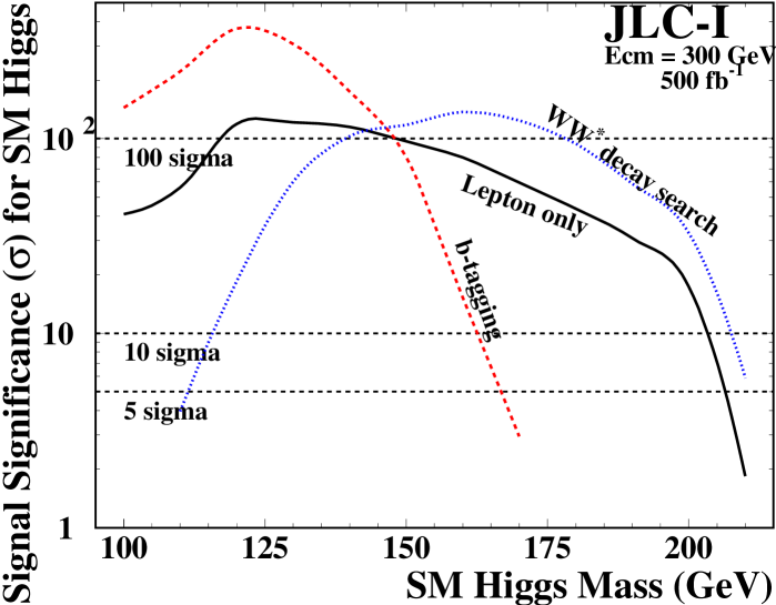
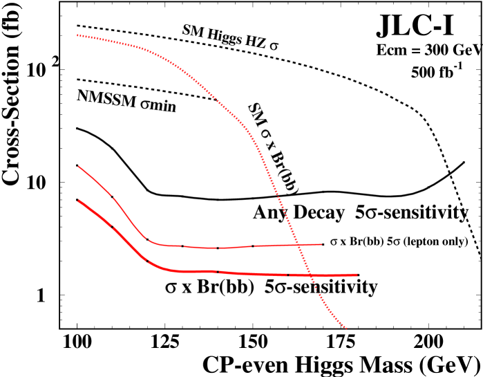
Figure 13: Significances of the standard model Higgs when 500 fb^-1 is accumulated (left) and cross sections of 5$\sigma$ significance for non-standard CP-event Higgs boson (right).

Once a new particle is discovered, the next task is to study its property, such as spin, parity and the strength of $ZZH$ coupling, and to establish the particle as the Higgs. To study the spin, the threshold behavior[6] and the angular distribution of the production and decay are useful.

To measure the mass of Higgs, three methods can be considered: (1) direct mass reconstruction using $H\rightarrow 2jets$ mode, (2) a measurement of the recoil mass using the $Z\rightarrow e\bar{e}/\mu\bar{\mu}$ decay mode, and (3) combined fitting with beam-energy constraints. The natural width of the Higgs is very small (about several MeV unless gauge boson channels dominate) and JLC has a wide energy spread. The detector must have a high resolution at least comparable with the beam energy spread, and be well calibrated using $Z$ signals for example.

A typical mass resolution obtained using the 2-jet mode is shown in Fig. 15. This plot is obtained from an example program of the JSF package[7]. According to a Gauss fit, we obtained a $\sigma$ of 2.7 GeV, while the peak position is shifted about 2.3 GeV. About 15k events are expected for 500 fb^-1. Therefore, a statistical accuracy of less than 30 MeV for the Higgs mass is expected, while the detector must be well calibrated for an unbiased measurement.

Figure 14: Mass distribution of the Higgs boson detected in 2-jet mode. The invariant mass of all particles of selected events are plotted.

Figure 15: Recoil mass distribution of a $\mu^{+}\mu^{-}$ pair of processes $e^{+}e^{-}\rightarrow ZZ$ and $e^{+}e^{-}\rightarrow ZH$, at $\sqrt{s}=250$ GeV. See the texts for more details.

If we use the lepton channel, the mass measurement will be less biased because the Higgs is detected independently of its decay mode as the recoil mass of the lepton pair. However, to achieve high precision measurements of the Higgs mass, a precise tracking device and a narrow initial energy spread is essential. An example, in the case of the distribution of the recoil mass of $\mu$ pair is shown in Fig. 15. In this figure, the signal channel ($e^{+}e^{-}\rightarrow ZH$ for $m_{H}=120$ GeV) is shown together with the background channel ($e^{+}e^{-}\rightarrow ZZ$). Backgrounds below the signal peak are $ZZ$ events at lower collision energies whose energy losses are due to not only the initial state radiation but also the beamstrahlung. The backgrounds can be reduced siginificantly if we apply $b$-tagging to the jets from the Higgs decay, but it is not applied here for the measurement irrespective to the Higgs decay mode. The width of the signal is mainly due to the initial beam energy spread, but is reduces by about 10% if measured at a 10 GeV lower center-of-mass energy due to a kinematical effect[8]. In any case, a mass resolution of about 150 MeV and a precision of the cross section of about 8% are expected from this channel. If we combine the $e^{+}e^{-}$ channel and the integrated luminosity of 500 fb^-1 is considered, a mass resolution of about 45 MeV and a resolution of the cross section of about 2.7% are expected.

The branching ratio of the Higgs boson also needs to be measured, because they may provide hints for physics beyond the standard model. In the standard model, the strength of Higgs fermion coupling is proportional to the fermion mass. However, many models beyond the standard model assumes more than one Higgs doublets; thus the proportionality of the mass and the coupling strength obeys different formula.

When the Higgs decays to a fermion pair, the vertex detector is very powerful to identify its flavor. Several methods, such as $n-sig$ and topological vertex hunting algorithms have been studied and found to be useful to identify Higgs to $c\bar{c}$ decay mode[9] at a precision of 25 %.

The Higgs decay to $WW^{*}$ was studied in the process $e^{+}e^{-}\rightarrow ZH$, where $Z$ decays to $q\bar{q}$ or $\ell^{+}\ell^{-}$ and $H$ decays to $WW^{*}\rightarrow\ell\nu q\bar{q}$. For this study, good jet mass measurements are crucial and lepton channels are useful to reduce combinatorial backgrounds. With the help of a kinematical constraint fit, 5.1% accuracy of $\Delta(\sigma\cdot Br(H\rightarrow WW))/\sigma\cdot Br(H\rightarrow WW^{*})$ is expected for an integrated luminosity of 500 fb^-1.

In the standard model, the total width of the Higgs boson is 2 to 10 MeV for a light Higgs boson of mass from 100 to 140 GeV, thus a directly measurement of the width is difficult. However, by combining the measurement of $\sigma Br(H\rightarrow WW)$ with the measurement of the total cross section $(\sigma_{total})$, the total width $(\Gamma_{total})$ of the Higgs boson can be estimated. This is because $\Gamma_{total}=\Gamma(H\rightarrow WW)Br(H\rightarrow WW)$ and $\Gamma(H\rightarrow WW)$ can be obtained from $\sigma_{total}$ assuming $\Gamma_{HZZ}/\Gamma_{HWW}=(M^{W}\cos\theta_{W}/M_{Z})^{2}$, which is satisfied as long as $W$ and $Z$ are SU(2) gauge bosons. The accuracy of the measurement of the total width can be expressed as

$$\left({\Delta\Gamma_{H}\over\Gamma_{H}}\right)^{2}=\left({\Delta\sigma\cdot BR(H\rightarrow WW)}\over\sigma\cdot BR(H\rightarrow WW)\right)^{2}+\left(2{\Delta\sigma_{total}\over\sigma_{total}}\right)^{2},$$

which becomes about 6.4% for an integrated luminosity of 500 fb^-1. Since heavy particles make a non-negligible contribution to the total width, this measurement provides a tool to prove the particle spectrum at higher energies.

4.2 Top

According to the PDG[12], the mass of the top quark is $174.3\pm 3.2\pm 4.0$ GeV. This implies that the JLC at $\sqrt{s}\sim$ 350 GeV would be a top factory. In addition, because $m_{t}$ is larger than $m_{W}+m_{b}$, the top quark decays to $Wb$ almost 100% of the time in the standard model. The total width ($\Gamma_{t}$) is about 1.4 GeV, which implies that the top decays before entering the non-perturbative QCD region. $\Gamma_{t}$ acts as an infrared cutoff, and clean tests of QCD are possible. Vertecies including top, such as $t\bar{t}\gamma$, $t\bar{t}Z$, $tbW$, $t\bar{t}g$, and $t\bar{t}H$, could be studied, where effects due to new physics beyond the standard model may be found.

At $t\bar{t}$ threshold, $t\bar{t}$ resonances are formed. The lowest resonance ($E_{1S}$) is about 3 GeV below twice the mass of the top quark. There are many resonances below the open threshold, while their mass differences are small, less than, say, 2-times the total width of the top quark. Therefore, although they overlap, a “bump” in the cross section will be seen. From its position in $\sqrt{s}$, we will know the mass of the top quark. From its height and width, information such as the total width of the top quark, and $\alpha_{s}$ can be obtained. On the other hand, the initial state radiation and the beamstrahlung reduce the luminosity usable for resonance production, and the initial beam energy spread smears the peak and/or affects the shape of the peak if the relative spread is larger than about 0.4%.

When a top quark is produced, it decays to $bW$. $W$ decays to a quark pair or a lepton and a neutrino. According to the decay mode of $W$, the signature of $t\bar{t}$ events are categorized as follows:

		Branching ratio
a)	2 $b$ jets + 4 jets from $W$	$\sim 45$%,
b)	2 $b$ jets + 2 jets from $W$ and $\ell\nu$	$\sim 44$%,
c)	2 $b$ jets + 2 pairs of $\ell\nu$	$\sim 11$%.

All modes can be used for measuring the total cross section. The direction and charge of the top quark can be identified in decay modes a) and b), which are used to measure the top quark momentum and the forward-backward asymmetry. The basic cuts to select $t\bar{t}$ events are: (1) event shape cuts such as those on the number of charged particles, the number of jets and thrust, (2) mass cuts to select $W$’s and b jets, (3) requirements of leptons in the cases of b) and c), and (4) $b$ tagging.

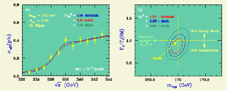
Figure 16: Energy dependence of the $t\bar{t}$ cross section(a) and the expected precision in the plane of the top mass and the total width(b). The 11 point measurements around the threshold, with an integrated luminosity of 1 fb^-1 each are assumed.

A typical measurement of the energy dependence of the $t\bar{t}$ cross section around the threshold region is shown in Fig. 16-(a). In the figure, 11 points of 1 fb^-1 measurement are shown. The lines in the figure are theoretical curves for three cases for the value of $|V_{tb}|$. If $|V_{tb}|$ becomes smaller, $\Gamma_{t}$ becomes smaller and the threshold becomes steeper. The position of the shoulder is determined by the mass of the top. Thus, this measurements could impose a constraint on the plane of the total width and the mass of the top quark, as shown in Fig. 16.

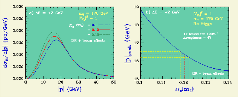
Figure 17: Momentum distribution of the top quark for various values of $\alpha_{S}$ (a) and the peak momentum as a function of $\alpha_{s}$ (b).

When the toponium resonance is formed, the top quark decays to $bW$ before $t\bar{t}$ annihilation. Therefore, if the $t\rightarrow bW$ decay is measured precisely, the top quark momentum in the resonance can be reconstructed to study the toponium potential. This is in contrast to the charmonium and the bottomnium resonance where the $q\bar{q}$ annihilation modes dominate. In Fig. 17, the momentum distribution of the top quark in the toponium resonance is shown for three values of $\alpha_{s}$. The larger is $\alpha_{s}$, the deeper is the toponium potential and the larger is the peak momentum. According to a simulation study, 1$\sigma$ bound for the precision of the peak momentum $(|p|_{peak})$ measurement is about 200 MeV for an integrated luminosity of 100 fb^-1. This value translates to sensitivities of $\Delta\Gamma_{t}/\Gamma_{t}=0.03$ and $\Delta\alpha_{s}(M_{Z})/\alpha_{s}=0.002$, when only one parameter is varied while the others is fixed and the mass of the lowest toponium resonance is known.

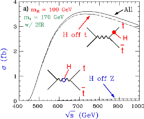
Figure 18: Total cross section of the process $e^{+}e^{-}\rightarrow t\bar{t}H$.

At energies higher than the threshold of the process $e^{+}e^{-}\rightarrow t\bar{t}H$, we can measure the top Yukawa coupling directly. There are two kinds of diagrams contributing to this process at the tree level. The first one includes a diagram where a Higgs boson is radiated off the final-state top or anti-top quarks $(H-off-t)$, and is thus proportional to the top Yukawa coupling. In the second diagram, the Higgs boson is emitted from the $s$-channel Z boson $(H-off-Z)$ and is independent of the top Yukawa coupling. However, the contribution of the $H-off-Z$ diagram is tiny, as shown in Fig. 18.

Considering the light Higgs, where it decays mainly to $b\bar{b}$, the signature of this process is 2 $W$’s and 4 $b$’s, where $W$ decays to $q\bar{q}^{\prime}$ or $\ell\nu$. In a simulation study, 8 jets or 6 jets + $\ell\nu$ final states were selected using jet clustering to find $W$ and $H$ jet pairs. The background processes are $e^{+}e^{-}\rightarrow t\bar{t}$ and $e^{+}e^{-}\rightarrow t\bar{t}Z$ . The former process can be removed by requiring more than two $b$-jets. The latter process is irreducible, and the background is severe if the Higgs mass is close to the mass of $Z$. If $m_{H}=100$ GeV and $m_{t}$=170 GeV, the expected number of events at $\sqrt{s}=700$ GeV is 114, combining 8-jet and 6-jet + $\ell\nu$ mode, while that of the background process is 133, when the integrated luminosity is 100 fb^-1. This translates to an accuracy of the top Yukawa couping of 14%.

4.3 SUSY

Since the radiative correction to the scalar particle is quadratically divergent, the light Higgs boson in GUT models raises the fine-tuning problem[10]. One motivation of SUSY is to solve this problem by introducing super-symmetric particles with mass on the order of 1 TeV or less, and cancel the divergence. Another solution to the fine-tuning problem is to introduce extra dimensions[11].

Obviously, SUSY is broken and the mass spectrum of SUSY particles varies depending on the SUSY breaking models and model parameters[2]. Since SUSY particle searches at JLC is model independent, their measurements are useful to distinguish various models.

In gravity mediated models, gaugino masses are unified at the GUT scale, but at the EW scale, charginos and neutralinos are lighter than the gluino ($m_{\tilde{\chi}}\sim\frac{1}{3}m_{\tilde{g}}$) because they receive radiative corrections differently. Accordingly, the lightest neutralino ($\tilde{\chi}_{1}^{0}$) is expected to be the lightest SUSY particle. Similarly, the right-handed fermion is expected to be the lightest matter fermion ($m_{\tilde{f}_{R}}<m_{\tilde{f}_{R}}<m_{\tilde{q}}$). Therefore, channels to search for sparticles are the right-handed sfermion($\tilde{f}_{R}$) decays to the right-handed fermion($f_{R}$) and LSP($\tilde{\chi}^{0}_{1}$) or the chargino decays ($\tilde{\chi}^{\pm}$) to the gauge bosons($W^{\pm}$) and LSP($\tilde{\chi}^{0}_{1}$). The event signature of the sparticle production is a missing $p_{t}$.

In anomaly mediated models, SUSY symmetry is broken by loop effects. The mass differences among gauginos and fermions are usually small, though the neutralino is expected to be LSP. If the mass difference of LSP and the next LSP is large, the signature of the sparticle production is a missing $p_{t}$. It is similar to the case of the gravity mediated models. However, if the mass difference is small, particle multiplicities of events are small and special care must be taken to find sparticles.

On the contrary, in the gauge mediated models, the gravitino is the LSP and the next lightest sparticles, NLSP, can be $\tilde{\chi}_{1}^{0}$, lightest stau ($\tilde{\tau_{1}}$), or right-handed electron ($\tilde{e}_{R}$) depending on model parameters. Their lifetimes also depend on the parameters. If the lifetime of the NLSP is short and decays near to the interaction point, the event signature is the missing $p_{t}$ due to energies taken away by the gravitino. If it is long, but decayed, with in the detector, spectacular events, such as off-vertex $\gamma$ or $\tau$ tracks may be seen. If their lifetime is very long and does not decay within the detector, the NLSP momentum is not detected. In this case, we needs to search for the next-to-next LSP to NLSP decays, and the event signature is again the missing $p_{t}$.

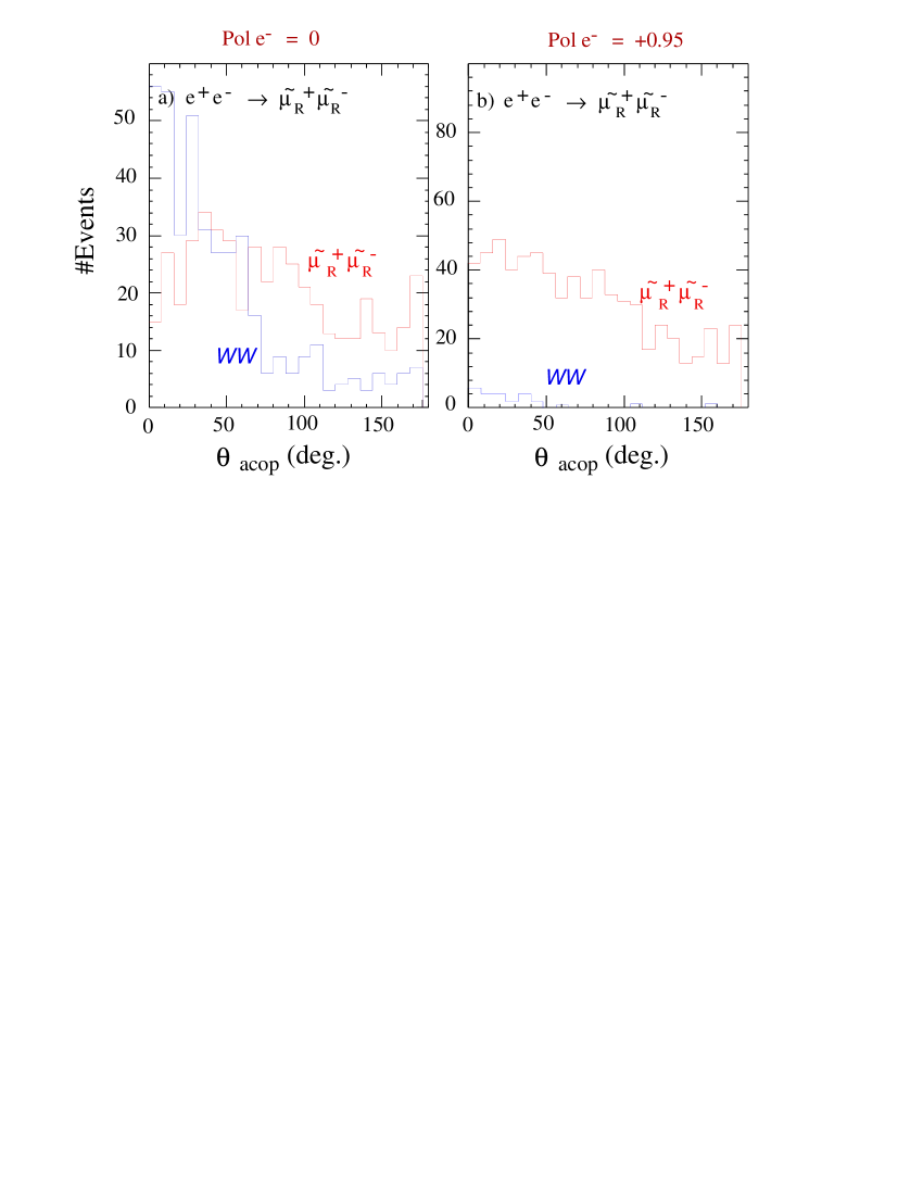
Figure 19: Examples of the acoplanarity distribution of smuon pair production for without a polarized beam (a) and with a polarized $e^{-}$ beam. The Monte Calro data corresponds to an integrated luminosity of 20 fb^-1 at $\sqrt{s}=350$ GeV.

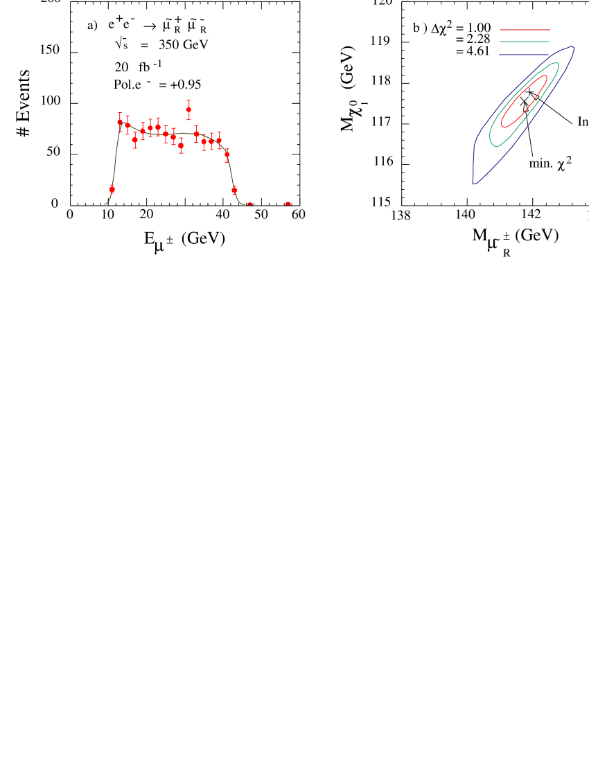
Figure 20: (a) Energy distribution of muons from smuon decays and (b) contours in the $m_{\tilde{\mu}}-m_{\tilde{chi}^{0}_{1}}$ plane obtained from a fit to the energy distribution.

In any case, the detection of SUSY particle is easy at JLC once the kinematical threshold is exceeded, and no model assumption, such as mass spectrum etc, is required for its detection. Once they are discovered, the masses and couplings will be precisely measured from which we will study the SUSY breaking mechanism and underlying physics.

As an example of SUSY studies at JLC, searches and studies of right handed scalar leptons are discussed below. We consider the process, $e^{+}e^{-}\rightarrow\tilde{\mu}^{+}\tilde{\mu}^{-}$, where $\tilde{\mu}^{\pm}$ decays to $\mu^{\pm}$ and $\tilde{\chi}^{0}_{1}$. The signature of this event is a missing $p_{t}$ due to an un-detected momentum of $\tilde{\chi}^{0}_{1}$, which leads to acoplanar $\mu^{\pm}$ events. The distribution of the acoplanarity angle($\Theta_{acop}$) is shown in Fig. 19. Since only the $B$ boson (the gauge boson of $U(1)_{Y}$ group) contributes to smuon($\tilde{\mu}^{\pm}$) production, the use of a right-handed electron beam enhances the signal twice, while it reduces the major $W^{+}W^{-}$ backgrounds completely, as can be seen in the Figure.

In the decay of smuon, the energy distribution of muon is flat as smuon is a scalar particle. The end points of its energy distribution are kinematically fixed by the masses of the parent and daughter particles. Namely, the masses of smuon and the LSP can be determined from the end points of the smuon energy distribution. An example of the energy distribution is shown in Fig. 20. For the case used for a Monte Calro study, the expected mass resolution of smuon is $\pm 0.8$ GeV, and that for LSP is $\pm 0.6$ GeV if the 20 fb^-1 data is corrected at $\sqrt{s}=350$ GeV.

If the universal scalar mass is the case such as expected in models like gravity mediated models, not only the smuon but also the selectron is produced at a similar energy. In this case, the signature is acoplanar $e^{\pm}$, and can be easily distinguished from an acoplanar $\mu^{\pm}$ signal. The mass of selectron is measured from the end points of $e^{\pm}$ energy distribution. Combining the mass measurement of smuon, the model assumption of the universal scalar mass can be easily tested.

       

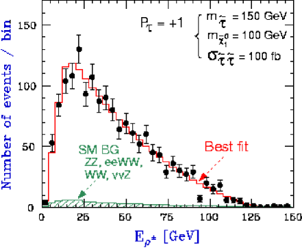
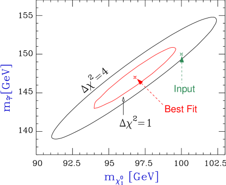
Figure 21: a) Energy distribution of the final state hadrons selected as $\rho$’s from stau decays shown together with the best fit, when $10^{4}$ $\tilde{\tau}_{1}$ pairs are produced and decay in the $\tilde{chi}^{0}_{1}\tau_{R}$ mode, and b) $\Delta\chi^{2}=1,4$ contour in the $m_{\tilde{\chi}^{0}_{1}}-m_{\tilde{\tau}_{1}}$ mode.

Concerning the third generation slepton, stau($\tilde{\tau}$), its mass matrix contains large off-diagonal elements since the tau mass ($m_{\tau}$) is much heavier than the other leptons. This produces a large mixing between left-handed and right-handed stau and a large mass splitting between the mass eigen states of the stau ($\tilde{\tau}_{1}$, $\tilde{\tau}_{2}$) is expected. Thus, $\tilde{\tau}_{1}$ may be the lightest charged SUSY particle.

The signature of stau pair production is a pair of leptons or low multiplicity hadron jets from tau decays. Since a neutrino is produced in tau decay, the energy distribution of the observed leptons or hadron jets is not uniform, as with the case of the smuon or selectron. Still, the energy distribution of the decayed daughter reflects the masses of the stau and neutralino and we will be able to determine their masses. An example of an energy distribution of $\rho$ mesons from tau decay is shown in Fig. 21-(a). From the fit, the mass of the stau can be determined at 2% precission using a sample corresponding to an integrated luminosity of 100 fb^-1.

Generally, the total cross section of the right handed slepton and the left handed slepton is different due to the difference of the weak hyper charge. If $\sqrt{s}>\!\!>m_{Z}$ and the beam electron is right-handed, only a $B$ boson of the $U(1)_{Y}$ gauge group contributes to slepton production. In this case, the total cross section of the right handed slepton is four times larger than that of the left handed slepton. Thus if the mass is fixed, the cross section of the lightest stau($\tilde{\tau}_{1}$) is determined by the mixing ratio of $\tilde{\tau}_{R}$ and $\tilde{\tau}_{L}$ ($\sin\theta_{\tilde{\tau}}$). To put it another way, the mixing angle of the stau sector can be measured using a measurement of the total cross section of a stau. According to a monte calro simulation of 100 fb^-1 luminosity at 500 GeV, a 6.5% precission measurement of $\sin\theta_{\tilde{\tau}}$ is expected.

There is also a mixing in the stau decay, which decays to a tau and a neutralino. The neutralino consists of a Bino($\tilde{B}^{0}$), a Wino($\tilde{W}_{3}^{0}$) and Higgsinos($\tilde{H}_{1}^{0}$ , $\tilde{H}_{2}^{0}$). If a stau interacts with a Bino or a Wino, a tau with the opposite helicity is produced. If a stau interacts with a Higgsino, a tau with the same helicity is produced. As a result, the polarization of the daughter tau is determined by the mixing angles of the neutralino and the stau mixing angle. This property can be exploited to determine $\tan\beta$[13].

5 Summary

In this talk, after a short summary of the JLC accelerator and the detector, selected topics on physics of the Higgs, Top and SUSY particles are presented. The initial goal of JLC is to achieve a center-of-mass energy of 500 GeV with a luminosity of about $2.5\times 10^{34}/cm^{2}/s$. JLC will be a Top factory. If the Higgs boson is as light as expected from recent electroweak data, JLC will also be a Higgs factory. Some SUSY particles may be observed at JLC. A clean experimental environment will allow us to provide definite results on studies of these particles. It will be an indispensable basis for our understanding of the physics beyond the standard model. The beginning of the JLC experiment is highly awaited.

Acknowledgments
This talk is based on the ACFA report[2]. The author would like to thank the members of ACFA Joint Linear Collider Physics and Detector working group.

References

- [1] For ACFA activities, see http://acfahep.kek.jp/ and links therein.
- [2] K. Abe, et al., Particle Physics Experiments at JLC, KEK Report 2001-11, August 2001.
- [3] K. Yokoya, private communication.
- [4] ALEPH, DELPHI, L3 and OPAL Collaborations, CERN-EP/2001-055, July 2001 (hep-ex/0107029).
- [5] The LEP Electroweak Working Group and the SLD Heavy Flavour Group, CERN-EP 2001-098, December 2001 (hep-ex/0112021).
- [6] D.J. Miller, S.Y. Choi, B. Eberle, M.M. Mühlleitner, and P.M. Zerwas, Phys. Lett. B505(2001)149.
- [7] A. Miyamoto, p.646, in Proceedings of LCWS 2000, Batavia, USA, 2000, edited by Adam Para and H.Eugene Fisk (AIP Conference Proceedings Vol. 578 ); http://www-jlc.kek.jp/subg/offl/jsf.
- [8] A. Miyamoto, p.833, in Proceedings of LCWS 2000, Batavia, USA, 2000, edited by Adam Para and H.Eugene Fisk (AIP Conference Proceedings Vol. 578 ).
- [9] G.B. Yu, J.S Kan, A. Miyamoto, H.B. Park, in these proceedings.
- [10] See for example, C.H.L. Smith, Phys. Rep. 105(1984)53 and references therein.
- [11] G. Landsberg, p.1150, in Proceedgins of the 30th International Conference on High Energy Physics, Osaka, Japan, 2000, edited by C.S. Lim and T. Yamanaka (World Scientific), and references therein.
- [12] Particle Data Group, D.E. Groom, et al., Euro. Phys. J. 15(2000)26.
- [13] M. Nojiri, K. Fujii, T. Tsukamoto, Phys. Rev. 54(1996)6756.