AN IMPROVED STUDY OF THE STRUCTURE OF
e⁺e^- $\rightarrow$$b\overline{b}g$ EVENTS AND LIMITS ON THE ANOMALOUS
CHROMOMAGNETIC COUPLING OF THE $b$-QUARK^∗

ABSTRACT

The structure of three-jet e⁺e^-$\rightarrow$$b\overline{b}g$ events has been studied using hadronic $Z^{0}$ decays recorded in the SLD experiment at SLAC. Three-jet final states were selected and the CCD-based vertex detector was used to identify two of the jets as $b$ or $\overline{b}$; the remaining jet in each event was tagged as the gluon jet. Distributions of the gluon energy and polar angle with respect to the electron beam were measured over the full kinematic range, and used to test the predictions of perturbative QCD. We find that beyond-leading-order QCD calculations are needed to reproduce the features seen in the data. The energy distribution is sensitive to an anomalous $b$ chromomagnetic moment $\kappa$ at the $b\bar{b}g$ vertex. We measured $\kappa$ to be consistent with zero and set 95% C.L. limits on its value, $-0.06<\kappa<0.04$.

Submitted to Physical Review D

^∗ Work supported in part by Department of Energy contract DE-AC03-76SF00515.

1 Introduction

The observation of $e^{+}e^{-}$ annihilation into final states containing three hadronic jets, and their interpretation in terms of the process $e^{+}e^{-}\rightarrow q\overline{q}g$ [1], provided the first direct evidence for the existence of the gluon, the gauge boson of the theory of strong interactions, Quantum Chromodynamics (QCD). In subsequent studies the jets were usually energy ordered, and the lowest-energy jet was assigned as the gluon; this is correct roughly 80% of the time, but preferentially selects low-energy gluons. If the gluon jet can be tagged explicitly, event-by-event, the full kinematic range of gluon energies can be explored, and more detailed tests of QCD can be performed [2]. Due to advances in vertex-detection this is now possible using e⁺e^-$\rightarrow$$b\overline{b}g$ events. The large mass and relatively long lifetime, $\sim$ 1.5 ps, of the leading $B$ hadron in $b$-quark jets [3] lead to decay signatures that distinguish them from lighter-quark ($u$, $d$, $s$ or $c$) and gluon jets. We used our charge-coupled-device (CCD)-based vertex detector (VXD) [4] to identify in each event the two jets that contain the $B$ hadrons, and hence to tag the gluon jet. This allowed us to measure the gluon energy and polar-angle distributions over the full kinematic range.

Additional motivation to study the $b\overline{b}g$ system has been provided by measurements involving inclusive $Z^{0}$$\rightarrow$$b\bar{b}$ decays. Several early determinations [5] of $R_{b}$ = $\Gamma(Z^{0}\rightarrow$$b\bar{b}$ )/$\Gamma(Z^{0}\rightarrow$$q\overline{q}$ ) differed from Standard Model (SM) expectations at the few standard deviation level. More recently it has been noted that the LEP measurement of the $b$-quark forward-backward asymmetry, $A_{FB}^{b}$, lies roughly 2.5 standard deviations below the SM expectation. Since one expects new high-mass-scale dynamics to couple to the massive third-generation fermions, these measurements have aroused considerable interest and speculation. We have therefore investigated in detail the strong-interaction dynamics of the $b$-quark. We have compared the strong coupling of the gluon to $b$-quarks with that to light- and charm-quarks [6], as well as tested parity (P) and charge$\oplus$parity (CP) conservation at the $b\overline{b}g$ vertex [7]. We have also studied the structure of $b\overline{b}g$ events, via the distributions of the gluon energy and polar angle with respect to (w.r.t.) the beamline [8], using the JADE algorithm [9] for jet definition.

Here we update the $b\overline{b}g$ structure measurements using a data sample more than 3 times larger than in our earlier study, and recorded in the upgraded vertex detector, which allowed us to improve significantly the gluon-jet tagging. In addition we extended our study to include the Durham, Geneva, E, E0 and P algorithms [10] to define jets, and compared these results with perturbative QCD predictions. This constitutes a more detailed test of QCD and enabled us to study systematic effects arising from the jet definition algorithm.

Furthermore, we have used these data to study possible deviations from QCD in the form of radiative corrections induced by new physics, in terms of the $b$-quark chromomagnetic moment. In QCD this is induced at the one-loop level and is of order $\alpha_{s}$/$\pi$. A more general $b\overline{b}g$ Lagrangian term with a modified coupling [11] may be written:

$${\cal L}^{b\overline{b}g}=g_{s}\overline{b}T_{a}\{\gamma_{\mu}+\frac{i\sigma_{\mu\nu}k^{\nu}}{2m_{b}}(\kappa-i\tilde{\kappa}\gamma_{5})\}bG_{a}^{\mu},$$ (1)

where $\kappa$ and $\tilde{\kappa}$ parametrize the anomalous chromomagnetic and chromoelectric moments, respectively, which might arise from physics beyond the SM. The effects of the chromoelectric moment are sub-leading w.r.t. those of the chromomagentic moment, so for convenience we set $\tilde{\kappa}$ to zero. A non-zero $\kappa$ would be observable as a modification [11] of the gluon energy distribution in $b\overline{b}g$ events relative to the standard QCD case. We have used our precise measurements of the gluon energy distributions to set the most stringent limits on $\kappa$.

2 $b\bar{b}g$ Event Selection

We used hadronic decays of $Z^{0}$ bosons produced by $e^{+}e^{-}$ annihilations at the SLAC Linear Collider (SLC) and recorded in the SLC Large Detector (SLD) [12]. The criteria for selecting hadronic $Z^{0}$ decays and the charged tracks used for flavor-tagging are described in [6, 13]. Three-jet events were selected using iterative clustering algorithms applied to the set of charged tracks in each event. We used in turn the JADE, Durham, E, E0, P and Geneva algorithms. The respective scaled-invariant-mass, $y_{cut}$, values were chosen to maximise the statistical power of the measurement, while keeping systematic errors small; they are shown in Table 1.

Jet algorithm	$y_{cut}$ value	# 3-jet events	efficiency
JADE	0.025	57341	12.2%
Durham	0.0095	46432	12.1%
E	0.0275	66848	11.7%
E0	0.0275	54163	11.2%
P	0.02	60387	12.0%
Geneva	0.05	40895	12.8%

Table 1: Number of selected 3-jet events, and gluon-jet tagging efficiency (see text), for each algorithm. The statistical error on the efficiency is roughly 0.04%.

Events classified as 3-jet states were retained if all three jets were well contained within the barrel tracking system, with polar angle $|\cos\theta_{jet}|$ $\leq$ 0.80. In addition, in order to select planar 3-jet events, the sum of the angles between the jet axes was required to be between 358 and 360 degrees. From our 1996-98 data samples, comprising roughly 400,000 hadronic $Z^{0}$ decays, the numbers of selected events are shown in Table 1. In order to improve the energy resolution the jet energies were rescaled kinematically according to the angles between the jet axes, assuming energy and momentum conservation and massless kinematics. The jets were then labelled in order of energy such that $E_{1}>E_{2}>E_{3}$.

Charged tracks with high quality information in the VXD as defined in [6] were used to tag $b\overline{b}g$ events. For each such track we examined the impact-parameter, $d$, w.r.t. the interaction point (IP). The resolution on $d$ is given by $\sigma_{d}=$7.7$\oplus$29$/p\sin^{3/2}\theta$ $\mu$m in the plane transverse to the beamline, and 9.6$\oplus$29$/p\sin^{3/2}\theta$ $\mu$m in any plane containing the beamline, where $p$ is the track momentum in GeV/c, and $\theta$ the polar angle, w.r.t. the beamline.

Jets containing heavy hadrons were tagged using a topological algorithm [14] applied to the set of tracks associated with each jet. A track density function was calculated, and a region of high total track density well separated from the IP was identified as a vertex from the decay of a heavy hadron. For each vertex, the $p_{t}$-corrected invariant mass [14], $M_{p_{t}}$, was calculated using the set of tracks associated with the vertex, assuming the charged pion mass, and the vertex axis, defined to be the vector from the IP to the reconstructed vertex position. Fig. 1 shows the $M_{p_{t}}$ distributions separately for vertices found in jets 1, 2 and 3 using, for illustration, the JADE algorithm; results using the other algorithms (not shown) are qualitatively similar. The simulated contributions from true $b$, $c$, light and gluon jets are indicated; the $c$, light and gluon jets populate predominantly the region $M_{p_{t}}$ $<$ 2 GeV/$c^{2}$. Events were retained in which exactly two jets contained such a vertex, and at least one of them had $M_{p_{t}}$ $>$ 2 GeV/c². In order to suppress events in which a single $B$-hadron decay gave rise to two reconstructed vertices, the cosine of the angle between the two vertex axes was required to be less than 0.7, and the distance between the vertices, projected in a plane perpendicular to the beamline, was required to exceed 0.12 cm. Roughly 1.1% of the event sample was rejected by these cuts. In each selected event the jet without a vertex was tagged as the gluon jet.

For each algorithm, the number of tagged jets is shown in Table 2; also shown, in Table 1, is the efficiency for tagging the gluon jet correctly in true $b\overline{b}g$ events, which was calculated using a simulated event sample generated with JETSET 7.4 [15], with parameter values tuned to hadronic $e^{+}e^{-}$ annihilation data [16], combined with a simulation of $B$-decays tuned to $\Upsilon$(4S) data [17] and a simulation of the detector. For the JADE algorithm, for example, the efficiency peaks at about 15% for 18 GeV gluons. Below 18 GeV the efficiency falls, to as low as 3%, since lower-energy gluon jets are sometimes merged with the parent $b$-jet by the jet-finder. Above 18 GeV the efficiency falls, to as low as 5%, since at higher gluon energies the correspondingly lower-energy $b$-jets are more difficult to tag, and there is also a higher probability of losing a jet outside the detector acceptance. Results for the other algorithms are qualitatively similar. The systematic error associated with the tagging efficiency was small and was explicitly taken into account by the procedure for estimating systematic uncertainties that is described in Section 3.

	JADE		Durham		E
jet label	# jets	purity (%)	# jets	purity (%)	# jets	purity (%)
3	4349	98.0	2952	97.0	5246	97.5
2	740	90.2	890	92.4	1007	85.4
1	150	71.0	138	73.4	148	70.8
	E0		P		Geneva
jet label	# jets	purity (%)	# jets	purity (%)	# jets	purity (%)
3	4027	98.0	4654	98.0	3491	93.9
2	692	90.2	795	90.7	692	86.7
1	151	70.7	155	72.1	181	63.4

Table 2: Tagging purities (see text).

For each algorithm the tagging purities, defined as the fraction of selected 3-jet events in which the two vertices were found in the two jets containing the true $B$ hadrons, are listed by gluon-jet number in Table 2. We formed the distributions of two gluon-jet observables, the scaled energy $x_{g}=2E_{\rm{gluon}}/\sqrt{s}$, and the polar angle w.r.t. the beamline, $\theta_{g}$. For illustration, for the JADE algorithm the distributions are shown in Fig. 2; the simulation is also shown; it reproduces the data. Results for the other algorithms (not shown) are qualitatively similar.

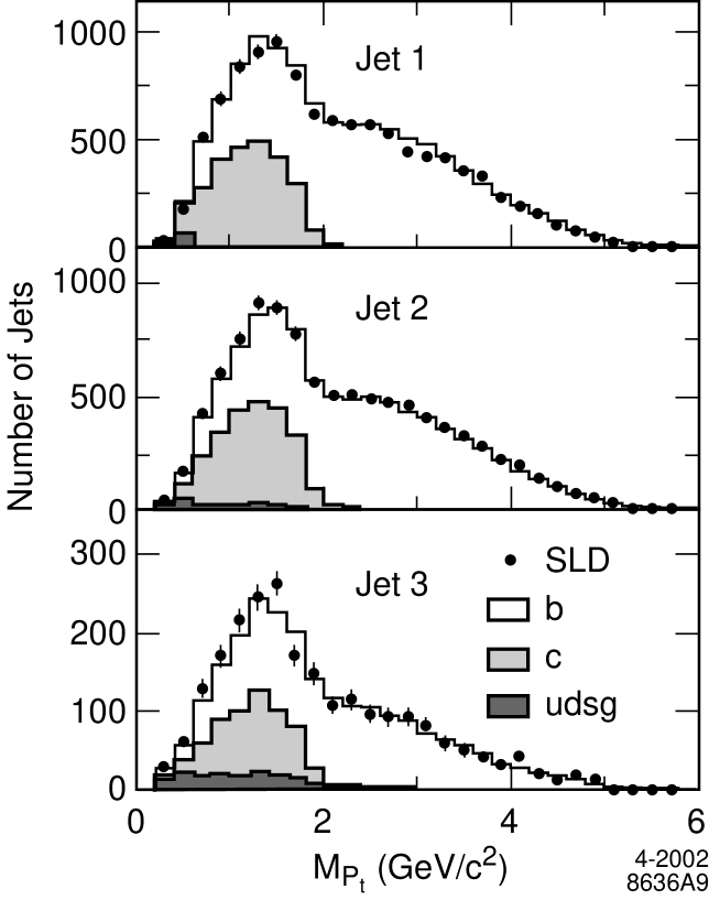
Figure 1: The $M_{pt}$ distributions for vertices found in selected 3-jet events, defined using the JADE algorithm, labelled according to jet energy (dots); errors are statistical. Histograms: simulated distributions for different jet flavors. Events were selected by requiring that at least two jets contain a vertex, at least one of which must satisfy $M_{pt}$ $>$ 2 GeV/$c^{2}$ (see text).

.

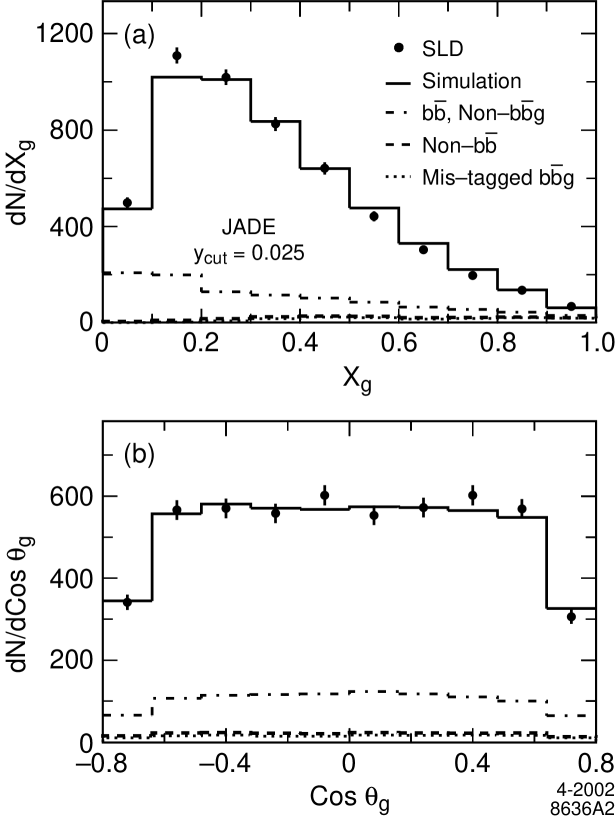
Figure 2: Raw measured distributions of (a) $x_{g}$ and (b) cos$\theta_{g}$ (dots) defined using the JADE algorithm; errors are statistical. Histograms: simulated distributions including background contributions.

The backgrounds were estimated using the simulation and are of three types: non-$b\bar{b}$ events; $b\bar{b}$ but non-$b\overline{b}g$ events; and mis-tagged true $b\overline{b}g$ events. Their contributions are shown in Fig. 2 for the JADE case. Results for the other algorithms (not shown) are qualitatively similar. For each algorithm, the non-$b\bar{b}$ events make up roughly 1$\%$ of the selected sample and are dominated by $c\overline{c}g$ events; roughly 70% of these had the gluon jet correctly tagged, and the remainder comprises events in which the gluon split into a $c\bar{c}$ or $b\bar{b}$ , which yielded a real secondary vertex in the ‘wrong’ jet. Mis-tagged events, in which the gluon jet was mis-tagged as a $b$ or $\bar{b}$-jet and one of the true $b$- or $\bar{b}$-jets enters into the measured gluon distributions, comprise roughly 3% of the sample; roughly two thirds of these events contain a gluon splitting into $c\bar{c}$ or $b\bar{b}$ . These two backgrounds are negligible except in the highest $x_{g}$ bin.

For all algorithms the dominant background (eg.for JADE, roughly 16% of the sample) is formed by $b\bar{b}$ but non-$b\overline{b}g$ events. These are true $b\bar{b}$ events that were not classified as 3-jet events at the parton level, but were reconstructed and tagged as 3-jet $b\overline{b}g$ events in the detector using the same jet algorithm and $y_{cut}$ value. In a parton-level 2-jet event this can arise from the broadening of the particle flow around the original $b$ and $\overline{b}$ directions due to hadronization and weak decay; in particular, the relatively high-transverse-momentum $B$-decay products can cause the jet-finder to reconstruct a ‘fake’ third jet, which is almost always assigned as a (low-energy) gluon jet. In addition, an event classified as 4-jet at the parton level may, due to the overlap of their hadronization products, have two of its jets combined in the detector by the jet-finder. In this case the combined jet is usually tagged as a gluon jet . Since the calculations with which we compare below are not reliable for 4-jet events, we consider such events to be a background.

3 Correction of the Data

For each algorithm, the distributions were corrected to obtain the true gluon distributions $D^{true}(X)$ by applying a bin-by-bin procedure: $D^{true}(X)=C(X)\;(D^{raw}(X)-B(X))$, where $X$ = $x_{g}$ or cos$\theta_{g}$, $D^{raw}(X)$ is the raw distribution, $B(X)$ is the background contribution, and $C(X)\equiv D^{true}_{MC}(X)/D^{recon}_{MC}(X)$ is a correction that accounts for the efficiency for accepting true $b\overline{b}g$ events into the tagged sample, as well as for bin-to-bin migrations caused by hadronization, the resolution of the detector, and bias of the jet-tagging technique. Here $D^{true}_{MC}(X)$ is the true distribution for MC-generated $b\overline{b}g$ events, and $D^{recon}_{MC}(X)$ is the resulting distribution after full simulation of the detector and application of the same analysis procedure as applied to the data.

The fully-corrected distributions are shown in Figs. 3, 4, 5, 6, 7, and 8. Since, in an earlier study [6], we verified that the overall rate of $b\overline{b}g$ -event production is consistent with QCD expectations, we normalised the gluon distributions to unit area and we study further the distribution shapes. In each case the peak in $x_{g}$ is a kinematic artefact of the jet-finding algorithm, which ensures that gluon jets are reconstructed with a non-zero energy, and it depends on the $y_{cut}$ value. The cos$\theta_{g}$ distributions are very nearly flat, in contrast to the $1+\cos^{2}\theta$ behavior for quark jets.

.

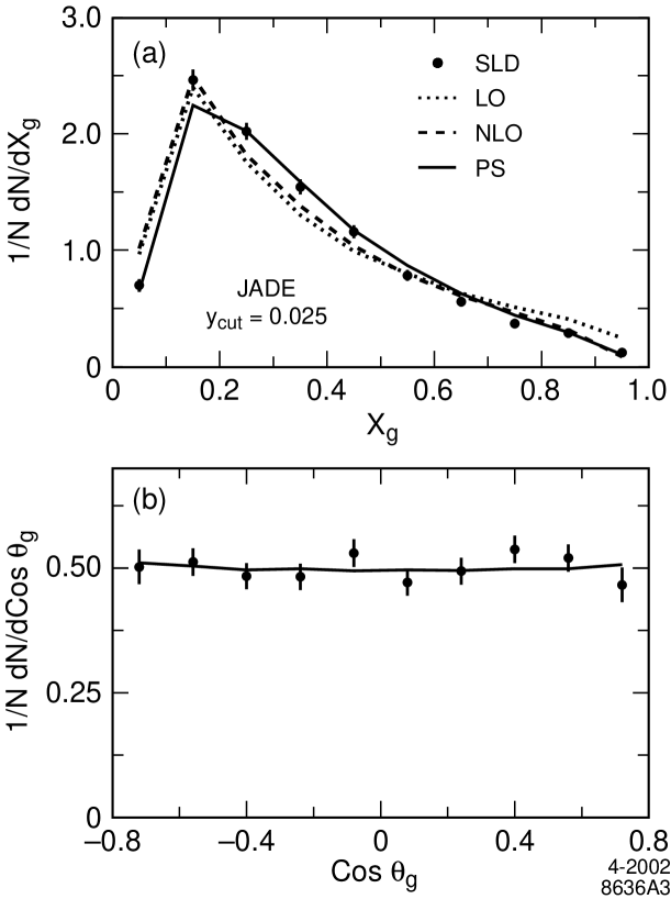
Figure 3: Corrected distributions of (a) $x_{g}$ and (b) cos$\theta_{g}$ (dots) defined using the JADE algorithm; the error bars represent the sum in quadrature of the statistical and systematic errors. Perturbative QCD predictions (see text) are shown as lines joining entries plotted at the respective bin centers.

.

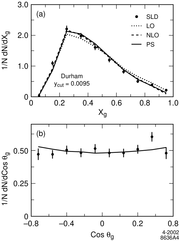
Figure 4: Corrected distributions of (a) $x_{g}$ and (b) cos$\theta_{g}$ (dots); defined using the Durham algorithm; the error bars represent the sum in quadrature of the statistical and systematic errors. Perturbative QCD predictions (see text) are shown as lines joining entries plotted at the respective bin centers.

.

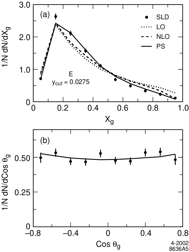
Figure 5: Corrected distributions of (a) $x_{g}$ and (b) cos$\theta_{g}$ (dots); defined using the E algorithm; the error bars represent the sum in quadrature of the statistical and systematic errors. Perturbative QCD predictions (see text) are shown as lines joining entries plotted at the respective bin centers.

.

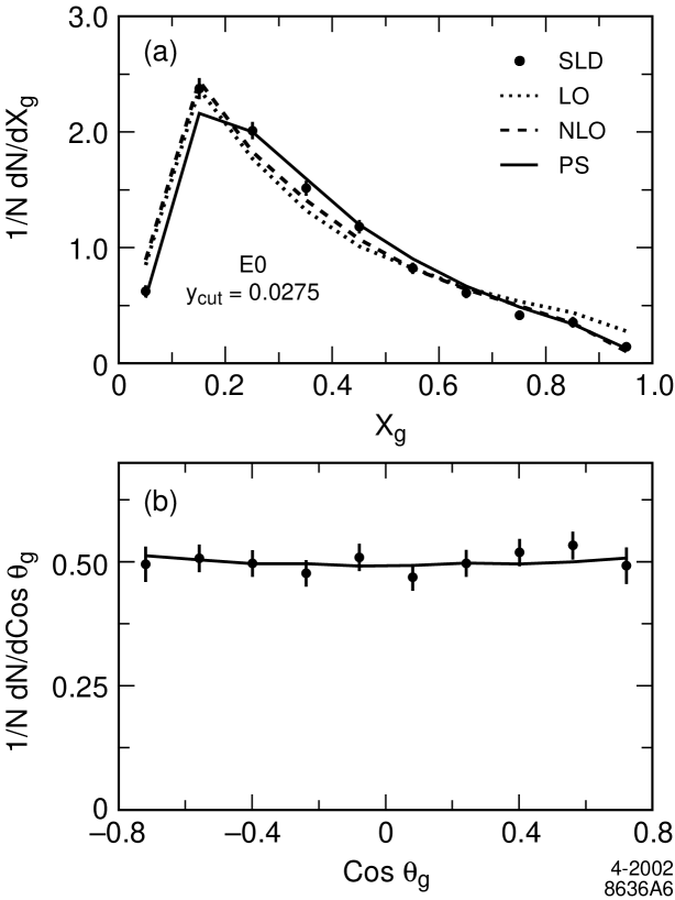
Figure 6: Corrected distributions of (a) $x_{g}$ and (b) cos$\theta_{g}$ (dots); defined using the E0 algorithm; the error bars represent the sum in quadrature of the statistical and systematic errors. erturbative QCD predictions (see text) are shown as lines joining entries plotted at the respective bin centers.

.

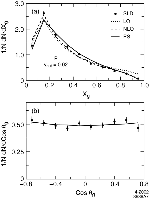
Figure 7: Corrected distributions of (a) $x_{g}$ and (b) cos$\theta_{g}$ (dots); defined using the P algorithm; the error bars represent the sum in quadrature of the statistical and systematic errors. Perturbative QCD predictions (see text) are shown as lines joining entries plotted at the respective bin centers.

.

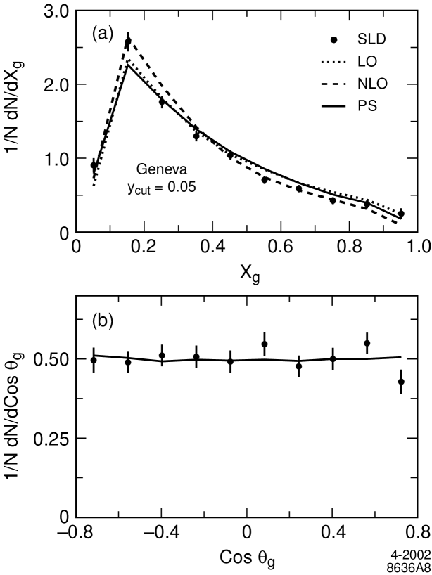
Figure 8: Corrected distributions of (a) $x_{g}$ and (b) cos$\theta_{g}$ (dots); defined using the Geneva algorithm; the error bars represent the sum in quadrature of the statistical and systematic errors. Perturbative QCD predictions (see text) are shown as lines joining entries plotted at the respective bin centers.

We have considered sources of systematic uncertainty that potentially affect our results. These may be divided into uncertainties in modelling the detector and uncertainties in the underlying physics modelling. To estimate the first case we systematically varied the track and event selection requirements, as well as the track-finding efficiency [6, 13], the momentum and dip angle resolution, and the probability of finding a fake vertex in a jet. In the second case parameters used in our simulation, relating mainly to the production and decay of charm and bottom hadrons, were varied within their measurement errors [18]. For each variation the data were recorrected to derive new $x_{g}$ and cos$\theta_{g}$ distributions, and the deviation w.r.t. the standard case was assigned as a systematic uncertainty. Although many of these variations affect the overall tagging efficiency, most had little effect on the energy or polar angle dependence, and no variation affects the conclusions below. The largest contributions to the error arose from the measurement uncertainties on the probability for gluon splitting into $b\bar{b}$  (which dominates around $x_{g}$ $\sim$ 0.5) or $c\bar{c}$  (which dominates for $x_{g}$ $>$ 0.7).

All uncertainties were conservatively assumed to be uncorrelated and were added in quadrature in each bin of $x_{g}$ and cos$\theta_{g}$. In any bin the systematic error is typically much smaller than the statistical error. The data points with their total error bars are shown in Figures 3, 4, 5, 6, 7, 8; the data are listed in Tables 3 and 4. In addition, as cross-checks, for each algorithm the $y_{cut}$ value and the $M_{p_{t}}$ cut were varied around their respective default values; in no case did our conclusions change.

1/N dN/d$x_{g}$
$x_{g}$ range		JADE			Durham			E
0.0–	0.1	0.697$\pm$	0.055 $\pm$	0.001	0.000$\pm$	0.000 $\pm$	0.000	0.712$\pm$	0.045 $\pm$	0.001
0.1–	0.2	2.461$\pm$	0.093 $\pm$	0.002	1.093$\pm$	0.073 $\pm$	0.005	2.634$\pm$	0.091 $\pm$	0.005
0.2–	0.3	2.021$\pm$	0.074 $\pm$	0.003	2.209$\pm$	0.106 $\pm$	0.011	2.111$\pm$	0.075 $\pm$	0.010
0.3–	0.4	1.544$\pm$	0.064 $\pm$	0.006	1.982$\pm$	0.093 $\pm$	0.018	1.574$\pm$	0.065 $\pm$	0.015
0.4–	0.5	1.158$\pm$	0.056 $\pm$	0.007	1.606$\pm$	0.083 $\pm$	0.021	1.111$\pm$	0.055 $\pm$	0.019
0.5–	0.6	0.783$\pm$	0.047 $\pm$	0.008	1.196$\pm$	0.072 $\pm$	0.015	0.684$\pm$	0.045 $\pm$	0.024
0.6–	0.7	0.559$\pm$	0.042 $\pm$	0.008	0.814$\pm$	0.060 $\pm$	0.012	0.493$\pm$	0.041 $\pm$	0.029
0.7–	0.8	0.371$\pm$	0.038 $\pm$	0.009	0.501$\pm$	0.049 $\pm$	0.010	0.337$\pm$	0.039 $\pm$	0.033
0.8–	0.9	0.287$\pm$	0.038 $\pm$	0.012	0.385$\pm$	0.048 $\pm$	0.011	0.231$\pm$	0.038 $\pm$	0.032
0.9–	1.0	0.119$\pm$	0.028 $\pm$	0.013	0.214$\pm$	0.043 $\pm$	0.013	0.114$\pm$	0.026 $\pm$	0.020
$x_{g}$ range		E0			P			Geneva
0.0–	0.1	0.620$\pm$	0.050 $\pm$	0.001	1.362$\pm$	0.092 $\pm$	0.001	0.912$\pm$	0.096 $\pm$	0.004
0.1–	0.2	2.369$\pm$	0.092 $\pm$	0.002	2.627$\pm$	0.092 $\pm$	0.003	2.582$\pm$	0.130 $\pm$	0.008
0.2–	0.3	2.007$\pm$	0.076 $\pm$	0.004	1.779$\pm$	0.064 $\pm$	0.004	1.768$\pm$	0.085 $\pm$	0.007
0.3–	0.4	1.509$\pm$	0.065 $\pm$	0.006	1.317$\pm$	0.054 $\pm$	0.006	1.304$\pm$	0.070 $\pm$	0.007
0.4–	0.5	1.176$\pm$	0.058 $\pm$	0.007	1.033$\pm$	0.049 $\pm$	0.007	1.049$\pm$	0.061 $\pm$	0.006
0.5–	0.6	0.817$\pm$	0.050 $\pm$	0.007	0.659$\pm$	0.041 $\pm$	0.007	0.713$\pm$	0.052 $\pm$	0.007
0.6–	0.7	0.604$\pm$	0.045 $\pm$	0.008	0.511$\pm$	0.039 $\pm$	0.008	0.596$\pm$	0.049 $\pm$	0.005
0.7–	0.8	0.411$\pm$	0.041 $\pm$	0.009	0.367$\pm$	0.036 $\pm$	0.009	0.433$\pm$	0.047 $\pm$	0.008
0.8–	0.9	0.351$\pm$	0.044 $\pm$	0.014	0.268$\pm$	0.036 $\pm$	0.012	0.386$\pm$	0.055 $\pm$	0.015
0.9–	1.0	0.137$\pm$	0.033 $\pm$	0.016	0.076$\pm$	0.016 $\pm$	0.008	0.259$\pm$	0.064 $\pm$	0.028

Table 3: Fully-corrected differential cross-sections for hard gluon-jet production as a function of jet energy $x_{g}$. The first error is statistical, the second systematic

1/N dN/dcos$\theta_{g}$
cos$\theta_{g}$ range		JADE			Durham			E
-0.80–	-0.64	0.503$\pm$	0.035 $\pm$	0.004	0.471$\pm$	0.043 $\pm$	0.006	0.497$\pm$	0.036 $\pm$	0.010
-0.64–	-0.48	0.512$\pm$	0.027 $\pm$	0.003	0.471$\pm$	0.032 $\pm$	0.005	0.533$\pm$	0.028 $\pm$	0.009
-0.48–	-0.32	0.484$\pm$	0.026 $\pm$	0.003	0.504$\pm$	0.032 $\pm$	0.006	0.470$\pm$	0.025 $\pm$	0.009
-0.32–	-0.16	0.482$\pm$	0.027 $\pm$	0.003	0.483$\pm$	0.033 $\pm$	0.006	0.467$\pm$	0.025 $\pm$	0.009
-0.16–	0.0	0.530$\pm$	0.028 $\pm$	0.003	0.515$\pm$	0.033 $\pm$	0.006	0.528$\pm$	0.026 $\pm$	0.009
0.0–	0.16	0.471$\pm$	0.027 $\pm$	0.003	0.481$\pm$	0.032 $\pm$	0.005	0.476$\pm$	0.025 $\pm$	0.008
0.16–	0.32	0.494$\pm$	0.027 $\pm$	0.003	0.481$\pm$	0.032 $\pm$	0.005	0.472$\pm$	0.025 $\pm$	0.008
0.32–	0.48	0.537$\pm$	0.028 $\pm$	0.003	0.509$\pm$	0.033 $\pm$	0.005	0.535$\pm$	0.027 $\pm$	0.008
0.48–	0.64	0.520$\pm$	0.027 $\pm$	0.003	0.604$\pm$	0.035 $\pm$	0.006	0.539$\pm$	0.028 $\pm$	0.009
0.64–	0.80	0.466$\pm$	0.035 $\pm$	0.003	0.480$\pm$	0.044 $\pm$	0.005	0.483$\pm$	0.036 $\pm$	0.009
cos$\theta_{g}$ range		E0			P			Geneva
-0.80–	-0.64	0.496$\pm$	0.035 $\pm$	0.003	0.536$\pm$	0.035 $\pm$	0.004	0.496$\pm$	0.039 $\pm$	0.003
-0.64–	-0.48	0.508$\pm$	0.028 $\pm$	0.003	0.511$\pm$	0.027 $\pm$	0.003	0.490$\pm$	0.033 $\pm$	0.004
-0.48–	-0.32	0.497$\pm$	0.027 $\pm$	0.003	0.486$\pm$	0.025 $\pm$	0.004	0.511$\pm$	0.034 $\pm$	0.004
-0.32–	-0.16	0.477$\pm$	0.027 $\pm$	0.003	0.463$\pm$	0.025 $\pm$	0.003	0.507$\pm$	0.035 $\pm$	0.004
-0.16–	0.0	0.510$\pm$	0.028 $\pm$	0.003	0.508$\pm$	0.026 $\pm$	0.003	0.492$\pm$	0.036 $\pm$	0.003
0.0–	0.16	0.469$\pm$	0.027 $\pm$	0.003	0.477$\pm$	0.025 $\pm$	0.003	0.547$\pm$	0.037 $\pm$	0.004
0.16–	0.32	0.497$\pm$	0.027 $\pm$	0.003	0.490$\pm$	0.026 $\pm$	0.003	0.477$\pm$	0.034 $\pm$	0.004
0.32–	0.48	0.519$\pm$	0.028 $\pm$	0.003	0.525$\pm$	0.027 $\pm$	0.003	0.501$\pm$	0.035 $\pm$	0.004
0.48–	0.64	0.533$\pm$	0.028 $\pm$	0.003	0.538$\pm$	0.027 $\pm$	0.003	0.550$\pm$	0.034 $\pm$	0.004
0.64–	0.80	0.493$\pm$	0.037 $\pm$	0.004	0.466$\pm$	0.034 $\pm$	0.004	0.429$\pm$	0.038 $\pm$	0.003

Table 4: Fully corrected differential cross-sections for hard gluon-jet production as a function of jet polar angle, cos$\theta_{g}$. The first error is statistical, the second systematic

4 Comparison with QCD Predictions

We compared the data with perturbative QCD predictions for the respective jet algorithm and $y_{cut}$ value. We calculated leading-order (LO) and next-to-LO (NLO) predictions using JETSET. We also derived these distributions using the ‘parton shower’ (PS) implemented in JETSET; this is operationally equivalent to a calculation in which leading and next-to-leading ln$y_{c}$ terms are partially resummed to all orders in $\alpha_{s}$. In physical terms this allows events to be generated with multiple orders of parton radiation, in contrast to the maximum number of 3 (4) partons allowed in the LO (NLO) calculations, respectively. Configurations with $\geq 3$ partons are relevant to the observables considered here since they may be resolved as 3-jet events by the jet-finding algorithm. These predictions are shown in Figs. 3,  4,  5,  6,  7 and 8.

In the case of the cos$\theta_{g}$ distributions the three calculations are indistinguishable and they reproduce the data. For clarity we show in Figs. 3, 4, 5, 6, 7, and 8 only the PS calculations. We conclude that the cos$\theta_{g}$ observable is insensitive to the details of higher order soft parton emission.

In the case of $x_{g}$, for the JADE, E, E0 and P algorithms the LO calculation reproduces the main features of the shape of the distribution, but it yields too few events in the region $0.2<x_{g}<0.5$, and too many events for $x_{g}<0.1$ and $x_{g}>0.6$. The NLO calculation shows qualitatively similar behavior, although it reproduces the data noticeably better, especially for $x_{g}>0.6$. In the case of the JADE, E and E0 algorithms the PS calculation provides the best description of the data across the full $x_{g}$ range, although it tends to underestimate the height of the kinematic peak; in the case of the P algorithm the PS calculation is slightly worse than the NLO calculation. These results suggest that the data are sensitive to multiple orders of parton radiation, the details of which need to be included in the perturbative QCD calculation. This is in agreement with our earlier inclusive measurement of jet energy distributions (for the JADE algorithm only) using flavor-inclusive $Z^{0}$ decays [19].

In the case of $x_{g}$ defined using the Geneva algorithm (Fig. 8), there are clear differences among the three calculations, but the NLO calculation reproduces the data best. Finally, in the case of the Durham algorithm (Fig. 4), the differences among the three calculations are relatively small, and both the NLO and PS calculations provide a good description of the data. This is consistent with the original motivation for the Durham algorithm [20], which was explicitly designed to yield a jet structure that is relatively insensitive to the presence of additional soft partons.

We conclude that perturbative QCD in the PS (JADE, Durham, E, E0 algorithms) or NLO (P, Durham, Geneva algorithms) approximation reproduces the gluon distributions in $b\overline{b}g$ events. However, it is interesting to consider the extent to which anomalous chromomagnetic contributions are allowed by the data. The Lagrangian represented by Eq. 1 yields a model that is non-renormalizable. Nevertheless tree-level predictions can be derived [11] and used for a ‘straw man’ comparison with QCD. For each jet algorithm, in each bin of the $x_{g}$ distribution, we parametrised the leading-order effect of an anomalous chromomagnetic moment and added it to the PS calculation to arrive at an effective QCD prediction including the anomalous moment at leading-order. A $\chi^{2}$ minimization fit was performed to the data with $\kappa$ as a free parameter. The corresponding $\kappa$ and $\chi^{2}$ values are shown in Table 5. In all cases $\kappa$ is consistent with zero. For each algorithm the confidence level of the fit is smaller than the confidence level based on the $\chi^{2}$ for the comparison with the standard PS calculation. We conclude that our data show no evidence for any beyond-QCD effects, and we set 95% confidence-level (C.L.) limits on $\kappa$; these are shown in Table 5. Since the results are highly correlated, we quote best limits on $\kappa$ using the JADE algorithm, yielding $-0.058<\kappa<0.043$ at the 95$\%$ C.L.

Jet algorithm	$\kappa$	$\chi^{2}$ (10 bins)	95% C.L. limits
JADE	$-0.008\pm 0.026$	15.9	$-0.058<\kappa<0.043$
Durham	$0.020\pm 0.043$	21.8	$-0.065<\kappa<0.106$
E	$-0.005\pm 0.028$	13.6	$-0.060<\kappa<0.050$
E0	$-0.006\pm 0.027$	15.6	$-0.060<\kappa<0.047$
P	$-0.002\pm 0.025$	31.7	$-0.052<\kappa<0.047$
Geneva	$-0.006\pm 0.026$	24.4	$-0.056<\kappa<0.045$

Table 5: Best-fit $\kappa$ values and 95% C.L. limits.

5 Conclusion

In conclusion, we used the precise SLD tracking system to tag the gluon in 3-jet $e^{+}e^{-}\rightarrow Z^{0}\rightarrow b\overline{b}g$ events. We studied the structure of these events in terms of the scaled gluon energy and polar angle, measured across the full kinematic range. We compared our data with perturbative QCD predictions and found that beyond-LO QCD contributions are needed to describe the energy distribution. We also investigated an anomalous $b$-quark chromomagnetic moment, $\kappa$, which would affect the shape of the energy distribution. We set 95$\%$ c.l. limits of $-0.06<\kappa<0.04$. These results are consistent with, more precise than, and supersede those in our earlier publication [8].

We thank the personnel of the SLAC accelerator department and the technical staffs of our collaborating institutions for their outstanding efforts on our behalf. We thank A. Brandenburg, P. Uwer and T. Rizzo for many helpful discussions.

This work was supported by Department of Energy contracts: DE-FG02-91ER40676 (BU), DE-FG03-91ER40618 (UCSB), DE-FG03-92ER40689 (UCSC), DE-FG03-93ER40788 (CSU), DE-FG02-91ER40672 (Colorado), DE-FG02-91ER40677 (Illinois), DE-AC03-76SF00098 (LBL), DE-FG02-92ER40715 (Massachusetts), DE-FC02-94ER40818 (MIT), DE-FG03-96ER40969 (Oregon), DE-AC03-76SF00515 (SLAC), DE-FG05-91ER40627 (Tennessee), DE-FG02-95ER40896 (Wisconsin), DE-FG02-92ER40704 (Yale); National Science Foundation grants: PHY-91-13428 (UCSC), PHY-89-21320 (Columbia), PHY-92-04239 (Cincinnati), PHY-95-10439 (Rutgers), PHY-88-19316 (Vanderbilt), PHY-92-03212 (Washington); the UK Particle Physics and Astronomy Research Council (Brunel, Oxford and RAL); the Istituto Nazionale di Fisica Nucleare of Italy (Bologna, Ferrara, Frascati, Pisa, Padova, Perugia); the Japan-US Cooperative Research Project on High Energy Physics (Nagoya, Tohoku); and the Korea Science and Engineering Foundation (Soongsil).

^∗∗List of Authors

Koya Abe,⁽²⁴⁾ Kenji Abe,⁽¹⁵⁾ T. Abe,⁽²¹⁾ I. Adam,⁽²¹⁾ H. Akimoto,⁽²¹⁾ D. Aston,⁽²¹⁾ K.G. Baird,⁽¹¹⁾ C. Baltay,⁽³⁰⁾ H.R. Band,⁽²⁹⁾ T.L. Barklow,⁽²¹⁾ J.M. Bauer,⁽¹²⁾ G. Bellodi,⁽¹⁷⁾ R. Berger,⁽²¹⁾ G. Blaylock,⁽¹¹⁾ J.R. Bogart,⁽²¹⁾ G.R. Bower,⁽²¹⁾ J.E. Brau,⁽¹⁶⁾ M. Breidenbach,⁽²¹⁾ W.M. Bugg,⁽²³⁾ D. Burke,⁽²¹⁾ T.H. Burnett,⁽²⁸⁾ P.N. Burrows,⁽¹⁷⁾ A. Calcaterra,⁽⁸⁾ R. Cassell,⁽²¹⁾ A. Chou,⁽²¹⁾ H.O. Cohn,⁽²³⁾ J.A. Coller,⁽⁴⁾ M.R. Convery,⁽²¹⁾ V. Cook,⁽²⁸⁾ R.F. Cowan,⁽¹³⁾ G. Crawford,⁽²¹⁾ C.J.S. Damerell,⁽¹⁹⁾ M. Daoudi,⁽²¹⁾ N. de Groot,⁽²⁾ R. de Sangro,⁽⁸⁾ D.N. Dong,⁽¹³⁾ M. Doser,⁽²¹⁾ R. Dubois, I. Erofeeva,⁽¹⁴⁾ V. Eschenburg,⁽¹²⁾ E. Etzion,⁽²⁹⁾ S. Fahey,⁽⁵⁾ D. Falciai,⁽⁸⁾ J.P. Fernandez,⁽²⁶⁾ K. Flood,⁽¹¹⁾ R. Frey,⁽¹⁶⁾ E.L. Hart,⁽²³⁾ K. Hasuko,⁽²⁴⁾ S.S. Hertzbach,⁽¹¹⁾ M.E. Huffer,⁽²¹⁾ X. Huynh,⁽²¹⁾ M. Iwasaki,⁽¹⁶⁾ D.J. Jackson,⁽¹⁹⁾ P. Jacques,⁽²⁰⁾ J.A. Jaros,⁽²¹⁾ Z.Y. Jiang,⁽²¹⁾ A.S. Johnson,⁽²¹⁾ J.R. Johnson,⁽²⁹⁾ R. Kajikawa,⁽¹⁵⁾ M. Kalelkar,⁽²⁰⁾ H.J. Kang,⁽²⁰⁾ R.R. Kofler,⁽¹¹⁾ R.S. Kroeger,⁽¹²⁾ M. Langston,⁽¹⁶⁾ D.W.G. Leith,⁽²¹⁾ V. Lia,⁽¹³⁾ C. Lin,⁽¹¹⁾ G. Mancinelli,⁽²⁰⁾ S. Manly,⁽³⁰⁾ G. Mantovani,⁽¹⁸⁾ T.W. Markiewicz,⁽²¹⁾ T. Maruyama,⁽²¹⁾ A.K. McKemey,⁽³⁾ R. Messner,⁽²¹⁾ K.C. Moffeit,⁽²¹⁾ T.B. Moore,⁽³⁰⁾ M. Morii,⁽²¹⁾ D. Muller,⁽²¹⁾ V. Murzin,⁽¹⁴⁾ S. Narita,⁽²⁴⁾ U. Nauenberg,⁽⁵⁾ H. Neal,⁽³⁰⁾ G. Nesom,⁽¹⁷⁾ N. Oishi,⁽¹⁵⁾ D. Onoprienko,⁽²³⁾ L.S. Osborne,⁽¹³⁾ R.S. Panvini,⁽²⁷⁾ C.H. Park,⁽²²⁾ I. Peruzzi,⁽⁸⁾ M. Piccolo,⁽⁸⁾ L. Piemontese,⁽⁷⁾ R.J. Plano,⁽²⁰⁾ R. Prepost,⁽²⁹⁾ C.Y. Prescott,⁽²¹⁾ B.N. Ratcliff,⁽²¹⁾ J. Reidy,⁽¹²⁾ P.L. Reinertsen,⁽²⁶⁾ L.S. Rochester,⁽²¹⁾ P.C. Rowson,⁽²¹⁾ J.J. Russell,⁽²¹⁾ O.H. Saxton,⁽²¹⁾ T. Schalk,⁽²⁶⁾ B.A. Schumm,⁽²⁶⁾ J. Schwiening,⁽²¹⁾ V.V. Serbo,⁽²¹⁾ G. Shapiro,⁽¹⁰⁾ N.B. Sinev,⁽¹⁶⁾ J.A. Snyder,⁽³⁰⁾ H. Staengle,⁽⁶⁾ A. Stahl,⁽²¹⁾ P. Stamer,⁽²⁰⁾ H. Steiner,⁽¹⁰⁾ D. Su,⁽²¹⁾ F. Suekane,⁽²⁴⁾ A. Sugiyama,⁽¹⁵⁾ A. Suzuki,⁽¹⁵⁾ M. Swartz,⁽⁹⁾ F.E. Taylor,⁽¹³⁾ J. Thom,⁽²¹⁾ E. Torrence,⁽¹³⁾ T. Usher,⁽²¹⁾ J. Va’vra,⁽²¹⁾ R. Verdier,⁽¹³⁾ D.L. Wagner,⁽⁵⁾ A.P. Waite,⁽²¹⁾ S. Walston,⁽¹⁶⁾ A.W. Weidemann,⁽²³⁾ E.R. Weiss,⁽²⁸⁾ J.S. Whitaker,⁽⁴⁾ S.H. Williams,⁽²¹⁾ S. Willocq,⁽¹¹⁾ R.J. Wilson,⁽⁶⁾ W.J. Wisniewski,⁽²¹⁾ J.L. Wittlin,⁽¹¹⁾ M. Woods,⁽²¹⁾ T.R. Wright,⁽²⁹⁾ R.K. Yamamoto,⁽¹³⁾ J. Yashima,⁽²⁴⁾ S.J. Yellin,⁽²⁵⁾ C.C. Young,⁽²¹⁾ H. Yuta.⁽¹⁾

⁽¹⁾Aomori University, Aomori, 030 Japan, ⁽²⁾University of Bristol, Bristol, United Kingdom, ⁽³⁾Brunel University, Uxbridge, Middlesex, UB8 3PH United Kingdom, ⁽⁴⁾Boston University, Boston, Massachusetts 02215, ⁽⁵⁾University of Colorado, Boulder, Colorado 80309, ⁽⁶⁾Colorado State University, Ft. Collins, Colorado 80523, ⁽⁷⁾INFN Sezione di Ferrara and Universita di Ferrara, I-44100 Ferrara, Italy, ⁽⁸⁾INFN Laboratori Nazionali di Frascati, I-00044 Frascati, Italy, ⁽⁹⁾Johns Hopkins University, Baltimore, Maryland 21218-2686, ⁽¹⁰⁾Lawrence Berkeley Laboratory, University of California, Berkeley, California 94720, ⁽¹¹⁾University of Massachusetts, Amherst, Massachusetts 01003, ⁽¹²⁾University of Mississippi, University, Mississippi 38677, ⁽¹³⁾Massachusetts Institute of Technology, Cambridge, Massachusetts 02139, ⁽¹⁴⁾Institute of Nuclear Physics, Moscow State University, 119899 Moscow, Russia, ⁽¹⁵⁾Nagoya University, Chikusa-ku, Nagoya, 464 Japan, ⁽¹⁶⁾University of Oregon, Eugene, Oregon 97403, ⁽¹⁷⁾Oxford University, Oxford, OX1 3RH, United Kingdom, ⁽¹⁸⁾INFN Sezione di Perugia and Universita di Perugia, I-06100 Perugia, Italy, ⁽¹⁹⁾Rutherford Appleton Laboratory, Chilton, Didcot, Oxon OX11 0QX United Kingdom, ⁽²⁰⁾Rutgers University, Piscataway, New Jersey 08855, ⁽²¹⁾Stanford Linear Accelerator Center, Stanford University, Stanford, California 94309, ⁽²²⁾Soongsil University, Seoul, Korea 156-743, ⁽²³⁾University of Tennessee, Knoxville, Tennessee 37996, ⁽²⁴⁾Tohoku University, Sendai, 980 Japan, ⁽²⁵⁾University of California at Santa Barbara, Santa Barbara, California 93106, ⁽²⁶⁾University of California at Santa Cruz, Santa Cruz, California 95064, ⁽²⁷⁾Vanderbilt University, Nashville,Tennessee 37235, ⁽²⁸⁾University of Washington, Seattle, Washington 98105, ⁽²⁹⁾University of Wisconsin, Madison,Wisconsin 53706, ⁽³⁰⁾Yale University, New Haven, Connecticut 06511.

References

-
[1]
See eg.S.L. Wu, Phys. Rept. 107 (1984) 59.
J. Ellis, M. K. Gaillard, and G. G. Ross, Nucl. Phys. B111 (1976) 253; erratum: ibid. B130 (1977) 516. - [2] See eg.P.N. Burrows, P. Osland, Phys. Lett.B400 (1997) 385.
- [3] We do not distinguish between particle and antiparticle.
- [4] K. Abe et al., Nucl. Inst. Meth. A400 (1997) 287.
- [5] See eg., G. C. Ross, Electroweak Interactions and Unified Theories, Proc. XXXI Rencontre de Moriond, 16-23 March 1996, Les Arcs, Savoie, France, Editions Frontieres (1996), ed. J. Tran Thanh Van, p 481.
- [6] SLD Collab., K. Abe et al., Phys. Rev.D59 (1999) 012002.
- [7] SLD Collab., Koya Abe et al., Phys. Rev. Lett. 86 (2001) 962.
- [8] SLD Collab., K. Abe et al., Phys. Rev. D60 (1999) 92002.
- [9] JADE Collab., W. Bartel et. al., Z. Phys. C33 (1986) 23.
- [10] See eg., SLD Collab., K. Abe et al., Phys. Rev. D51 (1995) 962.
- [11] T. Rizzo, Phys. Rev. D50 (1994) 4478, and private communications.
- [12] SLD Design Report, SLAC Report 273 (1984).
- [13] P.J. Dervan, Brunel Univ. Ph.D. thesis; SLAC-Report-523 (1998).
- [14] D.J. Jackson, Nucl. Instrum. Meth. A388 (1997) 247.
- [15] T. Sjöstrand, Comp. Phys. Commun. 82 (1994) 74.
-
[16]
P. N. Burrows, Z. Phys. C41 (1988) 375.
OPAL Collab., M. Z. Akrawy el al., ibid. C47 (1990) 505. - [17] SLD Collab., K. Abe et al., Phys. Rev. Lett. 79 (1997) 590.
- [18] SLD Collab., Koya Abe et al., SLAC-PUB-9087 (2002); to appear in Phys. Rev. D.
- [19] SLD Collab., K. Abe et al., Phys. Rev. D55, (1997) 2533.
- [20] N. Brown, W.J. Stirling, Z. Phys. C53 (1992) 629.