HEAVY FLAVORS RESULTS FROM SLD

We present recent measurements by SLD of the branching fractions of $B$ hadrons to states with 0 and 2 open charm hadrons, $BR_{0D}$ and $BR_{2D}$, from which both the average charm yield per $B$ decay, $N_{c}$ and the inclusive branching ratio into rare modes not containing any charmed hadrons, $BR_{rare}$ can be derived. We also present a new measurement of the $B_{d}$ mixing frequency $\Delta m_{d}$ and limits on the $B_{s}$ mixing frequency $\Delta m_{s}$. These analyses take advantage of the excellent vertexing resolution of the VXD3, a pixel-based CCD vertex detector, which enables the topological separation of the B and cascade D decay vertices.

1 $B$ Decay Charm Counting

This measurement is motivated by the possible discrepancy between measurements and Standard Model predictions of the $B$ semileptonic branching fraction and the average charm quark/antiquark yield per $B$ decay, $N_{c}$. Recent next-to-leading-order calculations $\!{}^{{\bf?}}$ agree with experiment only at rather low renormalization scales where it is not obvious that the perturbation series is nearing convergence. See Yamamoto$\!{}^{{\bf?}}$ for a discussion. A true discrepancy between the measurements and the Standard Model predictions could signal either a breakdown of standard calculational techniques, or an enhancement of the rate of decays into rare or unexpected new modes.

In this paper, we present measurements using a novel vertexing technique, of the branching ratios of $B$ hadron decays into final states with 0 or 2 weakly decaying charmed hadrons. These decay categories will be referred to as $0D$ decays and $2D$ decays in which $D$ refers to any of $D^{0}/D^{\pm}/D^{0}_{s}/c$-baryon. The sample of $B$ hadrons used is the $B^{\pm}/B^{0}/B^{0}_{s}/b-$baryon admixture produced in decays of the $Z^{0}$. The measurements of $BR_{0D}$ and $BR_{2D}$ may be combined with previous measurements$\!{}^{{\bf?}}$ of the $B$ decay branching ratio into final states including charmonium, $BR_{c\bar{c}}$ to get a experimental value for $N_{c}$ using:

$$N_{c} = 1\times BR_{1D}+2\times BR_{2D}+2\times BR_{c\bar{c}}$$ (1)

$$= 1.0-BR_{0D}+BR_{2D}+2\times BR_{c\bar{c}}.$$

The second equation here is obtained by using $BR_{0D}+BR_{1D}+BR_{2D}\equiv 1.0$. The branching ratio into rare final states not containing any charm hadrons may also be calculated as:

$$BR_{rare}=BR_{0D}-BR_{c\bar{c}}$$ (2)

These measurements therefore not only yield the average charm count $N_{c}$, but also elucidate the composition of the non-semileptonic decay width. In addition, the systematic uncertainties in these measurements are mostly uncorrelated with those of most previous measurements which have relied on counting $D$’s via reconstruction of exclusive decay modes. These measurements therefore provide important new data on inclusive properties of $B$ decays.

1.1 The Method

The measurements of $BR_{0D}$ and $BR_{2D}$ described here utilize a correspondence between the number of heavy hadron weak decays in an event and the number of distinct topological decay vertices that can be reconstructed in the detector. A $0D$ decay should produce a single secondary $B$ decay vertex in addition to the primary $Z^{0}$ decay vertex. A $1D$ decay should produce an additional secondary vertex at the $D$ decay position, and a $2D$ decay should produce two additional secondary vertices.

The correspondence between the number of heavy hadron weak decays and the number of reconstructed vertices is not perfect due to vertex finding inefficiencies due to low vertex track multiplicities and finite tracking resolution. Tails in the tracking resolution distribution may also cause false vertices to be formed away from the true decay positions, resulting in vertex finding overefficiencies. Due to these difficulties, it is not possible to identify the topological category of decays on an event-by-event basis. However, a counting analysis is still possible, using a suitable unfolding procedure to account on average for the effects of these vertexing issues.

The $nD$ branching ratios may be simultaneously measured by simply counting the number of vertices found in each $B$ decay, and fitting the secondary vertex count ($N_{vtx}$) distribution for the entire data set to a linear combination of a set of distributions predicted by the MC for each decay category. In order for this procedure to work, both the MC detector and physics simulations must be carefully tuned to accurately model the vertex finding efficiency so that the correct probability distribution functions for $N_{vtx}$ for each decay category are produced. The MC detector simulation is calibrated using a number of supplementary measurements. The MC physics simulation is tuned to measurements made by MARKIII, CLEO, and LEP experiments.

1.2 Fitting the vertexing distributions

To form the vertex count distributions, first a sample of hadronic $Z^{0}$ decays is selected by requiring at least 7 measured tracks in the drift chamber and a visible energy of at least 30 GeV in the calorimeters. The interaction point (IP) where the $Z^{0}$ decays is measured using the reconstructed tracks. $Z^{0}\rightarrow b\bar{b}$ events are then selected by requiring at least one $B$-tagged$\!{}^{{\bf?}}$ hemisphere in each event. This tag yields a $98\%$ pure sample of $b\bar{b}$ events. To get a sample of generic $B$ decays, only the decays in the hemisphere opposite a $B$-tagged hemisphere are chosen. In the resulting sample of $B$ decay hemispheres, the ZVTOP $\!{}^{{\bf?}}$ ghost track algorithm is used to reconstruct the $B$ and cascade $D$ vertices.

The vertex count distribution measured in the data is fit to a linear combination of distribution shapes predicted by the MC for each of the $udsc$ background in the $B$-tagged sample, the $0D$ decays, the $1D$ decays, and the $2D$ decays. The vertex count distribution shapes for each of these categories are shown in figure 2. These shapes show significant differences which provide high analyzing power for the fit. The $0D$ shape is strongly peaked in the 1-vertex bin as expected. Both a $B$ and a $D$ vertex are found about $50\%$ of the time in the $1D$ category, and a second $D$ is also found a good fraction of the time in the $2D$ category. In this last case, due to low vertex track multiplicities, even an infinitely precise detector could find all three vertices at most $\sim 40\%$ of the time.

In order to utilize extra available information from the measured vertex positions, these vertex count distributions are expanded as follows. The measured $B$ decay length, defined as the distance between the measured IP position and the nearest reconstructed vertex in the hemisphere, is histogrammed separately for each value of the secondary vertex count. These histograms, shown in figure 2, can be viewed as slices of a 2-dimensional histogram with $N_{vtx}$ on one axis and the measured $B$ decay length on the other axis. These new shape distributions still provide information on the number of $D$’s through $N_{vtx}$ and but now lifetime information from the long distance behavior of the decay length distributions as well as vertexing resolution information from the short distance behavior of the decay length distributions is also included.

Figure 1: MC predicted found secondary vertex count. Each histogram has been normalized to unit weight.

Figure 2: MC predicted IP-vertex 1 separations (cm) on a log scale. The rows represent $N_{sv}$=1,2,3,$\geq$4, and the columns represent $udsc$ background, $0D$, $1D$, and $2D$. The histograms have been normalized to a data-sized sample.

As before, the 2-dimensional vertex count distribution is fit to a linear combination of the 2-dimensional distribution shapes predicted by the MC for each of the four decay categories. The fit is a binned $\chi^{2}$ fit. Each of the $N_{vtx}=$1, 2, 3,$\geq 4$ decay length distributions is divided into 14 bins. In order to provide a balance between the information from short distance scales and that from long distance scales, the bins are chosen to be uniform in the logarithm of decay length. One extra bin is used for the $N_{vtx}=0$ count where there is no explicit decay length measurement. The fitting function used is:

$$F_{data}^{i}=R_{n}\cdot[(1-R_{bkgd})\cdot[BR_{0D}\cdot F_{0D}^{i}+(1-BR_{0D}-BR_{2D})\cdot F_{1D}^{i}+BR_{2D}\cdot F_{2D}^{i}]+R_{bkgd}\cdot F_{bkgd}^{i}]$$ (3)

where $F_{0D},F_{1D},F_{2D},F_{bkgd}$ are the four normalized MC distributions, and i = {1..57} is the bin number. The parameters extracted from the fit are normalization $R_{n}$, the $udsc$ background fraction $R_{bkgd}$ in the $B$ tag and the branching ratios $BR_{0D},BR_{2D}$. $BR_{1D}$ has been eliminated to impose the constraint that the branching fractions sum to unity.

The result of the fit, including the contributions to the measured shapes from the various sources, is shown in figure 4. The measured distribution appears to be modelled fairly well although the fit $\chi^{2}$/d.o.f. = 1.6 is rather large. Since the detector resolution has been calibrated in several ways, the remaining discrepancies are believed to be due to imprecise modelling of the momentum spectrum of daughter particles at each decay stage. Variations of the MC modelling of the $B$ decays are included in the systematic errors.

1.3 The Results

The results of the measurement are:

$$BR(B\rightarrow(0D)X) = (3.7\pm 1.1\pm 2.1)\%$$ (4)

$$BR(B\rightarrow(2D)X) = (17.9\pm 1.4\pm 3.3)\%$$ (5)

where the first error is statistical and the second is systematic$\!{}^{{\bf?}}$. The correlation coefficients between the two measurements are $C_{0D,2D}=0.702$ and $-0.080$ for statistical and systematic errors, respectively. $N_{c}$ is calculated using a value$\!{}^{{\bf?}}$ of $BR_{(c\bar{c})}=(2.3\pm 0.3)\%$ in equation 1:

$$N_{c}=1.188\pm 0.010\pm 0.040\pm 0.006.$$ (6)

Here, the third error is due to the uncertainty in $BR_{c\bar{c}}$. The measured value of $N_{c}$ is plotted in figure 4 and compared with the LEP and CLEO measurement averages$\!{}^{{\bf?}}$ (updated with the new estimates for $\Sigma_{c}^{0,+}$ and charmonium production$\!{}^{{\bf?}}$), and with the theory predicted region$\!{}^{{\bf?}}$. The plot indicates that the region of consistency is still at a low renormalization scale $\mu$.

Limits on $BR_{rare}$ may be set using equation 2, yielding a value of $BR_{rare}=(1.4\pm 2.4)\%$ consistent with the theoretical expectation$\!{}^{{\bf?}}$ of $(2.6\pm 1.1)\%$ .

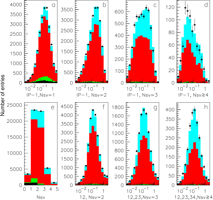
Figure 3: Fit results on a log scale. The stacked MC histograms are from bottom to top: $udsc$ background, $0D$, $1D$, and $2D$. (a)-(d) show the IP to vertex 1 separation [cm], (f)-(h) shows the nearest neighbor vertex separations [cm], and (e) shows the resulting match in the vertex count distribution.

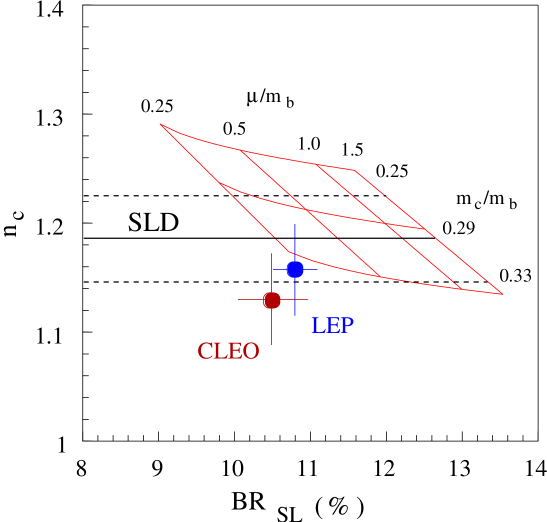
Figure 4: The SLD measurement of $N_{c}$ compared with measurements of $N_{c}$ and $BR_{SL}$ by LEP and CLEO and with theoretical expectations. The new SLD $N_{c}$ result is shown as a horizontal band on this plot.

2 $B$ Mixing

The magnitude of the CKM matrix element $V_{td}$ may be extracted from measurements of the mixing frequencies $\Delta m_{d}$ and $\Delta m_{s}$. The ingredients of the mixing analyses include 1) a selection of neutral $B$ decays from the $B$-tagged sample described above; 2) an initial state flavor tag and 3) a final state flavor tag in order to determine whether a $B$ has mixed before decaying; and 4) a decay length and boost measurement to yield the proper time of the decay. For $\Delta m_{s}$, the mixing frequencies are then measured by performing amplitude fits on the plots of the mixed fraction as a function of proper time to extract the amplitude of each Fourier mode. A likelihood fit to the mixed fraction plot is used to extract $\Delta m_{d}$. Here we report the results of four analyses, three for $\Delta m_{s}$ and one for $\Delta m_{d}$. More information may be found elsewhere$\!{}^{{\bf?}}$ $\!{}^{{\bf?}}$ $\!{}^{{\bf?}}$.

All four analyses share the same techniques for obtaining the neutral $B$ sample, for doing the initial state tag, and for measuring the $B$ boost. The charge of the decaying $B$ is measured by associating charged tracks with a reconstructed $B$ decay vertex to compute the net vertex charge. Selecting the zero charge bin yields a sample which is $87\%$ true neutral decays.

The initial state flavor tag is naturally provided by forward-backward asymmetry in the $Z^{0}$ decay due to the $73\%$ polarization of the SLC $e^{-}$ beam. Other opposite hemisphere information such as the vertex charge, the momentum weighted jet charge, the charges of identified kaons and/or high $P_{t}$ leptons, and the dipole charge (see below), are also used in a neural network optimized tag to achieve a mistag rate of only $22\%$.

The $B$ boost is measured using a combination of calorimetry and of the kinematics of the reconstructed $B$ vertex. $\sigma_{p}/p\approx 0.08$ for the $60\%$ Gaussian core resolution, and $\approx 0.20$ for the tail resolution.

The techniques for the final state tag and decay length measurement are described below. For $\Delta m_{s}$ the analyses are prioritized in the order below from highest to lowest sensitivity. Each $B$ decay is assigned to the highest sensitivty analysis that it qualifies for.

Table 1: Comparison of $\Delta m_{s}$ analyses in the number of events assigned to each analysis, the core and tail decay length resolution, the $B_{s}$ fraction in each event sample, and the final state mistag rate $w$.

	events	$\sigma_{L}(\mu{\rm m})$	$B_{s}$ fraction	w
		core (tail)
Charge Dipole	11462	81 (297)	$16\%$	$22\%$
Lepton + $D$	2087	54 (213)	$16\%$	$4\%$
$D_{s}^{\pm}$ + Tracks	361	50 (151)	$38\%$	$10\%$

2.1 The $\Delta m_{s}$ Analyses

This ‘$D_{s}^{\pm}$ + Tracks’ method utilizes a fully reconstructed $D_{s}^{\pm}$ decay to identify the sign of the $b$ quark. Requiring a $D_{s}^{\pm}$ in the event enhances the $B_{s}$ fraction by rejecting many of the $B_{d}$ decays. The reconstructed $D_{s}^{\pm}$ trajectory is intersected with the remaining tracks from the $B$ decay to get a precise decay length measurement. Because of resulting precise proper time resolution, this method contributes the most analyzing power at large $\Delta m_{s}$ despite having low statistics.

The ‘Lepton+$D$’ method uses a high-$P_{t}$ identified lepton from the $B$ decay to very cleanly identify the sign of the $b$ quark. Selecting semileptonic decays rejects the decays with a wrong-sign $D_{s}^{\pm}$ which dilute the tag purity of the other two analyses. The lepton trajectory is intersected with the inferred trajectory of a reconstructed $D$ vertex in the event to measure the $B$ decay length.

The most inclusive analysis uses the ‘Charge Dipole’ technique which exploits the naturally occurring charge dipole in the $B_{s}\rightarrow D_{s}^{-}X^{+}$ decay cascade. In hemispheres with both the $B$ and the $D$ vertex reconstructed, the charge dipole may be defined as the charge difference ($Q_{D}-Q_{B}$) between the two vertices multiplied by the vertex separation distance. $B_{s}$ ($\bar{B}_{s}$) decays will tend to have negative (positive) values of this quantity. The proper time is then measured from the decay length, defined as the distance between the IP and the closest secondary vertex.

The results of these three analyses are combined to form the amplitude fit plot shown in figure 6. Based on this plot, a lower bound of $\Delta m_{s}<11.1{\rm ps}^{-1}$ at $95\%$ confidence level is calculated. This bound gives an upper bound on $|V_{td}|$ in the $\rho-\eta$ plane of the CKM matrix.

2.2 The $\Delta m_{d}$ Analysis

This analysis tags the sign of the $b$ quark using the identified $K^{\pm}$ from the cascade $D$ decay. This tag is calibrated with the data by simultaneously fitting for $\Delta m_{d}$ and the ‘right sign fraction’ in the $B$ decay sample (figure 6). The latter fraction is measured to be $(79.7\pm 2.2)\%$ of the sample of 7844 $B$ decays used. The mixing frequency is measured to be $\Delta m_{d}=0.503\pm 0.028\pm 0.020$.

Figure 5: $\Delta m_{d}$ likelihood fit to the mixed fraction vs. proper time.

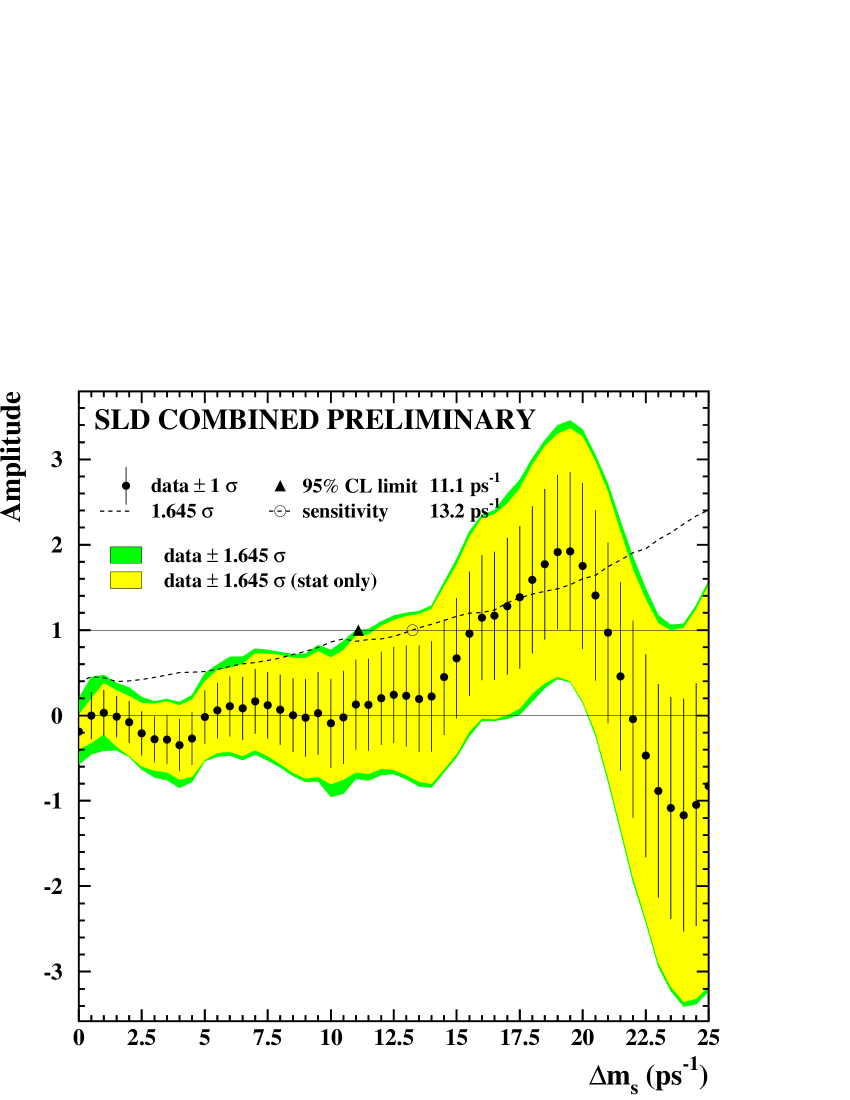
Figure 6: Combined amplitude fit results for $\Delta m_{s}$.

References

References

- [1] M. Neubert and C. T. Sachrajda Nucl. Phys. B483 (1997) 339–370, hep-ph/9603202.
- [2] H. Yamamoto hep-ph/9912308.
- [3] ALEPH, CDF, DELPHI, L3, OPAL, SLD, CERN-EP/2001-050.
- [4] SLD Collaboration, T. Wright et al. SLAC-PUB-8721.
- [5] SLD Collaboration, K. Abe et al. hep-ex/0012043.
- [6] A. S. Chou tech. rep., SLAC, 2001. SLAC-R-578.
- [7] G. Buchalla, I. Dunietz, and H. Yamamoto Phys. Lett. B364 (1995) 188–194, hep-ph/9507437.
- [8] SLD Collaboration, K. Abe et al. hep-ex/0011041.
- [9] J. L. Wittlin tech. rep., SLAC, 2001. SLAC-R-582.