Measurements of Lifetimes, Mixing and $C\!P$ Violation of B Mesons with the BABAR Detector

Using a data sample of 62 million $\mathchar 28935\relax{(4S)}\rightarrow B\kern 1.43994pt\overline{\kern-1.43994ptB}{}$ decays collected between 1999 and 2001 by the BABAR detector at the PEP-II asymmetric-energy $B$ Factory at SLAC we study events in which one neutral $B$ meson is fully reconstructed in a final state containing a charmonium meson and the flavour of the other neutral $B$ meson is determined from its decay products. The amplitude of the $C\!P$-violating asymmetry, which in the Standard Model is proportional to $\sin\!2\beta$, is derived from the decay time distributions. We measure $\sin\!2\beta=0.75\pm 0.09\ \mathrm{(stat)}\pm 0.04\ \mathrm{(syst)}$ and $|\lambda|=0.92\pm 0.06\ \mathrm{(stat)}\pm 0.02\ \mathrm{(syst)}$. The latter is consistent with the Standard Model expectation of no direct $C\!P$ violation. These results are preliminary. In addition, we report on precision measurements of the $B$ lifetimes, and the $B^{0}$-$\kern 1.43994pt\overline{\kern-1.43994ptB}{}^{0}$ oscillation frequency ${\rm\Delta}m_{d}$.

1 Introduction

$C\!P$ violation has been a central concern of particle physics since its discovery in 1964 in the decays of $K^{0}_{\scriptscriptstyle L}$ decays$\!{}^{{\bf?}}$. An elegant explanation of the $C\!P$-violating effects in these decays is provided by the $C\!P$-violating phase of the three-generation Cabibbo-Kobayashi-Maskawa (CKM) quark-mixing matrix $\!{}^{{\bf?}}$. However, existing studies of $C\!P$ violation in neutral kaon decays and the resulting experimental constraints on the parameters of the CKM matrix $\!{}^{{\bf?}}$ do not provide a stringent test of whether the CKM phase describes $C\!P$ violation $\!{}^{{\bf?}}$. In the CKM picture, large $C\!P$ violating asymmetries are expected in the time distributions of $B^{0}$ decays to charmonium final states.

In general, $C\!P$ violating asymmetries are due to the interference between amplitudes with a weak phase difference. For example, a state initially produced as a $B^{0}$ ($\kern 1.79993pt\overline{\kern-1.79993ptB}{}^{0}$) can decay to a $C\!P$ eigenstate such as ${J\mskip-3.0mu/\mskip-2.0mu\psi\mskip 2.0mu}K^{0}_{\scriptscriptstyle S}$ directly or can oscillate into a $\kern 1.79993pt\overline{\kern-1.79993ptB}{}^{0}$ ($B^{0}$) and then decay to ${J\mskip-3.0mu/\mskip-2.0mu\psi\mskip 2.0mu}K^{0}_{\scriptscriptstyle S}$. With little theoretical uncertainty in the Standard Model, the phase difference between these amplitudes is equal to twice the angle $\beta=\arg\left[\,-V_{\rm cd}V_{\rm cb}^{*}/V_{\rm td}V_{\rm tb}^{*}\,\right]$ of the Unitarity Triangle. The $C\!P$-violating asymmetry in this mode allows a direct determination of $\sin\!2\beta$, and can thus provide a crucial test of the Standard Model.

A $B^{0}{\kern-1.60004pt\kern 1.79993pt\overline{\kern-1.79993ptB}{}^{0}}$ pair produced in $\mathchar 28935\relax{(4S)}$ decays evolves in a coherent $P$-wave until one of the $B$ mesons decays. If one of the $B$ mesons, referred to as $B_{\rm tag}$, can be ascertained to decay to a state of known flavour, i.e. $B^{0}$ or $\kern 1.79993pt\overline{\kern-1.79993ptB}{}^{0}$, at a certain time $t_{\rm tag}$, the other $B$, referred to as $B_{\rm rec}$, at that time must be of the opposite flavour as a consequence of Bose symmetry. Consequently, the oscillatory probabilities for observing $B^{0}{\kern-1.60004pt\kern 1.79993pt\overline{\kern-1.79993ptB}{}^{0}}$, $B^{0}B^{0}$ and $\kern 1.79993pt\overline{\kern-1.79993ptB}{}^{0}\kern 1.79993pt\overline{\kern-1.79993ptB}{}^{0}$ pairs produced in $\mathchar 28935\relax{(4S)}$ decays are a function of ${\rm\Delta}t=t_{\rm rec}-t_{\rm tag}$, allowing mixing frequency and $C\!P$ asymmetries to be determined if ${\rm\Delta}t$ is known.

At the PEP-II asymmetric $e^{+}e^{-}$ collider $\!{}^{{\bf?}}$, resonant production of the $\mathchar 28935\relax{(4S)}$  provides a copious source of $B^{0}{\kern-1.60004pt\kern 1.79993pt\overline{\kern-1.79993ptB}{}^{0}}$ pairs moving along the beam axis ($z$ direction) with an average Lorentz boost of $\left<\beta\gamma\right>=0.55$. Therefore, the proper decay-time difference ${\rm\Delta}t$ is, to an excellent approximation, proportional to the distance ${\rm\Delta}z$ between the two $B^{0}$-decay vertices along the axis of the boost, ${\rm\Delta}t\approx{\rm\Delta}z/c\left<\beta\gamma\right>$. The average separation between the two $B$ decay vertices is ${\rm\Delta}z\approx\left<\beta\gamma\right>c\tau_{B}=260$$\,\mu\rm m$, while the RMS ${\rm\Delta}z$ resolution of the detector is about 180$\,\mu\rm m$.

The lifetime, mixing and $\sin\!2\beta$ analyses share a common analysis strategy:

• select events where one $B$, labeled $B_{\rm rec}$, is fully reconstructed;

• determine the vertex of the other $B$ decay, $B_{\rm tag}$, in the event by performing a vertex fit to the remaining charged particle trajectories, and compute ${\rm\Delta}t$.

At this point, one can perform an unbinned likelihood fit to the ${\rm\Delta}t$ distribution and determine the $B$ lifetime. The mixing and $C\!P$  asymmetry measurements require one additional step:

• determine the flavour of the $B_{\rm tag}$ decay.

To determine the oscillation frequency ${\rm\Delta}m_{d}$   events are selected where $B_{\rm rec}$ is reconstructed in a neutral decay mode with a known flavour, such as $D^{*+}\pi^{-}$, and a simultaneous unbinned likelihood fit to the ${\rm\Delta}t$ distributions of events where $B_{\rm rec}$ and $B_{\rm tag}$ have opposite flavour (unmixed) and equal flavour (mixed) is performed. To determine $C\!P$ asymmetries, $B_{\rm rec}$ is a reconstructed $C\!P$ final state such as ${J\mskip-3.0mu/\mskip-2.0mu\psi\mskip 2.0mu}K^{0}_{\scriptscriptstyle S}$, and the ${\rm\Delta}t$ distributions of events where $B_{\rm tag}$ is a $B^{0}$ and $\kern 1.79993pt\overline{\kern-1.79993ptB}{}^{0}$ respectively are fitted simultaneously.

In order to establish the experimental technique, we first present precision measurements of the $B^{0}$ and $B^{+}$ lifetimes, and the $B^{0}$ $\kern 1.79993pt\overline{\kern-1.79993ptB}{}^{0}$ oscillation frequency ${\rm\Delta}m_{d}$. These measurements share the same vertexing algorithm and ${\rm\Delta}t$ determination as the measurement of the $C\!P$ asymmetries, and, in case of the mixing measurement, the same flavour tagging algorithm. To eliminate possible experimenter’s bias the parameter under study was hidden in all analyses until the event selection and reconstruction, fitting procedure and systematic errors were finalized.

2 The BABAR detector and data sets

The data used were recorded with the BABAR detector in the period October 1999–December 2001. The total integrated luminosity of the data set is equivalent to 56$\mbox{\,fb}^{-1}$ collected near the $\mathchar 28935\relax{(4S)}$ resonance. The corresponding number of produced $B\kern 1.79993pt\overline{\kern-1.79993ptB}{}$ pairs is estimated to be about 62 million. The measurement of the charged and neutral $B$ lifetimes is based on the initial 23 million $B\kern 1.79993pt\overline{\kern-1.79993ptB}{}$ pairs, whereas the dataset used for the ${\rm\Delta}m_{d}$ measurement includes the first 32 million $B\kern 1.79993pt\overline{\kern-1.79993ptB}{}$ pairs. This latter sample was also used for the previously published measurement$\!{}^{{\bf?}}$ of $\sin\!2\beta$; in contrast, the preliminary measurement of $\sin\!2\beta$ described here utilizes the entire data sample available.

Since the BABAR detector is described in detail elsewhere $\!{}^{{\bf?}}$, only a brief description is given here. Surrounding the beam-pipe is a 5-layer silicon vertex tracker (SVT), which provides precise measurements of the trajectories of charged particles as they leave the $e^{+}e^{-}$ interaction point. Outside of the SVT, a 40-layer drift chamber (DCH) allows measurements of track momenta in a 1.5 T magnetic field as well as energy-loss measurements, which contribute to charged particle identification. Surrounding the DCH is a detector of internally reflected Cherenkov radiation (DIRC), which provides charged hadron identification. Outside of the DIRC is a CsI(Tl) electromagnetic calorimeter (EMC) that is used to detect photons, provide electron identification and reconstruct neutral hadrons. The EMC is surrounded by a superconducting coil, which creates the magnetic field for momentum measurements. Outside of the coil, the flux return is instrumented with resistive plate chambers interspersed with iron (IFR) for the identification of muons and long-lived neutral hadrons. We use the GEANT4 package $\!{}^{{\bf?}}$ to simulate interactions of particles traversing the BABAR detector.

3 Measurement of $B$ Lifetimes and ${\rm\Delta}m_{d}$

3.1 Exclusive $B$ reconstruction

The so-called $B_{\rm{flav}}$ sample used for lifetime and mixing analyses consists of events where $B_{\rm rec}$ is reconstructed in the modes $B^{0}\rightarrow D^{(*)-}\pi^{+}$, $D^{(*)-}\rho^{+}$, $D^{(*)-}a_{1}^{+}$, ${J\mskip-3.0mu/\mskip-2.0mu\psi\mskip 2.0mu}K^{*0}$ and $B^{+}\rightarrow\kern 1.99997pt\overline{\kern-1.99997ptD}{}^{(*)0}\pi^{+}$, ${J\mskip-3.0mu/\mskip-2.0mu\psi\mskip 2.0mu}K^{+}$, $\psi{(2S)}K^{+}$. Charged and neutral $\kern 1.99997pt\overline{\kern-1.99997ptD}{}^{*}$ candidates are formed by combining a $\kern 1.99997pt\overline{\kern-1.99997ptD}{}^{0}$ with a $\pi^{-}$ or $\pi^{0}$. $\kern 1.99997pt\overline{\kern-1.99997ptD}{}^{0}$ candidates are reconstructed in the decay channels $K^{+}\pi^{-}$, $K^{+}\pi^{-}\pi^{0}$, $K^{+}\pi^{+}\pi^{-}\pi^{-}$ and $K^{0}_{\scriptscriptstyle S}\pi^{+}\pi^{-}$ and $D^{-}$ candidates in the decay channels $K^{+}\pi^{-}\pi^{-}$ and $K^{0}_{\scriptscriptstyle S}\pi^{-}$. We reconstruct ${J\mskip-3.0mu/\mskip-2.0mu\psi\mskip 2.0mu}$ and $\psi{(2S)}$ in the decays to $e^{+}e^{-}$ and $\mu^{+}\mu^{-}$ and the $\psi{(2S)}$ decay to ${J\mskip-3.0mu/\mskip-2.0mu\psi\mskip 2.0mu}$ $\pi^{+}$ $\pi^{-}$.

Continuum $e^{+}e^{-}\rightarrow q\overline{q}$ background is suppressed by requirements on the normalized second Fox-Wolfram moment $\!{}^{{\bf?}}$ for the event and on the angle between the thrust axes of $B_{\rm rec}$ and of the other $B$ in the event. $B_{\rm rec}$ candidates are identified by the difference $\Delta\rm{E}$ between the reconstructed $B$ energy and $\sqrt{s}/2$ in the $\mathchar 28935\relax{(4S)}$ frame, and the beam-energy substituted mass $m_{\rm ES}$ calculated from $\sqrt{s}/2$ and the reconstructed $B$ momentum. We require $\mbox{$m_{\rm ES}$}>5.2$${\mathrm{\,Ge\kern-1.00006ptV\!/}c^{2}}$ and $|\Delta\rm{E}|<3\sigma_{\Delta\rm{E}}$. The distributions of $m_{\rm ES}$ for selected $B_{\rm{flav}}$ candidates is shown in Fig. 1.

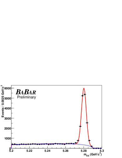
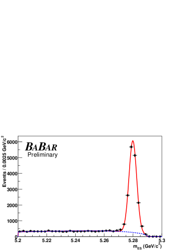
Figure 1: Beam energy substituted mass distribution for selected $B^{0}$ (a) and $B^{+}$ (b) candidates. In 56 $\mbox{\,fb}^{-1}$, we reconstruct 15K $B^{0}$ and 13K $B^{+}$ flavour tagged signal events. Average signal purities for $\mbox{$m_{\rm ES}$}>5.27{\mathrm{\,Ge\kern-1.00006ptV\!/}c^{2}}$, are 85 % and 89 %, respectively.

3.2 ${\rm\Delta}t$ determination

The decay time difference, ${\rm\Delta}t$, between the two $B$ decays is determined from the measured separation, $\Delta z=z_{rec}-z_{tag}$, along the $z$ axis between the reconstructed $\mbox{$B_{\rm rec}$}(z_{rec})$ and flavour-tagging decay $B_{\rm tag}$ vertex $(z_{tag})$. This measured $\Delta z$ is converted into ${\rm\Delta}t$ with the known $\mathchar 28935\relax{(4S)}$ boost, including a correction on an event-by-event basis for the direction of the $B$ mesons with respect to the $z$ direction in the $\mathchar 28935\relax{(4S)}$ frame. The ${\rm\Delta}t$ resolution is limited by the $z$ resolution of the tagging vertex. The $B_{\rm tag}$ decay vertex reconstruction starts from all tracks in the event except those incorporated in $B_{rec}$. An additional constraint is provided by the calculated $B_{\rm tag}$ production point and three-momentum, determined from the three-momentum of the fully reconstructed $B_{\rm rec}$ candidate, its decay vertex, and the average position of the interaction point (with a vertical size of 10$\,\mu\rm m$) and the $\mathchar 28935\relax{(4S)}$ average boost. The derived $B_{\rm tag}$ trajectory is fit to a common vertex with the remaining tracks in the event. Reconstructed $K^{0}_{\scriptscriptstyle S}$ or $\mathchar 28931\relax$ candidates are used as input to the fit in place of their daughters in order to reduce bias due to long-lived particles. Tracks with a large contribution to the $\chi^{2}$ are iteratively removed from the fit until all remaining tracks have a reasonable fit probability or all tracks are removed. For 99.5% of the reconstructed events the r.m.s ${\rm\Delta}z$ resolution is 180 $\,\mu\rm m$.

Two different parameterizations are used to model the decay-time difference resolution. In the measurements of ${\rm\Delta}m_{d}$ and $\sin\!2\beta$, the time resolution function is approximated by a sum of three Gaussian distributions (core, tail, and outlier) with different means and widths,

$${\cal{R}}(\delta_{\rm t},\sigma_{{\rm\Delta}t};\hat{a}=\{f_{k},S_{k},b_{k},\sigma_{3}\})=\sum_{k=1}^{2}{\frac{f_{k}}{S_{k}\sigma_{{\rm\Delta}t}\sqrt{2\pi}}\,{\rm exp}\left(-\frac{(\delta_{\rm t}-b_{k}\sigma_{{\rm\Delta}t})^{2}}{2({S_{k}\sigma_{{\rm\Delta}t}})^{2}}\right)}+{\frac{f_{3}}{\sigma_{3}\sqrt{2\pi}}\,{\rm exp}\left(-\frac{\delta_{\rm t}^{2}}{2{\sigma_{3}}^{2}}\right)},$$

where $\delta_{\rm t}={\rm\Delta}t-{\rm\Delta}t_{\rm true}$. For the core and tail Gaussians, the widths $\sigma_{k}=S_{k}\times\sigma_{{\rm\Delta}t}$ are the event-by-event measurement errors scaled by a common factor $S_{k}$. The scale factor of the tail Gaussian is fixed to the Monte Carlo value since it is strongly correlated with the other resolution function parameters. The third Gaussian, with a fixed width of $\sigma_{3}=8$${\rm\,ps}$, accounts for outlier events with incorrectly reconstructed vertices (less than 1% of events). The offsets $b_{i}$ are modeled to be proportional to $\sigma_{{\rm\Delta}t}$, which is correlated with the weight that the remaining daughters of charm particles have in the tag vertex reconstruction. The tail and outlier fractions and the scale factors are assumed to be the same for all decay modes, since the precision of the $B_{\rm tag}$ vertex measurement is the limiting factor for the ${\rm\Delta}t$ resolution. This assumption is confirmed by Monte Carlo studies.

The three Gaussian resolution function is less suited for the measurements of $B$ lifetimes due to the large correlation between the resolution function parameters and the lifetimes, which leads to increased statistical errors. Studies with Monte Carlo simulations and data show that the sum of a zero-mean Gaussian distribution and its convolution with a one-sided exponential provides a good trade-off between statistical and systematic uncertainties in the lifetime measurement:

$${\cal R}(\delta_{t},\sigma_{{\rm\Delta}t}|\hat{a}=\{f_{1},s,\kappa\})=f_{1}\frac{1}{\sqrt{2\pi}s\sigma_{{\rm\Delta}t}}\exp\left(-\frac{\delta_{t}^{2}}{2s^{2}\sigma_{{\rm\Delta}t}^{2}}\right)\ \ \ \ \ \ \ \ \ \ \ \ \$$ (1)

$$+\int_{-\infty}^{0}\frac{1-f_{1}}{\kappa\sigma_{{\rm\Delta}t}}\exp\left(\frac{\delta_{t}^{\prime}}{\kappa\sigma_{{\rm\Delta}t}}\right)\frac{1}{\sqrt{2\pi}s\sigma_{{\rm\Delta}t}}\exp\left(-\frac{(\delta_{t}-\delta_{t}^{\prime})^{2}}{2s^{2}\sigma_{{\rm\Delta}t}^{2}}\right){\rm d}(\delta_{t}^{\prime})\;.$$

The parameters $\hat{a}$ are the fraction $f$ in the core Gaussian component, a scale factor $s$ for the per-event errors $\sigma_{{\rm\Delta}t}$, and the factor $\kappa$ in the effective time constant $\kappa\sigma_{{\rm\Delta}t}$ of the exponential which accounts for charm decays. $\Delta t$ outlier events are modeled the same way as in the three Gaussian resolution function. The resolution functions differ only slightly between $B^{0}$ and $B^{+}$ mesons due to different mixtures of $D^{-}$ and $\kern 1.99997pt\overline{\kern-1.99997ptD}{}^{0}$  mesons in the $B_{\rm tag}$ decays and we use a single set of resolution function parameters for both $B^{0}$ and $B^{+}$ in the lifetime fits.

3.3 Lifetime results

We extract the $B^{+}$ and $B^{0}$ lifetimes from an unbinned maximum likelihood fit to the ${\rm\Delta}t$ distributions of the selected $B$ candidates. The probability for an event to be signal is estimated from $m_{\rm ES}$ fits (Fig. 1) and the $m_{\rm ES}$ value of the $B_{\rm rec}$ candidate. In the likelihood, the probability density for the signal events is given by

$${\cal G}({\rm\Delta}t,\sigma_{{\rm\Delta}t}|\tau,\hat{a})=\int_{-\infty}^{+\infty}e^{-|{\rm\Delta}t|/\tau}/(2\tau)\,{\cal R}\it({\rm\Delta}t-{\rm\Delta}t^{\prime},\sigma_{{\rm\Delta}t}|\hat{a})\;{\rm d}({\rm\Delta}t^{\prime}),$$ (2)

and the background ${\rm\Delta}t$ distribution for each $B$ species is empirically modeled by the sum of a prompt component and a lifetime component convolved with the same resolution function, but with a separate set of parameters. The likelihood fit involves 17 free parameters in addition to the $B^{0}$ and the $B^{+}$ lifetimes: 12 to describe the background ${\rm\Delta}t$ distributions and 5 for the signal resolution function. The charged $B$ lifetime $\tau_{B^{+}}$ is replaced with $\tau_{B^{+}}=r\cdot\tau_{B^{0}}$ to estimate the statistical error on the ratio $r=\tau_{B^{+}}/\tau_{B^{0}}$.

We determine the $B^{0}$ and $B^{+}$ meson lifetimes and their ratio to be:

$$\tau_{B^{0}} = 1.546\pm 0.032\mbox{ $\mathrm{(stat)}$}\pm 0.022\mbox{ $\mathrm{(syst)}$}\mbox{ ps,}$$

$$\tau_{B^{+}} = 1.673\pm 0.032\mbox{ $\mathrm{(stat)}$}\pm 0.023\mbox{ $\mathrm{(syst)}$}\mbox{ ps, and}$$

$$\tau_{B^{+}}/\tau_{B^{0}} = 1.082\pm 0.026\mbox{ $\mathrm{(stat)}$}\pm 0.012\mbox{ $\mathrm{(syst)}$}.$$

These are the most precise published measurements to date $\!{}^{{\bf?}}$ and are consistent with the world averages $\!{}^{{\bf?}}$. The resolution function parameters are consistent with those found in a Monte Carlo simulation that includes detector alignment effects. With the current data sample these measurements are still statistically limited. The dominant systematic errors arise from uncertainties in the description of the combinatorial background and of events with large ${\rm\Delta}t$ values, the use of a common time resolution function for $B^{0}$ and $B^{+}$ and from limited Monte Carlo statistics.

3.4 Flavour tagging

After the daughter tracks of the $B_{\rm rec}$ are removed from the event, the remaining tracks are analyzed to determine the flavour of the $B_{\rm tag}$, and this ensemble is assigned a tag flavour, either $B^{0}$ or $\kern 1.79993pt\overline{\kern-1.79993ptB}{}^{0}$. For this purpose, flavour tagging information carried by primary leptons from semileptonic $B$ decays, charged kaons, soft pions from $D^{*}$ decays, and more generally by high momentum charged particles is used to uniquely assign an event to a tagging category.

Events are assigned a Lepton tag if they contain an identified lepton with a center-of-mass momentum greater than 1.0 or 1.1${\mathrm{\,Ge\kern-1.00006ptV\!/}c}$ for electrons and muons, respectively. The momentum requirement selects mostly primary leptons by suppressing opposite-sign leptons from semileptonic charm decays. If the sum of charges of all identified kaons is non-zero, the event is assigned a Kaon tag. The final two tags involve a multi-variable analysis based on a neural network, which is trained to identify primary leptons, kaons, and soft pions, and the momentum and charge of the track with the maximum center-of-mass momentum. Depending on the output of the neural net, events are assigned either an NT1 (more certain) tag, an NT2 (less certain) tag, or are considered not tagged (about 30% of events) and excluded from the analysis. The tagging power of the NT1 and NT2 tags comes primarily from slow pions, from kinematically recovering non-identified primary electrons and muons, and from kaons that do not pass the selection criteria for the Kaon category.

Tagging assignments are made mutually exclusive by the hierarchical use of the tags. Events with a Lepton tag and no conflicting Kaon tag are assigned to the Lepton category. If no Lepton tag exists, but the event has a Kaon tag, it is assigned to the Kaon category. Otherwise the event is assigned to one of the two neural network categories.

The effective tagging efficiency $Q_{i}=\varepsilon_{i}(1-2w_{i})^{2}$, where $\varepsilon_{i}$ is the fraction of events assigned to category $i$ and $w_{i}$ the probability of obtaining a wrong tag, is used as the basis for optimization of category selection criteria. The statistical errors on ${\rm\Delta}m_{d}$ and $\sin\!2\beta$ are proportional to $1/\sqrt{Q}$, where $Q=\sum{Q_{i}}$. The contributions of the various tagging categories to $Q$ is shown in Table 1.

Table 1: Tagging efficiency $\varepsilon$, average mistag fractions $w$, mistag differences $\Delta w=w(B^{0})-w(\kern 1.79993pt\overline{\kern-1.79993ptB}{}^{0})$, and the derived $Q$ (defined in the text) obtained from the likelihood fit to the $B_{\rm{flav}}$ and $B_{C\!P}$ samples.

Category	$\ \ \ \varepsilon$ (%)	$\ \ \ w$ (%)	$\ \ \ \Delta w$ (%)	$\ \ \ Q$ (%)
Lepton	$11.1\ \pm\ 0.2$	$8.6\ \pm\ 0.9$	$0.6\ \pm\ 1.5$	$7.6\ \pm\ 0.4$
Kaon	$34.7\ \pm\ 0.4$	$18.1\ \pm\ 0.7$	$-0.9\ \pm\ 1.1$	$14.1\ \pm\ 0.6$
NT1	$~{}7.7\ \pm\ 0.2$	$22.0\ \pm\ 1.5$	$1.4\ \pm\ 2.3$	$2.4\ \pm\ 0.3$
NT2	$14.0\ \pm\ 0.3$	$37.3\ \pm\ 1.3$	$-4.7\ \pm\ 1.9$	$0.9\ \pm\ 0.2$
All	$67.5\ \pm\ 0.5$			$25.1\ \pm\ 0.8$

3.5 Mixing result

The value of ${\rm\Delta}m_{d}$ is extracted from the tagged flavour-eigenstate $B^{0}$ sample with a simultaneous unbinned likelihood fit to the ${\rm\Delta}t$ distributions of both unmixed and mixed events. The PDFs for the unmixed $(+)$ and mixed $(-)$ signal events for the $i^{th}$ tagging category are given by

$${\cal H}_{\pm}({\rm\Delta}t,\sigma_{{\rm\Delta}t}|{\rm\Delta}m_{d},w_{i},\hat{a}_{i})=\frac{{\rm e}^{-\left|{\rm\Delta}t\right|/\tau}}{4\tau}\left[1\pm(1-2w_{i})\cos{{\rm\Delta}m_{d}{\rm\Delta}t}\right]\otimes{\cal R}(\delta_{t},\sigma_{{\rm\Delta}t}|\hat{a}_{i}).$$ (3)

Some resolution function parameters are allowed to differ for each tagging category to account for shifts due to inclusion of charm decay products in the tag vertex. The PDFs are extended to include background terms, different for each tagging category. The probability that a $B^{0}$ candidate is a signal event is determined from a fit to the observed $m_{\rm ES}$ distribution for its tagging category. The ${\rm\Delta}t$ distributions of the combinatorial background are described with a zero lifetime component and a non-oscillatory component with non-zero lifetime. Separate resolution function parameters are used for signal and background to minimize correlations.

The $\Delta t$ distributions of the signal ($\mbox{$m_{\rm ES}$}>5.27{\mathrm{\,Ge\kern-1.00006ptV\!/}c^{2}}$) overlaid with the projections of the likelihood fit, are shown in Fig. 2. In addition, the mixing asymmetry,

$${\cal A}_{mix}({\rm\Delta}t)=\frac{N_{unmixed}({\rm\Delta}t)-N_{mixed}({\rm\Delta}t)}{N_{unmixed}({\rm\Delta}t)+N_{mixed}({\rm\Delta}t)}.$$ (4)

is plotted. If flavour tagging and ${\rm\Delta}t$ determination were perfect, the asymmetry as a function of ${\rm\Delta}t$ would be a cosine with unit amplitude.

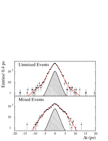
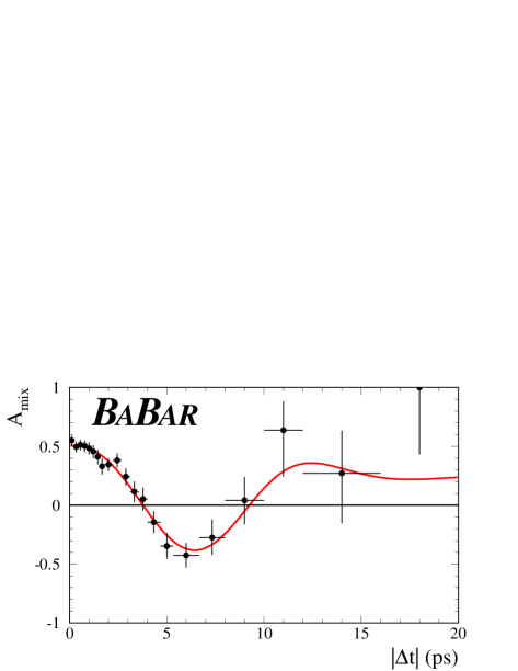
Figure 2: Distributions of ${\rm\Delta}t$ for (a) unmixed and (b) mixed events in the signal region $\mbox{$m_{\rm ES}$}>5.27$${\mathrm{\,Ge\kern-1.00006ptV\!/}c^{2}}$. The data points are overlaid with the result from the fit, projected using the individual signal probabilities and event-by-event ${\rm\Delta}t$ resolutions, along with the simultaneously determined background distribution. Also shown (c) is the time-dependent mixing asymmetry ${\cal A}_{mix}(|{\rm\Delta}t|)$ defined in the text.

The probability to obtain a likelihood smaller than that observed is 44%, evaluated with a parameterized Monte Carlo technique. The value of ${\rm\Delta}m_{d}$ obtained is

$${\rm\Delta}m_{d}=0.516\pm 0.016({stat})\pm 0.010({syst})\,\mbox{${\rm\,ps}^{-1}$}.$$ (5)

Since the parameters of the ${\rm\Delta}t$ resolution and the mistag rates $w$ are free parameters in the fit, their contribution to the uncertainty on ${\rm\Delta}m_{d}$ is included as part of the statistical error. The main contributions to the systematic errors are the choice of the signal ${\rm\Delta}t$ resolution description, its capability to handle outliers and various worst-case SVT misalignment scenarios ($\pm 0.005\mbox{${\rm\,ps}^{-1}$}$), and by correlations between mistag rates and ${\rm\Delta}t$ resolution which are not explicitly modeled by the likelihood fit ($\pm 0.005\mbox{${\rm\,ps}^{-1}$}$). Finally, the variation of the fixed $B^{0}$ lifetime within known errors $\!{}^{{\bf?}}$ leads to a systematic uncertainty of $\pm 0.006\mbox{${\rm\,ps}^{-1}$}$.

This is one of the single most precise mixing measurements available$\!{}^{{\bf?}}$, and is consistent with the current world average $\!{}^{{\bf?}}$.

4 Determination of $\sin\!2\beta$

For the measurement of $\sin\!2\beta$, $B_{\rm rec}$ is fully reconstructed in a $C\!P$ eigenstate with eigenvalue $\eta_{C\!P}=-1$ (${J\mskip-3.0mu/\mskip-2.0mu\psi\mskip 2.0mu}K^{0}_{\scriptscriptstyle S}$, $\psi{(2S)}K^{0}_{\scriptscriptstyle S}$, or $\chi_{c1}K^{0}_{\scriptscriptstyle S}$) or $+1$ (${J\mskip-3.0mu/\mskip-2.0mu\psi\mskip 2.0mu}K^{0}_{\scriptscriptstyle L}$), while $B_{\rm tag}$ is tagged just as for the mixing measurement. The sample is further enlarged by including the mode ${J\mskip-3.0mu/\mskip-2.0mu\psi\mskip 2.0mu}K^{*0}$ ($K^{*0}\rightarrow K^{0}_{\scriptscriptstyle S}\pi^{0}$). However, due to the presence of even ($L=0$, 2) and odd ($L=1$) orbital angular momenta in the ${J\mskip-3.0mu/\mskip-2.0mu\psi\mskip 2.0mu}K^{*0}$ system, there are $\eta_{C\!P}=-1$ and $+1$ contributions to its decay rate. These contributions are disentangled by incorporating their dependence on the transversity angles in each event into the likelihood fit$\!{}^{{\bf?}}$. The $m_{\rm ES}$ distributions ($\Delta\rm{E}$ for ${J\mskip-3.0mu/\mskip-2.0mu\psi\mskip 2.0mu}$ $K^{0}_{\scriptscriptstyle L}$) of the selected sample are shown in Fig. 3, and the detailed breakdown in Table 2.

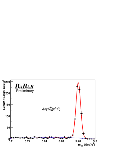
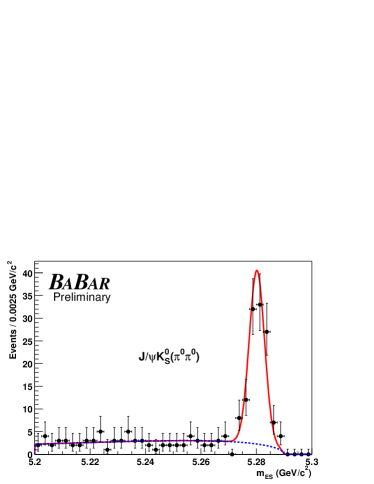
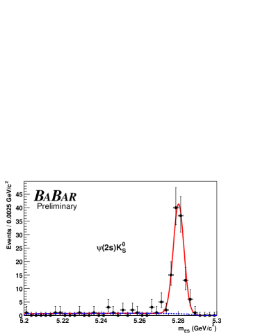
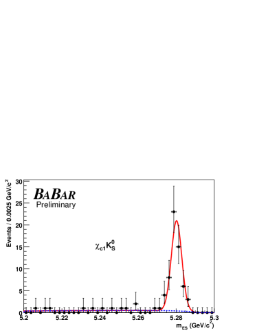
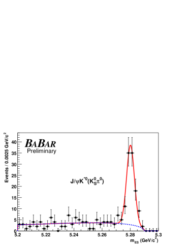
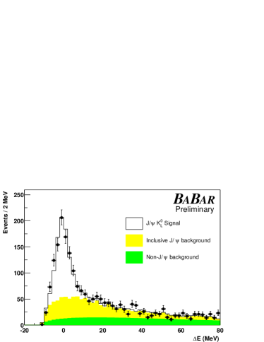
Figure 3: Distribution of $m_{\rm ES}$ for flavour tagged $B_{C\!P}$ candidates selected in the final states a) $J/\psi K^{0}_{S}\ (K^{0}_{\scriptscriptstyle S}\rightarrow\pi^{+}\pi^{-})$, b) $J/\psi K^{0}_{S}\ (K^{0}_{\scriptscriptstyle S}\rightarrow\pi^{0}\pi^{0})$, c) $\psi(2S)K^{0}_{S}$, d) $\chi_{c1}K^{0}_{S}$, e) $J/\psi K^{*0}(K^{*0}\rightarrow K^{0}_{S}\pi^{0})$, and f) distribution of $\Delta E$ for flavour tagged ${J\mskip-3.0mu/\mskip-2.0mu\psi\mskip 2.0mu}K^{0}_{\scriptscriptstyle L}$ candidates.

Table 2: Number of tagged events, signal purity, and result of fitting for $C\!P$ asymmetries in the full $C\!P$ sample and in various subsamples, as well as in the $B_{\rm flav}$ and charged $B$ control samples. Purity is the fitted number of signal events divided by the total number of events in the $\Delta E$ and $m_{\rm ES}$ signal region defined in the text.

Sample	$N_{\rm tag}$	Purity (%)	$\ \ \ \sin\!2\beta$
Full $C\!P$ sample	1850	79	$0.75\ \pm\ 0.09$
$\ {J\mskip-3.0mu/\mskip-2.0mu\psi\mskip 2.0mu}K^{0}_{\scriptscriptstyle S}$ ($K^{0}_{\scriptscriptstyle S}\rightarrow\pi^{+}\pi^{-}$)	693	96	$0.79\ \pm\ 0.11$
$\ {J\mskip-3.0mu/\mskip-2.0mu\psi\mskip 2.0mu}K^{0}_{\scriptscriptstyle S}$ ($K^{0}_{\scriptscriptstyle S}\rightarrow\pi^{0}\pi^{0}$)	123	89	$0.42\ \pm\ 0.33$
$\ \psi(2S)K^{0}_{\scriptscriptstyle S}$	119	89	$0.84\ \pm\ 0.32$
$\ \chi_{c1}K^{0}_{\scriptscriptstyle S}$	60	94	$0.84\ \pm\ 0.49$
$\ {J\mskip-3.0mu/\mskip-2.0mu\psi\mskip 2.0mu}K^{0}_{\scriptscriptstyle L}$	742	57	$0.73\ \pm\ 0.19$
$\ {J\mskip-3.0mu/\mskip-2.0mu\psi\mskip 2.0mu}K^{*0}$ ($K^{*0}\rightarrow K^{0}_{\scriptscriptstyle S}\pi^{0}$)	113	83	$0.62\ \pm\ 0.56$
${J\mskip-3.0mu/\mskip-2.0mu\psi\mskip 2.0mu}K^{0}_{\scriptscriptstyle S}$, $\psi{(2S)}K^{0}_{\scriptscriptstyle S}$, $\chi_{c1}K^{0}_{\scriptscriptstyle S}$ only $(\eta_{f}=-1)$	995	94	$0.76\ \pm\ 0.10$
Lepton tags	176	97	$0.73\ \pm\ 0.16$
Kaon tags	504	95	$0.75\ \pm\ 0.14$
NT1 tags	117	95	$0.86\ \pm\ 0.33$
NT2 tags	198	94	$0.84\ \pm\ 0.61$
$B^{0}$ tags	471	94	$0.79\ \pm\ 0.14$
$\kern 1.79993pt\overline{\kern-1.79993ptB}{}^{0}$ tags	524	95	$0.73\ \pm\ 0.14$
$B_{\rm flav}$ sample	17546	85	$0.00\ \pm\ 0.03$
Charged $B$ sample	14768	89	$-0.02\ \pm\ 0.03$

The decay-time distribution of $B$ decays to a $C\!P$ eigenstate with a $B^{0}$ or $\kern 1.79993pt\overline{\kern-1.79993ptB}{}^{0}$ tag can be expressed in terms of a complex parameter $\lambda$ that depends on both the $B^{0}$-$\kern 1.79993pt\overline{\kern-1.79993ptB}{}^{0}$ oscillation amplitude and the amplitudes describing $\kern 1.79993pt\overline{\kern-1.79993ptB}{}^{0}$ and $B^{0}$ decays to this final state $\!{}^{{\bf?}}$. The decay rate ${\cal F}_{+}({\cal F}_{-})$ when the tagging meson is a $B^{0}(\kern 1.79993pt\overline{\kern-1.79993ptB}{}^{0})$ is given by

$${\cal F}_{\pm}({\rm\Delta}t,\sigma_{{\rm\Delta}t}|\sin\!2\beta,w_{i},\hat{a}_{i})$$ (6)

$$= {\frac{{\rm e}^{{-\left|{\rm\Delta}t\right|}/\tau_{B^{0}}}}{4\tau_{B^{0}}}}\left[\ 1\hbox to0.0pt{}\pm\left(1-2w_{i}\right)\left(\frac{{2\mathop{\cal I\mkern-2.0mu\mit m}}\lambda}{1+|\lambda|^{2}}\sin{({\rm\Delta}m_{d}{\rm\Delta}t)}-{\frac{1-|\lambda|^{2}}{1+|\lambda|^{2}}}\cos{({\rm\Delta}m_{d}{\rm\Delta}t)}\right)\right]$$

$$\otimes {\cal R}(\delta_{t},\sigma_{{\rm\Delta}t}|\hat{a}_{i}),$$

where the $+$ or $-$ sign indicates whether the $B_{\rm tag}$ is tagged as a $B^{0}$ or a $\kern 1.79993pt\overline{\kern-1.79993ptB}{}^{0}$, respectively.

The distributions are much simpler when $|\lambda|=1$, which is the expectation of the Standard Model for decays like $B^{0}\rightarrow{J\mskip-3.0mu/\mskip-2.0mu\psi\mskip 2.0mu}K^{0}_{\scriptscriptstyle S}$ where all amplitudes which contribute to the decay have the same weak phase. In this particular case one is left with the phase difference introduced by $B^{0}$-$\kern 1.79993pt\overline{\kern-1.79993ptB}{}^{0}$ mixing, i.e. $\lambda=\eta_{C\!P}{\rm e}^{2i\beta}$. where $\eta_{C\!P}$ is the $C\!P$ eigenvalue of the final state.

It is possible to construct a $C\!P$-violating observable which, neglecting resolution effects, is proportional to $\sin\!2\beta$:

$${\cal A}_{CP}({\rm\Delta}t)=\frac{{\cal F}_{+}({\rm\Delta}t)-{\cal F}_{-}({\rm\Delta}t)}{{\cal F}_{+}({\rm\Delta}t)+{\cal F}_{-}({\rm\Delta}t)}\propto-\eta_{C\!P}{\left(1-2w\right)}\sin{2\beta}\sin{{\rm\Delta}m_{d}{\rm\Delta}t}.$$ (7)

Since no time-integrated $C\!P$ asymmetry effect is expected, an analysis of the time-dependent asymmetry is necessary. The interference between the two amplitudes, and hence the $C\!P$ asymmetry, is maximal after approximately 2.1 $B^{0}$ proper lifetimes, when the mixing asymmetry goes through zero. However, the maximum sensitivity to $\sin\!2\beta$, which is proportional to ${\rm e}^{-\Gamma{\rm\Delta}t}\sin^{2}{\rm\Delta}m_{d}{\rm\Delta}t$, occurs in the region of 1.4 lifetimes.

The value of $\sin\!2\beta$ can be extracted by maximizing the likelihood function

$$\ln{{\cal{L}}_{CP}}=\sum_{i}^{\rm tagging}\left[\sum_{B^{0}\ {\rm tag}}{\ln{{\cal F}_{+}({\rm\Delta}t,\sigma_{{\rm\Delta}t};\sin\!2\beta,w_{i},\hat{a}_{i},)}}+\sum_{\kern 1.25995pt\overline{\kern-1.25995ptB}{}^{0}\ {\rm tag}}{\ln{{\cal F}_{-}({\rm\Delta}t,\sigma_{{\rm\Delta}t};\sin\!2\beta,w_{i},\hat{a}_{i},)}}\right],$$ (8)

where the outer summation is over tagging categories $i$ and the inner summations are over the $B^{0}$ and $\kern 1.79993pt\overline{\kern-1.79993ptB}{}^{0}$ tags within a given tagging category. In practice, the fit for $\sin\!2\beta$ is performed on the combined $B_{\rm{flav}}$ and $B_{C\!P}$ samples with a likelihood constructed from the sum of Eq. 3 and 8, in order to determine $\sin\!2\beta$, the mistag fraction $w_{i}$ for each tagging category, and the resolution parameters $\hat{a}_{i}$ simultaneously. Additional terms are included in the likelihood to account for backgrounds and their time dependence. The determination of the mistag fractions and ${\rm\Delta}t$ resolution function for the signal is dominated by the high-statistics $B_{\rm{flav}}$ sample. We fix $\tau_{B^{0}}=1.548{\rm\,ps}$ and ${\rm\Delta}m_{d}=0.472{\rm\,ps}^{-1}$ $\!{}^{{\bf?}}$. The largest correlation between $\sin\!2\beta$ and any linear combination of other free parameters is only 0.14.

Figure 4: Number of $\eta_{f}=-1$ candidates ($J/\psi K^{0}_{\scriptscriptstyle S}$, $\psi(2S)K^{0}_{\scriptscriptstyle S}$, $\chi_{c1}K^{0}_{\scriptscriptstyle S}$) in the signal region a) with a $B^{0}$ tag $N_{B^{0}}$ and b) with a $\kern 1.79993pt\overline{\kern-1.79993ptB}{}^{0}$ tag $N_{\kern 1.25995pt\overline{\kern-1.25995ptB}{}^{0}}$, and c) the raw asymmetry $(N_{B^{0}}-N_{\kern 1.25995pt\overline{\kern-1.25995ptB}{}^{0}})/(N_{B^{0}}+N_{\kern 1.25995pt\overline{\kern-1.25995ptB}{}^{0}})$, as functions of ${\rm\Delta}t$. The solid curves represent the result of the combined fit to the full $B_{\rm CP}$ sample. The shaded regions represent the background contributions. Figures d) – f) contain the corresponding information for the $\eta_{f}=+1$ mode $J/\psi K^{0}_{\scriptscriptstyle L}$. The likelihood is normalized to the total number of $B^{0}$ and $\kern 1.79993pt\overline{\kern-1.79993ptB}{}^{0}$ tags. The value of $\sin\!2\beta$ is independent of the individual normalizations and therefore of the difference between the number of $B^{0}$ and $\kern 1.79993pt\overline{\kern-1.79993ptB}{}^{0}$ tags. This difference is responsible for the small vertical shift between the data points and the solid curves.

The simultaneous fit to all $C\!P$ decay modes and the flavour decay modes yields:

$$\sin\!2\beta=0.75\pm 0.09\mathrm{(stat)}\pm 0.04\mathrm{(syst)}.$$ (9)

The dominant sources of systematic uncertainties are the choice of parameterization of the ${\rm\Delta}t$ resolution function, possible differences in the mistag fractions between the $C\!P$ sample and the flavour sample, and uncertainties in the level, composition and $C\!P$  asymmetry of the background in the selected events. The large sample of fully reconstructed events allows a number of consistency checks, including separation of the data by decay mode, tagging category and $B_{\rm tag}$ flavour.

This analysis$\!{}^{{\bf?}}$ improves upon and supercedes the previously published result$\!{}^{{\bf?}}$. It provides the single most precise measurement of $\sin\!2\beta$ currently available and is consistent with the range implied by indirect measurements and theoretical estimates of the magnitudes of CKM matrix elements in the context of the Standard Model$\!{}^{{\bf?}}$.

References

References

- [1] J.H. Christenson et al., Phys. Rev. Lett. 13, 138 (1964); NA31 Collaboration, G.D. Barr et al., Phys. Lett. 317, 233 (1993); E731 Collaboration, L.K. Gibbons et al., Phys. Rev. Lett. 70, 1203 (1993).
- [2] N. Cabibbo, Phys. Rev. Lett. 10, 531 (1963); M. Kobayashi and T. Maskawa, Prog. Th. Phys. 49, 652 (1973).
- [3] See, for instance, “Overall determinations of the CKM matrix”, Section 14 in “The BABAR physics book”, P. H. Harrison and H. R. Quinn, eds., SLAC-R-504 (1998), and references therein.
- [4] For an introduction to violation, see, for instance, “A violation primer”, Section 1 in “The BABAR physics book”, op. cit. , and references therein.
- [5] “PEP-II: An Asymmetric Factory”, Conceptual Design Report, SLAC-418, LBL-5379 (1993).
- [6] BABAR Collaboration, B. Aubert et al., Phys. Rev. Lett.87, 091801; BABAR Collaboration, B. Aubert et al., BABAR-PUB-01/03, SLAC-PUB-9060, hep-ex/0201020, to appear in Phys. Rev. D.
- [7] BABAR Collaboration, B. Aubert et al., Nucl. Instr. and Methods A479, 117 (2002).
- [8] http://wwwinfo.cern.ch/asd/geant4/geant4.html
- [9] G.C. Fox and S. Wolfram, Phys. Rev. Lett. 41, 1581 (1978).
- [10] BABAR Collaboration, B. Aubert et al., Phys. Rev. Lett.87, 201803
- [11] Particle Data Group, D.E. Groom et al., Eur. Phys. Jour. C 15, 1 (2000).
- [12] BABAR Collaboration, B. Aubert et al., BABAR-PUB-01/02, SLAC-PUB-9061, hep-ex/0112044, to appear in Phys. Rev. Lett..
- [13] BABAR Collaboration, B. Aubert et al., BABAR-CONF-02/01, SLAC-PUB-9153, hep-ex/0203007.
- [14] See, for example, L. Wolfenstein, Eur. Phys. Jour. C 15, 115 (2000).
- [15] See, for example, F.J. Gilman, K. Kleinknecht and B. Renk, Eur. Phys. Jour. C 15, 110 (2000).