EUROPEAN ORGANIZATION FOR NUCLEAR RESEARCH

1 July, 2002

A Study of Inclusive
Double–$\rm{\cal P}$omeron–Exchange
in $\mbox{$p\bar{p}$}\rightarrow pX\mbox{$\bar{p}$}$ at $\sqrt{s}$ = 630 GeV

A. Brandt¹, S. Erhan^a, A. Kuzucu², M. Medinnis³,

N. Ozdes^2,4, P.E. Schlein^b, M.T. Zeyrek⁵, J.G. Zweizig⁶

University of California^∗, Los Angeles, California 90024, U.S.A.

J.B. Cheze, J. Zsembery

Centre d’Etudes Nucleaires-Saclay, 91191 Gif-sur-Yvette, France.

(UA8 Collaboration)

We report measurements of the inclusive reaction, $p\mbox{$\bar{p}$}\rightarrow pX\mbox{$\bar{p}$}$, in events where either or both the beam–like final–state baryons were detected in Roman-pot spectrometers and the central system was detected in the UA2 calorimeter. A Double-$\rm{\cal P}$omeron-Exchange (DPE) analysis of these data and single diffractive data from the same experiment demonstrates that, for central masses of a few GeV, the extracted $\rm{\cal P}$omeron–$\rm{\cal P}$omeron total cross section, $\sigma_{{\cal P}{\cal P}}^{tot}$, exhibits an enhancement which exceeds factorization expectations by an order-of-magnitude. This may be a signature for glueball production. The enhancement is shown to be independent of uncertainties connected with possible non–universality of the $\rm{\cal P}$omeron flux factor. Based on our analysis, we present DPE cross section predictions, for unit (1 mb) $\rm{\cal P}$omeron-$\rm{\cal P}$omeron total cross section, at the Tevatron, LHC and the 920 GeV fixed-target experiment, HERA-B.

In press: European Physics Journal C

  ^∗ Supported by U.S. National Science Foundation Grant PHY-9986703.
^a email: samim.erhan@cern.ch
^b email: peter.schlein@cern.ch
¹ Present address: University of Texas, Arlington, U.S.A.
² Visitor from Cukurova University, Adana, Turkey; also supported by ICSC - World Lab.
³ Present address: DESY, Hamburg, Germany
⁴ Present address: Muscat Technical Industrial College (MTIC), Muscat/Oman
⁵ Visitor from Middle East Tech. Univ., Ankara, Turkey; supported by Tubitak.
⁶ Present address: California Institute of Technology, Pasadena, CA, U.S.A.

1 Introduction

We study the Double–$\rm{\cal P}$omeron–Exchange (DPE) “diffractive” process[1], depicted in Fig. 1(a), using the reaction:

$$\bar{p}\,p\,\,\,\,\rightarrow\,\,\,\,\bar{p}\,\,X\,\,p.$$ (1)

When the final state $p$ and $\bar{p}$ both have large Feynman-$x_{p}$, the process proceeds with the exchange of two (virtual) gluon–rich colorless systems called $\rm{\cal P}$omerons. These systems, which carry a small fraction of the beam momentum of the two approaching hadrons, $\Delta p/p=\xi=1-\mbox{$x_{p}$}$, collide and constitute the entire effective interaction between the two beam particles. This leads to the presence of “rapidity–gaps”, or regions of pseudorapidity with no particles between the outgoing $p$ and $\bar{p}$ and the central system, $X$. The system $X$ with invariant mass, $M_{X}$, is the result of the $\rm{\cal P}$omeron–$\rm{\cal P}$omeron interaction. To good approximation, ${M_{X}}^{2}=s^{\prime}=\xi_{1}\xi_{2}s$ (we use the symbols, ${M_{X}}^{2}$ and $s^{\prime}$, interchangably); thus, a given $M_{X}$ is produced at smaller $\xi$ values when the c.m. energy is larger. Single diffractive processes (see Fig. 1(c)) appear[2] to be essentially pure $\rm{\cal P}$omeron-exchange when $\xi<0.03$. We expect this to be also the case in DPE.

The DPE process is the closest we can come to pure gluon interactions. As such, it may be a splendid glueball production process [3]. At the very high energies of the LHC, “diffractive hard scattering” in React. 1 may have advantages as a relatively clean production mechanism of rare states. Diffractive hard scattering was proposed in Ref. [4] and discovered in $p\mbox{$\bar{p}$}$ interactions by the UA8 experiment [5] at the S$p\bar{p}$S–Collider ($\sqrt{s}$ = 630 GeV) and in $ep$ interactions by the H1 and ZEUS experiments at HERA[6] (see also Refs. [7, 8] for studies of these effects at the Tevatron). First studies of hard scattering in React. 1 were made at the S$p\bar{p}$S–Collider [9] and at the Tevatron [10, 11]. Based on UA8’s observation of the “super-hard” $\rm{\cal P}$omeron in single diffractive dijet production [5], a small fraction ($\approx 10\%$) of all hard-scattering DPE events at the LHC may be high–mass gluon–gluon collisions.

In the present paper, we present final results on React. 1 from the UA8 experiment at the CERN S$p\bar{p}$S–Collider. UA8 was the first experiment in which data acquisition from a large central detector was “triggered” by the presence of outgoing beam-like protons or antiprotons. The final-state baryons were measured in UA8 Roman–pot spectrometers [12] which were installed in the outgoing arms of the same interaction region as the UA2 experiment [13]; the central system, $X$, was measured in the UA2 calorimeter. At 630 GeV center-of-mass energy, $M_{X}$ = 6.3 (18.9) GeV when $\xi_{1}$ and $\xi_{2}$ are both equal to 0.01 (0.03).

Previous measurements [14] of React. 1 with exclusive final states were made in $pp$ interactions at the CERN Intersecting Storage Rings with c.m. energy, $\mbox{$\sqrt{s}$}\,=63$ GeV, and with $\alpha$ beams [15] at $\mbox{$\sqrt{s}$}\,=126$ GeV. The advantage of the present ten–times higher c.m. energy is that much smaller values of $\xi$ are accessible for a given produced $M_{X}$, thereby enhancing the purity of the $\rm{\cal P}$omeron-exchange component.

As seen in Fig. 1, Reaction 1 is intimately related to the inclusive single–diffractive reactions:

$$\bar{p}\,p\,\,\rightarrow\,\,\bar{p}\,X\,\,\,\,\,\,\,\,\,{\rm or}\,\,\,\,\,\,\,\,\,\bar{p}\,p\,\,\rightarrow\,\,X\,p\,\,\,\,\,\,\,\,\,,\,\,\,\,\,\,\,\,\,p\,p\,\,\rightarrow\,\,X\,p.$$ (2)

In Reactions 2, the $\rm{\cal P}$omeron from one beam particle interacts with the second beam particle. Fig. 1(c) depicts the single diffractive reaction, while Fig. 1(b,d) show the corresponding (dominant) Triple-Regge diagrams of DPE and inclusive single diffraction.

At small four–momentum transfer, $|t|$, triple–Regge predictions of inclusive single diffractive cross sections are found to increase more rapidly than do the observed cross sections [16, 17] and violate the unitarity bound above $\sqrt{s}$ = 2 TeV. The observed large damping effects in the data are believed to be due to multiple–$\rm{\cal P}$omeron–exchange effects, which phenomenologically are equivalent to a smaller effective $\rm{\cal P}$omeron trajectory intercept with increasing energy [18, 19]. However, despite these unitarizing effects, effective vertex factorization appears to remain valid to an astonishing degree [19]. In the present analysis, we assume its validity.

In terms of the Triple–Regge model, the cross section for React. 2 may be written as the product of the $\rm{\cal P}$omeron-proton total cross section, $\sigma_{{\cal P}p}^{tot}$, with the flux factor for a $\rm{\cal P}$omeron in the proton , $F_{{\cal P}/p}(t,\xi)$. Since it is our working assumption that the same $F_{{\cal P}/p}(t,\xi)$ describes the $\rm{\cal P}$omeron-proton vertices in both Reacts. 2 and 1, the cross section for React. 1 is given by the product of the $\rm{\cal P}$omeron-$\rm{\cal P}$omeron total cross section, $\sigma_{{\cal P}{\cal P}}^{tot}$($s^{\prime}$), with two flux factors. See, however, the discussion in Sect. 7 on systematic uncertainties due to a possible non–universality of $F_{{\cal P}/p}(t,\xi)$. The essential result of this paper will be shown to be insensitive to such effects.

The empirical $F_{{\cal P}/p}(t,\xi)$ has been “fine-tuned” in fits of the following equation to all available data on React. 2 at the S$p\bar{p}$S [2] and ISR [20]:

$${{d^{2}\sigma_{sd}}\over{d\xi dt}}\,=\,\mbox{$F_{{\cal P}/p}(t,\xi)$}\cdot\mbox{$\sigma_{{\cal P}p}^{tot}$}(s^{\prime})\,=\,[K\cdot|F_{1}(t)|^{2}\cdot e^{bt}\cdot\xi^{1-2\alpha(t)}]\cdot[\sigma_{0}\cdot((s^{\prime})^{0.10}+R(s^{\prime})^{-0.32})].$$ (3)

$|F_{1}(t)|^{2}$ is the Donnachie-Landshoff [21] form factor. The right-hand bracket in Eq. 3, the $\rm{\cal P}$omeron-proton total cross section, is assumed to have the same form that describes the $s$-dependence of real particle total cross sections. The best values of the fitted parameters [2] in Eq. 3 are:

$K\sigma_{0}$	=	$0.72\pm 0.10$	mb GeV-2
$R$	=	$4.0\pm 0.6$
$b$	=	$1.08\pm 0.20$	GeV-2

The effective $\rm{\cal P}$omeron trajectory is found [19] to be $s$–dependent and, at the energy of the UA8 experiment ($\sqrt{s}$ = 630 GeV), is:

$$\alpha(t)\,=\,1+\epsilon+\alpha^{\prime}t+\alpha^{\prime\prime}t^{2}\,=\,1.035+0.165t+0.059t^{2}$$ (4)

while, over the ISR energy range ($s$ = 549 to 3840 GeV²):

$\epsilon(s)$	=	$(0.096\pm 0.004)-(0.019\pm 0.005)\cdot log(s/549)$.
$\alpha^{\prime}(s)$	=	$(0.215\pm 0.011)-(0.031\pm 0.012)\cdot log(s/549)$.
$\alpha^{\prime\prime}(s)$	=	$(0.064\pm 0.006)-(0.010\pm 0.006)\cdot log(s/549)$.

The quadratic term[2] in $\alpha(t)$ corresponds to a “flattening”, or departure from linear behavior, of the effective $\rm{\cal P}$omeron trajectory at high-$|t|$. Direct evidence for this flattening of the trajectory can be obtained by looking at the behavior of the UA8 single diffractive data [2] at large-$|t|$. Figure 2 shows the observed Feynman-$x_{p}$ distributions for different bands of $|t|$ between 1 and 2 GeV². Since the geometrical acceptance[2] depends linearly and weakly on $x_{p}$ in this figure, the pronounced peaks near $x_{p}$ = 1 reflect the physics of diffraction and are seen to persist up to $|t|$ of 2 GeV². They are due to the (approximate) $1/M_{X}^{2}$ behavior of Triple-Regge phenomenology. If the trajectory did not flatten, but continued to drop linearly, the diffractive peak would tend to disappear. For example, with a trajectory, $\alpha(t)=1.08+0.25t$, the peak would disappear at $-t=2.3$ GeV² (corresponding to: $2\alpha(t)-1=0$). Thus, the persistence of the diffractive peak in Fig. 2 is the most direct evidence that the effective $\rm{\cal P}$omeron trajectory flattens at large-$|t|$.

The question arises as to whether $\rm{\cal P}$omeron–exchange is still dominant for $|t|>1$ GeV², where most of the data in the present experiment are. The self-consistency of our Triple–Regge analysis in describing both single–diffraction and double–$\rm{\cal P}$omeron–exchange data is one supporting argument. Another important point is that the set of all S$p\bar{p}$S and ISR high–$|t|$ data agree [17] with a “fixed–pole” description without damping. Another argument is that the hard $\rm{\cal P}$omeron structure found in the UA8 jet event analysis [5] is consistent with that found in the analysis of low-$|t|$ data at HERA[23]. Thus, our working assumption is that $\rm{\cal P}$omeron–exchange dominates React. 1 in the momentum–transfer range, $1<-t<2$ GeV². Based on the results of earlier studies[2] of diffraction, we can ignore Reggeon exchange when $\xi<0.03$.

The differential cross section for the DPE process, React. 1, is:

$${{d^{6}\sigma_{DPE}}\over{d\xi_{1}d\xi_{2}dt_{1}dt_{2}d\phi_{1}d\phi 2}}\,\,=\,\,F_{{\cal P}/p}(t_{1},\xi_{1})\cdot F_{{\cal P}/p}(t_{2},\xi_{2})\cdot\mbox{$\sigma_{{\cal P}{\cal P}}^{tot}$}(s^{\prime}).$$ (5)

The variables, ($\xi_{i},t_{i},\phi_{i}$), describe each of the emitted $\rm{\cal P}$omerons at the outer vertices in Fig. 1(a), which are uniquely given by the measurement of the associated outgoing $p$ (or $\bar{p}$) in the final state. Although there is no explicit $\phi$–dependence on the right-hand-side of Eq. 5 and the $\rm{\cal P}$omerons are emitted independently and isotropically, $\phi$ correlations do result, because significant regions in the 6-dimensional space, ($\xi_{1},\,t_{1},\,\phi_{1},\,\xi_{2},\,t_{2},\,\phi_{2}$), are unphysical and give $s^{\prime}<0$. This point is discussed further in Sect. 4 in connection with Monte–Carlo generation of events according to Eq. 5.

Using Eq. 5, our goal is to extract $\sigma_{{\cal P}{\cal P}}^{tot}$ from our data on React. 1 and to determine its energy ($s^{\prime}$) dependence. In particular, we wish to know whether there are enhancements at small $s^{\prime}$ which could be due to a strong $\rm{\cal P}$omeron-$\rm{\cal P}$omeron interaction and possible glueball production. In the large–$s^{\prime}$ region where $\rm{\cal P}$omeron-exchange dominates, $\sigma_{{\cal P}{\cal P}}^{tot}$ is related by factorization to the $\rm{\cal P}$omeron-proton and proton-proton total cross sections:

$$\mbox{$\sigma_{{\cal P}{\cal P}}^{tot}$}(s^{\prime})\,\,\,\,=\,\,\,\,{{[\mbox{$\sigma_{{\cal P}p}^{tot}$}(s^{\prime})]^{2}}\over{\sigma_{pp}^{total}(s^{\prime})}}.$$ (6)

This is seen with reference to the ratios of forward elastic amplitudes for the three processes shown in Fig. 3. A generalized optical theorem [24, 25] then leads to Eq. 6 between total cross sections. Ryskin [26] has pointed out that the three cross sections must be evaluated at the same value of $s^{\prime}$.

Despite the fact that the cross sections, $\sigma_{{\cal P}p}^{tot}$ and $\sigma_{{\cal P}{\cal P}}^{tot}$, can only be extracted from data in product with the constant $K$ in $F_{{\cal P}/p}(t,\xi)$ ($K^{2}$ in the case of $\sigma_{{\cal P}{\cal P}}^{tot}$ and $K$ in the case of $\sigma_{{\cal P}p}^{tot}$; see Eqs. 3 and 5), we see in Eq. 6 that such factors of $K$ cancel. Thus, the factorization test does not require knowledge of $K$. However, absolute values of either $\sigma_{{\cal P}p}^{tot}$ or $\sigma_{{\cal P}{\cal P}}^{tot}$ can only be given for an assumed value of $K$, for example by using the Donnachie–Landshoff model [21] with $K=9\beta^{2}/(4\pi^{2})=0.74$ GeV^-2, which arises from an analysis of elastic scattering data. Although different multi-$\rm{\cal P}$omeron-exchange effects in diffraction and elastic scattering mean that this value of $K$ is only approximate, we nonetheless do quote values for $\sigma_{{\cal P}{\cal P}}^{tot}$ in the closing sections of this paper, assuming $K=0.74$ GeV^-2.

After describing the experiment and the event selection, we discuss the Monte–Carlo event generation of React. 1, and the determination of $\sigma_{{\cal P}{\cal P}}^{tot}$. In the process, we compare the results from two different data samples, one in which both $p$ and $\bar{p}$ are detected and the other in which only the $p$ or the $\bar{p}$ is detected. We then test the factorization relation and come to our conclusions which demonstrate, among other things, an overall self-consistency of our phenomenological description of single diffraction and double-$\rm{\cal P}$omeron-exchange. Based on these conclusions, we calculate predictions for double-pomeron-exchange yields at the Tevatron and LHC and also at the HERA-B fixed–target experiment.

2 Apparatus & trigger

Detailed descriptions of the UA8 apparatus, its properties, triggering capabilities and interface to the UA2 experiment [13] are given elsewhere [12]. Thus we only provide a brief summary of the spectrometer here.

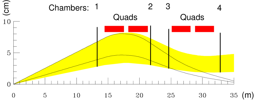
Figure 4: Particle trajectories through a UA8 Roman-pot spectrometer. The labels, “Quads”, refer to the low-$\beta$ machine quadrupole magnets. The center of the UA2 detector is at $z=0$ at the left of the sketch. The vertical lines indicate the positions of the UA8 wire chambers in the Roman-pots. The solid curves show the trajectories of 300 GeV particles ($\mbox{$x_{p}$}\sim 0.95$), as described in the text. The shaded area shows the allowed trajectories for $\mbox{$x_{p}$}=1$ tracks.

UA8 constructed Roman-pot spectrometers [12] in the same interaction region as UA2, in order to measure the outgoing “beam-like” $p$ and/or $\bar{p}$ in React. 1 or React. 2, together with the central system using the UA2 calorimeter system [13]. There were four Roman-pot spectrometers (above and below the beam pipe in each arm) which measured $p$ and/or $\bar{p}$ with $\mbox{$x_{p}$}>0.9$ and $0.8<|t|<2.5$ GeV². Fig. 4 shows one spectrometer with the trajectories of 300 GeV particles ($\mbox{$x_{p}$}\sim 0.95$) emerging from the center of the intersection region with minimum and maximum acceptable angles (solid curves). The lower (upper) edge of the shaded area corresponds to the minimum (maximum) accepted angles of $\mbox{$x_{p}$}=1$ tracks. The trajectory corresponding to the lower edge of the shaded region is 12 beam widths ($\sigma$) from the center of the circulating beam orbit.

Particle momenta in the Roman pot spectrometers were calculated in real–time by a dedicated special–purpose processor system [12, 27], thereby providing efficient low–rate $p$ and $\bar{p}$ triggers. Improved final-state proton and/or antiproton momenta are calculated offline using the reconstructed vertex position (if it exists), given by the UA2 central chamber system [13], and points reconstructed from hits in Roman pot chambers 1, 2 and 3. Chamber 4 was also used in the fit, if a track traversed it.

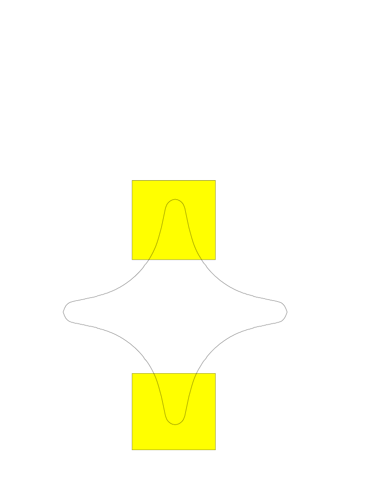
Figure 5: UA8 spectrometer aperture viewed from the interaction region. The shaded rectangles indicate the sensitive regions of the first wire chambers at a distance $z=13$ m from the interaction region center. The curved line indicates the walls of the beam pipe inside the quadrupole magnets.

Figure 5 shows a “beams-eye” view of the UA8 chamber aperture which is closest to the center of the interaction region. The four-lobed curve in the figure illustrates the contour of the beam pipe which matches that of the quadrupole-magnet pole pieces. The overlap between the beam pipe and rectangular chambers above and below the beam illustrates the limited azimuthal ranges in which a particle may be detected. These are centered at $\phi\sim 90^{\circ}$ and $\phi\sim 270^{\circ}$. Data were recorded with the bottom edge of each pot set, in different runs, at either 12 beam widths (12$\sigma$) or 14$\sigma$ from the beam axis.

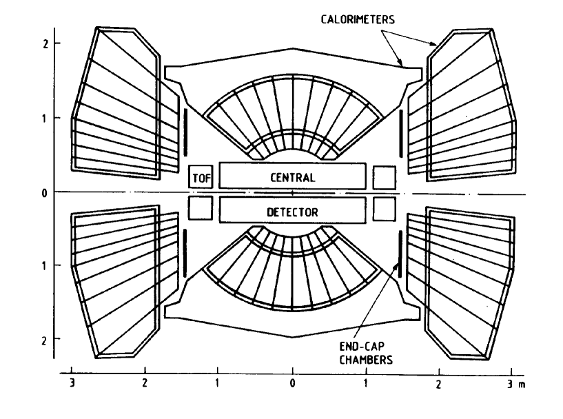
Figure 6: A cross sectional view of the upgraded UA2 apparatus. Detectors which were used for the measurements reported here are the Calorimeters, the Time–Of–Flight (TOF) counters and the Silicon Vertex Detector within the Central Detector assembly. The TOF counters covered pseudorapidity from 2.3 to 4.1 in each arm.

The upgraded UA2 calorimeter system [13], shown in Fig. 6, covered the polar angular range, $6^{\circ}<\theta<174^{\circ}$, and was used to measure the central system, $X$. In order to isolate React. 1 from other (background) events, rapidity–gaps are imposed offline between $p$ and $X$, and between $\bar{p}$ and $X$, by requiring the absence of charged–particle hits in the UA2 Time–Of–Flight (TOF) counters. These counters are indicated in Fig. 6 and cover the range of pseudorapidity, $2.3<|\eta|<4.1$, in both arms ($2^{\circ}$–$12^{\circ}$ and $168^{\circ}$–$178^{\circ}$). Since the TOF counters have some overlap with the small–angle region of the end–cap calorimeters, the calorimeter minimum acceptance angle for the events considered here is increased from $6^{\circ}$ to $12^{\circ}$ in both arms.

2.1 Triggering

Since the main goal of the UA8 experiment was to make measurements of hard-diffraction scattering in React. 2 [4, 5], UA8 was interfaced to the UA2 data acquisition system, which allowed the formation of triggers based on various combinations of $p$ and/or $\bar{p}$ momenta and transverse energy in the UA2 calorimeter system. Parallel triggers were also employed to yield samples of elastic and inelastic diffraction reactions with no conditions on the energy in the calorimeter system.

In order to find evidence for React. 1, one of the supplementary triggers required detection of a non-collinear $p$ and $\bar{p}$ pair. The $p$ and $\bar{p}$ were both required to be either in the “UP” spectrometers (above the beam pipe), as shown in Fig. 7(a), or in the “DOWN” spectrometers (below the beam pipe).

During the 1989 run, 1297 events were recorded in which both $p$ and $\bar{p}$ tracks were detected and the calorimeter system had a total recorded energy greater than 0.25 GeV. The remainder of the event-selection procedure for these events is described in Sect. 3.1.

The essential topology characteristic of these events is summarized in Table 1. It is seen that, when both $p$ and $\bar{p}$ have $\mbox{$x_{p}$}>0.95$, 48% of the events have rapidity–gaps in both arms (with pseudorapidity, $2.3<|\eta|<4.1$). However, when one or the other of the tracks has $\mbox{$x_{p}$}<0.95$, the percentage which possess rapidity–gaps in both arms falls to only a few percent. Thus, the first class of events appears to constitute a unique set, distinct from those events in which either $p$ or $\bar{p}$ have $\mbox{$x_{p}$}<0.95$.

A secondary data sample of React. 1 was extracted from data which were triggered by requiring that either $p$ or $\bar{p}$ is observed, as shown in Fig. 7(b). In these events, since there is no selection bias on momentum transfer, $t$, of the undetected particle, its natural distribution prevails, with an average value, $|t|\approx 0.2$ GeV². There were 62,627 such events recorded, after offline cuts for pile-up, beam-pipe geometry and halo cuts are made [2]. These data are dominated by single diffraction, React. 2. However, we show in Sect. 3.2 that the offline imposition of the rapidity–gap veto in both arms isolates React. 1 in this data sample.

3 Event selection

We henceforth refer to the event sample for which both $p$ and $\bar{p}$ were required in the trigger as the “AND” data sample. The events for which either $p$ or $\bar{p}$ are detected are referred to as the “OR” data sample.

3.1 “AND” data sample

The four constraints of energy-momentum conservation can be examined in individual events because the entire final state of React. 1 is seen in the Roman-pot spectrometers and the calorimeter system.

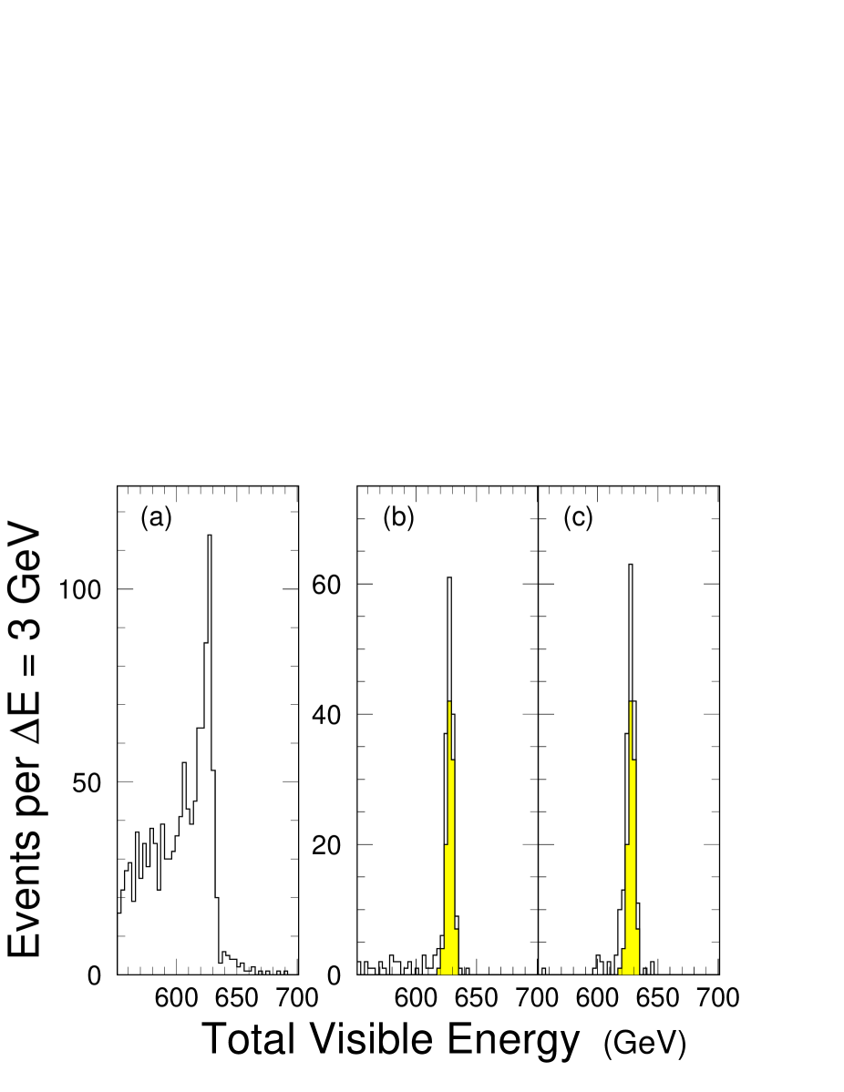
Figure 8: (a) Total visible energy in “AND” triggered events (1297) with total calorimeter energy, $\Sigma E>250$ MeV, selected offline; (b) Open histogram contains events (188) after veto using TOF counters, as discussed in the text. Shaded events (107) are after momentum conservation cuts (Figs. 9); (c) Open histogram are events (193) after momentum conservation cuts, but before TOF cuts. Shaded events are after the TOF cuts (107 events).

Fig. 8(a) shows the distribution of total visible energy ($p$ and $\bar{p}$ and central system, $X$) for these events. Although there is clearly a component of events which possess the full available energy of 630 GeV, a significant fraction of the events have less energy. Fig. 8(b) shows the same distribution, but for those events in which rapidity–gaps have been imposed using the Time–Of–Flight (TOF) counters in both arms. 188 events remain in a clean signal at 630 GeV.

Having seen that the energy constraint is well satisfied, we now consider the three momentum constraints. As implied by Fig. 7(a), a minimum accepted transverse momentum of $\sim 1$ GeV for each of $p$ and $\bar{p}$ corresponds to a net transverse momentum imbalance, $\mbox{${P_{t}}$}>2$ GeV, which is compensated for by a corresponding (opposite) momentum vector in the UA2 calorimeter system. In order to observe this, we define a summed momentum vector in the calorimeter. The cell energies observed in the UA2 calorimeter system are summed up as (massless) vectors to approximate the total momentum vector, $\vec{P}(X)$, of the system $X$ in React. 1. The azimuthal angle of $\vec{P}(X)$, $\Phi_{X}$, is plotted in Fig. 9(a) vs. the azimuthal angle of the summed momentum vector of the final-state $p$ and $\bar{p}$ particles. There are peaks seen at $90^{\circ}$ and $270^{\circ}$, corresponding to the cases where both $p$ and $\bar{p}$ are both in their DOWN spectrometers or both in their UP spectrometers (as sketched in Fig. 1(b)), respectively. Although $\Phi_{X}$ has no acceptance or trigger bias, in both cases it is seen to be opposite the azimuthal angle of the summed $p\bar{p}$ momentum vector in the figure.

The projection of the points in Fig. 9(a) on the $\Phi_{X}$ axis is shown in Fig. 9(b). The different intensities in the two peaks are due to small differences in the distances of the Roman-pots from the beam axis in the two spectrometers, resulting in a mismatch in their low–${P_{t}}$ cutoffs. The solid curve is a Monte–Carlo calculation and shows that the width of the peaks is understood. We select 139 events with $\Phi_{X}$ in the bands $90^{\circ}\,\pm\,20^{\circ}$ and $270^{\circ}\,\pm\,20^{\circ}$.

Although the summed transverse momentum of $p$ and $\bar{p}$, $\mbox{${P_{t}}$}(\mbox{$p$}+\mbox{$\bar{p}$})$, drops off sharply below 2 GeV, the transverse component of the calorimeter vector, $P_{t}(X)$, shown in Fig. 9(c) displays a much broader distribution due to the resolution of the calorimeter and the fact that, at small particle energies, some energy is lost before the particles reach the sensitive volume of the device. Fig. 10(a) shows the transverse projection of the calorimeter momentum vector together with the result of a Monte–Carlo simulation [28, 29] of the UA2 calorimeter system. This shows that the UA2 calorimeter simulation software does a good job in describing the calorimeter’s low energy response. We select 126 events with $1<\mbox{${P_{t}}$}(X)<3$ GeV for further analysis.

The degree of longitudinal momentum balance is demonstrated in Fig. 9(d), a histogram of total longitudinal momentum, $\Sigma P_{long}$, which includes the $p$, $\bar{p}$ and calorimeter longitudinal energies. A final sample of 107 DPE events satisfies the selection, $|\Sigma P_{long}|<7$ GeV. The shaded histogram in Fig. 8(b) shows the total visible energy for these events and demonstrates how well the energy constraint is satisfied. Fig. 8(c) is essentially the same as Fig. 8(b), except that the order of the TOF veto and momentum–conservation cuts is inverted.

Table 2 summarizes the event losses due to the cuts described here. They are compared with the effect of the same cuts on the Monte–Carlo generated events discussed in Sect. 4. The similarity between the two sets of numbers implies that most of the 188 events shown in Figs. 8(b) and 9(a,b) are in fact real examples of React 1.

An additional point can be made that there is an insignificant contribution in the data sample from events in which the observed proton comes from a diffractively–produced low–mass system (Baksay et al. [30] measured that this occurs ($12\pm 2.5$)% of the time). Such events would lead to an asymmetry and tail on the low side of the total visible energy distribution in Fig. 8. Although a small tail of this type does exist, it disappears when the momentum conservation cut is made. Thus we conclude that the rapidity–gap veto combined with momentum conservation eliminates this source of background.

3.2 “OR” data sample

As remarked above, the “OR” triggered sample is dominated by React. 2. However, the small component which is React. 1 can be isolated by selecting those events which possess rapidity–gaps in both arms.

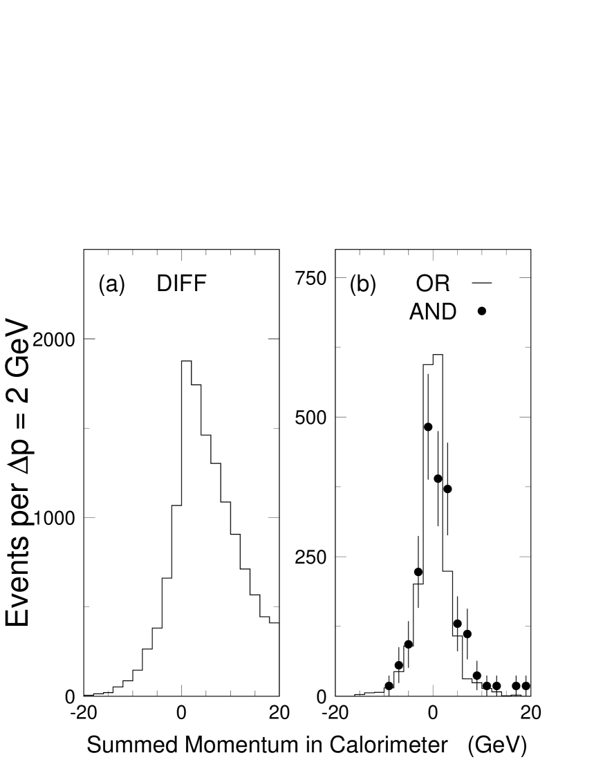
Figure 11: For “OR” triggered events, comparison of the summed longitudinal momentum in the calorimeter, with and without rapidity–gap veto (TOF). (a) Without TOF veto (the single–diffractive data sample); events are plotted on the positive axis if their summed momentum is in the hemisphere opposite the observed trigger particle. Events are required to have at least 250 MeV energy in the UA2 calorimeter system (partial sample, 15,080 events); (b) With rapidity–gap veto (1985 events). Solid points show the 107 “AND” events, normalized to the “OR” data.

A signature which distinguishes React. 1 from React. 2 is the presence of a longitudinally forward-backward symmetric distribution of particles in the UA2 calorimeter. Fig. 11(a) shows distribution of the summed longitudinal momentum component of all struck cells in the calorimeter for the triggered “OR” data sample. In constructing this plot, each event is plotted on the negative side if the summed vector is in the same hemisphere as the observed trigger particle, and on the positive side if the vector is in the opposite hemisphere. A large asymmetry is seen favoring the hemisphere opposite the trigger particle, as expected for React. 2.

Fig. 11(b) shows the subset of events in Fig. 11(a) which have no hits in any of the UA2 Time–Of–Flight counters. This corresponds to rapidity–gaps in the range $2.3<|\eta|<4.1$ in both arms. The forward-backward asymmetry seen in the calorimeter system disappears. The “AND” events are also plotted in Fig. 11(b) and are seen to have the same summed calorimeter momentum distribution as do the “OR” events. We take the events in the resulting symmetric distribution as the candidates for React. 1.

The next step in the selection of React. 1 is to look at the equivalent of Fig. 9(b) for this sample, namely the azimuthal angle, $\Phi_{X}$, of the summed calorimeter vector. Fig. 12(a) shows its distribution for those single-diffractive events in which the observed $p$ or $\bar{p}$ is seen in the DOWN spectrometer. Not surprisingly, a correlation is seen between the azimuthal angles of the observed $p$ or $\bar{p}$ and the summed calorimeter vector. However, when we make the “OR” event selection, by imposing the rapidity–gap condition using the TOF counters, we see in Fig. 12(b) that the correlation becomes much stronger. The distribution is broader than that seen in Fig. 9(b) for the “AND” events because of the unknown (small) ${P_{t}}$ of the unobserved final–state $p$ or $\bar{p}$ and also because of the smaller energy in the calorimeter. The Monte–Carlo simulation of the UA2 calorimeter is in reasonable agreement with the observed distribution. We select 698 “OR” events, with $\Phi_{X}$ either in the range $90^{\circ}\,\pm\,20^{\circ}$ or $270^{\circ}\,\pm\,20^{\circ}$.

Finally, for these “OR” candidates, we examine the summed transverse momentum in the calorimeter shown in Fig. 10(b). Because this vector is opposite only one observed vector of the $p$ or $\bar{p}$, its average value is less than that seen in Fig. 10(a) for the “AND” sample. However, it also is in reasonable agreement with the Monte–Carlo simulation of the UA2 calorimeter.

Figure 13 shows that the momentum transfer ($t$) distribution of the “OR” events is in good agreement with that of the full single-diffractive data sample. This is consistent with our basic assumption that the flux factor is common to Reacts. 2 and 1. The lower statistics “AND” data sample (not shown here) is also compatible with the single–diffractive data.

3.3 Feynman-$x_{p}$ distribution

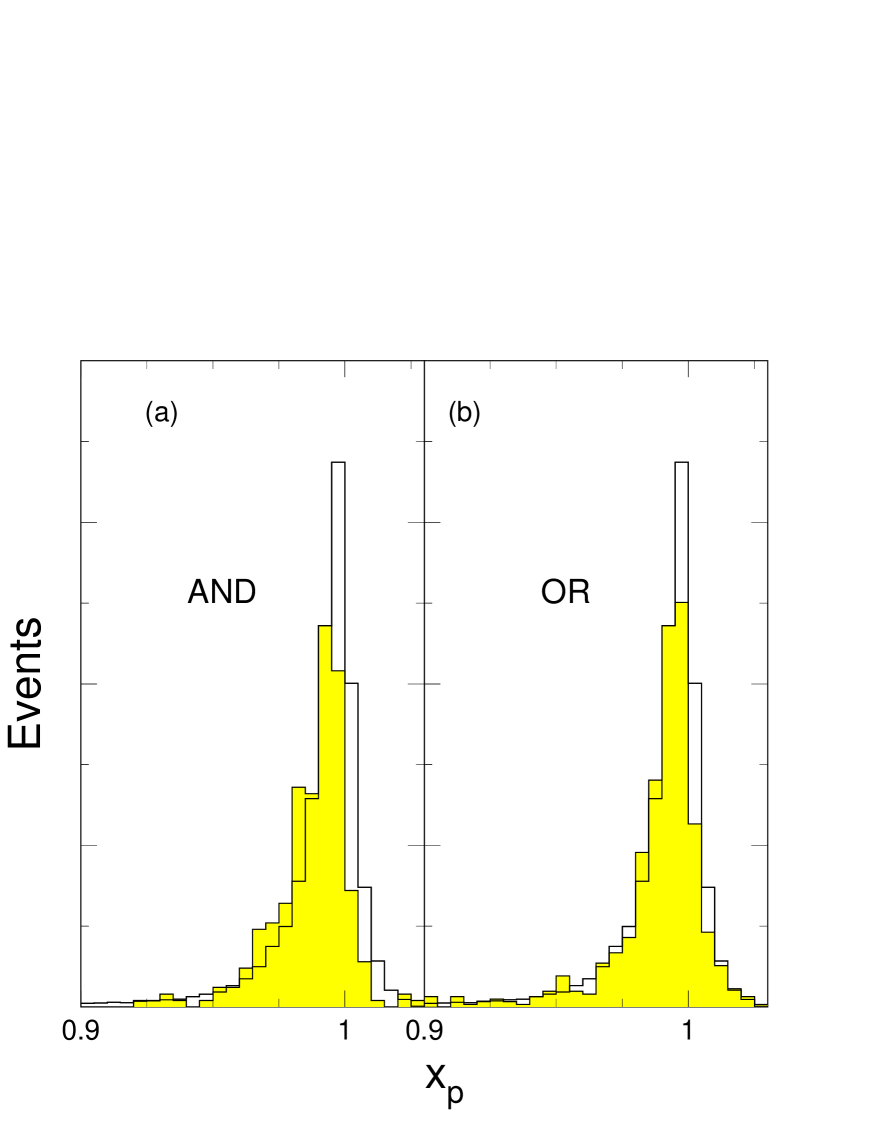
Figure 14: Feynman-$x_{p}$ distribution; (a) Shaded histogram is $x_{p}$ and $x_{\bar{p}}$ (2 points per event) for the “AND” events of React. 1 (139 events with TOF and $\Phi_{X}$ cuts). The open histogram is the $x_{p}$/$x_{\bar{p}}$ distribution from inclusive single diffraction [2], with a TOF veto only on the trigger side. The shaded and open histograms are normalized to the same area for the bin, $0.990<\mbox{$x_{p}$}<0.995$; (b) Same as (a), but the shaded histogram is $x_{p}$ or $x_{\bar{p}}$ for the “OR” data (698 events with TOF and $\Phi_{X}$ cuts). The vertical scale is linear.

The shaded distributions in Figs. 14(a,b) show the distributions of Feynman-$x_{p}$ and $x_{\bar{p}}$ for the final “AND” and “OR” data samples, respectively. They are essentially indistinguishable. The open histogram superimposed on both “AND” and “OR” distributions (shaded) in Fig. 14 is the $x_{p}$/$x_{\bar{p}}$ distribution in the single–diffractive data of React. 2 in our experiment [2]. In order that both sets of distributions have the same kinematic conditions, the single–diffractive data are plotted only for those events that have no hits in the TOF counters on the trigger side, which cover pseudorapidity, $2.3<\eta<4.1$. Each open histogram is normalized to its shaded distribution for the bin: $0.990<\mbox{$x_{p}$}<0.995$.

We see that the single–diffractive data possess a significant event population for $x_{p}>0.995$, which is not seen in either set of data for React. 1. As discussed in the Introduction and in Sect. 4, this apparent breakdown of factorization is merely a kinematic suppression in React. 1, due to the requirement that $s^{\prime}>0$ for the two–$\rm{\cal P}$omeron system. In the Monte–Carlo generation of two independently–emitted $\rm{\cal P}$omerons according to Eq. 5 (see Sect. 4), 61% of all events, in which both $p$ and $\bar{p}$ have $|t|>1$ GeV², have $s^{\prime}<0$ and are discarded. The rejected events mostly have small–$\xi$; for example, when either $\rm{\cal P}$omeron has $\xi<0.0005$, 100% of the events are rejected, whereas when $\xi\approx 0.03$, only 26% of the events are rejected. This qualitatively accounts for the difference between DPE and single diffractive data near $x_{p}$ = 1 in Fig. 14. For the “OR” topology, when only one $|t|>1$ GeV², the rejection at small–$\xi$ is about the same (95%), whereas there is more rejection at $\xi=0.03$ (51%); this accounts for the small difference in shape between “AND” and “OR” data in Fig. 14. The detailed shapes of these distributions depend on $\sigma_{{\cal P}{\cal P}}^{tot}$, which we have not yet determined.

4 Monte–Carlo event generation

A complete Monte–Carlo simulation [29] of React. 1 was performed to determine the spectrometer and calorimeter acceptances as well as the efficiencies of the various cuts. Events were generated such that the $\rm{\cal P}$omerons are emitted independently from proton and antiproton, respectively, according to Eq. 5, using the $\rm{\cal P}$omeron flux factor [19, 2] in Eq. 3. $\sigma_{{\cal P}{\cal P}}^{tot}$ is assumed to be independent of $s^{\prime}$, although in Sect. 6 we will look for departures from this assumption.

Points were chosen randomly in the 6-dimensional space, ($t_{1},\,\xi_{1},\,\phi_{1},\,t_{2},\,\xi_{2},\,\phi_{2}$), according to the product of two flux factors. Each such point defines the properties of the $\rm{\cal P}$omeron–$\rm{\cal P}$omeron system, its energy and its momentum vector. We have observed that, even though the two $\rm{\cal P}$omerons are assumed to be independently emitted, not all points in the 6–dimensional space are kinematically allowed because the associated $\rm{\cal P}$omeron-$\rm{\cal P}$omeron invariant mass may be unphysical (i.e., $s^{\prime}<0$). Thus, events are retained only if they are in regions of the 6-dimensional space for which $s^{\prime}>0$. In our $|t|$-domain, 1–2 GeV², such events are 39% of the total generated. We note that, even though the $\rm{\cal P}$omerons are generated isotropically and independently in azimuthal angle, $\phi$, correlations occur due to this kinematic suppression.

The number of particles of the central system, $X$, in React. 1 is generated according to a Poisson distribution with its mean charged particle multiplicity depending on $M_{X}$, as measured in a study of low-mass diffractive systems [31], $\bar{n}=0.6M_{X}$ ($M_{X}=\mbox{$\sqrt{s^{\prime}}$}$ in GeV); the mean number of neutral particles is assumed to be one-half the number of charged particles. The tracks are generated isotropically in the $M_{X}$ center-of-mass (see Sect. 5). As described in Sect. 5.2, where the central system is seen to have longitudinal structure for $M_{X}>5$ GeV, the Monte–Carlo generator is tuned to agree with the data.

After phase-space generation of the complete events, their data were passed through detector simulation software for both the UA8 spectrometers and the UA2 detectors [28], and then through the same offline analysis software and cuts used for the real data.

As already discussed in Sect. 3, Table 2 shows the good agreement between the real event losses with the momentum cuts described in Sect. 3 and those on the Monte–Carlo events calculated here. Since the Monte–Carlo event sample of React. 1 suffers a 46% loss when the TOF veto is imposed, the net efficiency for event retention due to TOF veto and event selection cuts is 26%.

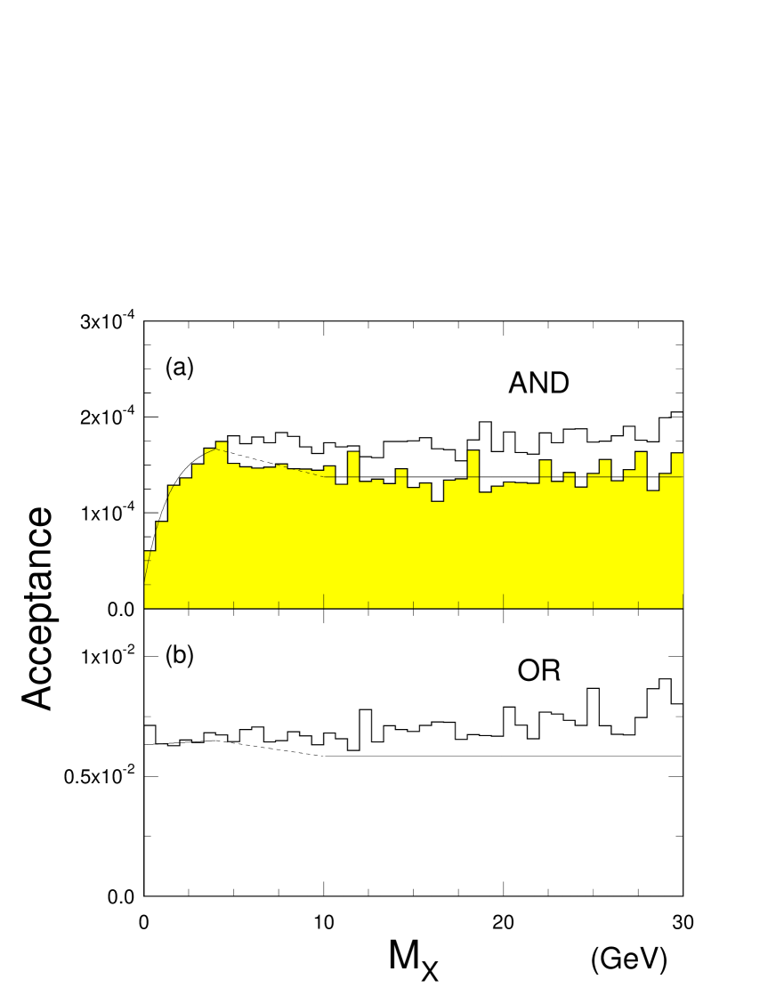
Figure 15: Geometrical acceptance and track reconstruction efficiency vs. $M_{X}$. As described in the text, retention efficiencies of TOF veto cut and event selection are included; (a) “AND” triggered events with $p$ and $\bar{p}$ both having $1.0<-t<2.0$ GeV². As discussed in the text, the open histogram assumes isotropic decay and the shaded histogram assumes longitudinal decay, for $M_{X}>4$ GeV. The combination of solid and dashed curves is the acceptance function used in cross section calculations; (b) “OR” triggered events with $1.0<-t<2.0$ GeV² for the observed final-state particle assuming isotropic decay. The solid line for $M_{X}>10$ GeV is the assumed acceptance for longitudinal decay which, as for the “AND” data, is $\approx 25\%$ smaller than the acceptance for events with isotropic decay.

The combined geometric and detection efficiency of proton and antiproton is about $6\cdot 10^{-4}$ at an average $|t|$ of 1.2 GeV². Figures 15(a,b) show the $M_{X}$–dependence of the overall geometric and detection efficiencies averaged over all other variables, for “AND” and “OR” data, respectively, when the observed particles are in the range, $1.0<-t<2.0$ GeV². The 26% central system detection efficiency is also included in these efficiencies. The fall–off in acceptance for the “AND” data at low mass results from the fact that, kinematically, low–mass events tend to have back–to–back $p$ and $\bar{p}$, which do not satisfy the “AND” trigger topology seen in Fig. 7. The “OR” trigger topology does not have such a bias against low–mass events.

The longitudinal structure seen in Sect. 5.2 for central system masses larger than about 5 GeV must impact the acceptance of the central system. Thus, we show the “AND” acceptances in Fig. 15(a), first assuming isotropic decay of the central system and then, for $M_{X}>4$ GeV, with a longitudinal decay distribution which matches that which is observed. At large mass, the acceptance for longitudinal decay is 25% smaller than the acceptance for isotropic decay. Since, with our statistics, it is not possible to properly study the transition from isotropic to longitudinal decay, we take the effect into account in the following way. For $M_{X}<4$ GeV, we use the calculated acceptance for isotropic decay, shown as the solid curve. For $M_{X}>10$ GeV, we use the fitted horizontal solid line in the figure. In the intermediate range, between 4 and 10 GeV, the dotted interpolation line is used.

For the “OR” acceptance at low mass ($M_{X}<4$ GeV), we use the calculated acceptance for isotropic decay in Fig. 15(b), just as we did for the “AND” data. For $M_{X}>10$ GeV, we use the solid horizontal line which is 25% below the calculated efficiency for isotropic decay. Again, the dashed interpolation line is used in the intermediate region.

5 Calorimeter measurement of central system

We use the UA2 calorimeter information to study the invariant mass and other properties of the central system, $X$, in React. 1. The UA2 detector simulation software [28] was used to perform a complete Monte–Carlo study of the calorimeter response. As noted above, the UA2 simulation software is remarkably good in describing the low-energy deposits encountered in our data.

5.1 Invariant mass of central system

Since we do not directly observe the individual particles of this system, but rather the energies deposited in the calorimeter cells, we assume that the non-zero energy in each “struck” cell of the calorimeter is caused by a massless particle, and then calculate,

$${M_{observed}}^{2}=(\Sigma E_{i})^{2}-|\Sigma\vec{P}_{i}|^{2},$$ (7)

summing over all cells.

Figure 16 is the result of a Monte–Carlo study [29] which shows that this procedure underestimates the true mass by an amount that increases with mass. This effect results from incomplete detection of energy; for example, the finite cell size leads to overlapping energy deposits from neighboring particles, or some energy can be lost before the particles enter the calorimeter. The difference between the true MC mass, $M_{true}$, and the calculated or observed mass, $M_{observed}$, is plotted vs. $M_{true}$. The dependence is well fit by the equation (with $M$ in units of GeV): $M_{true}-M_{observed}=(1+4M_{true})/14$, which can be rewritten as:

$$M_{true}\,\,=1.4\,M_{observed}\,\,+\,\,0.1.$$ (8)

We define the corrected mass, $M_{X}^{2}=s^{\prime}$, to be the true mass given by this equation and only refer to these corrected values in the remainder of this paper.

The validity of the calorimeter invariant mass calculation may be conveniently tested by comparing it with the missing mass calculated using the measured $p$ and $\bar{p}$ 4-vectors for an event. Although the experimental uncertainty in a “missing mass” calculation is much larger than for the calorimeter invariant mass, they should agree on average. Fig. 17 shows the average missing mass calculated for the events in each of the calorimeter invariant mass bins shown in the figure. The observed clustering of the points around the diagonal and the absence of any systematic shifts constitutes proof that the calorimeter mass evaluation is reliable.

The $M_{X}$ distributions of the system $X$ in React. 1 are shown for the final selected “AND” and “OR” event samples in Figs. 18(a,b), after requiring that the momentum transfer of all detected protons and antiprotons be in the range, 1–2 GeV². From the relatively flat acceptance curves in Figs. 15(a,b), we see that the observed shapes of the distributions are reasonably good representations of the true distributions (except for the lowest mass bin in the “AND” data) . In Sect. 6.1, we show that part of the low–mass enhancements are attributable to an explicit $s^{\prime}$ dependence in $\sigma_{{\cal P}{\cal P}}^{tot}$, corresponding to an enhanced $\rm{\cal P}$omeron–$\rm{\cal P}$omeron interaction in the few-GeV mass region. However, with an estimated 1.8 GeV mass resolution obtainable from the calorimeter, we are unable to observe details of any possible $s$-channel resonant structure in this spectrum.

5.2 Other properties of the central system

In addition to the invariant mass distribution of the system, $X$, other properties of the system can be studied. One is the particle multiplicity of the central system. Figure 19 shows the number of calorimeter cells struck as a function of the corrected calorimeter mass, $M_{X}$. The solid line is a fit to the data; the dashed line is based on the naive multiplicity expectation assuming [31] $<N>=0.6M_{X}$ ($M_{X}$ in GeV) for the number of charged particles ($\pi^{+}$ and $\pi^{-}$). The number of $\pi^{0}$ is assumed to be Poisson–distributed with a mean of 0.3$M_{X}$; each of these is assumed to appear as two $\gamma$. The resulting dashed line is the function $N=1.2M_{X}$ and clearly captures the gross features of the data. The observed numbers of struck cells lie somewhat above the line, as expected geometrically from the cluster widths in the calorimeter and the finite cell sizes. A complete Monte–Carlo simulation [29] accounts for the small observed differences. We can conclude that the number of observed struck cells increases with mass roughly as expected, and the total observed multiplicity displays no anomalous features.

Because of the separated electromagnetic and hadronic section of the UA2 calorimeter, it has also been possible to study the fraction of electromagnetic energy possessed by the central system. Fig. 20 shows the distribution in this fraction for the “AND” events in the low-mass enhancement, $M_{X}<6$ GeV, compared with the Monte–Carlo generated distribution assuming, on the average, equal numbers of $\pi^{+}$, $\pi^{-}$ and $\pi^{0}$ in the track generation. Again we see no anomalous features in this variable. The enhancement visible in both data and Monte–Carlo when the ratio, (e.m. energy)/(total energy), equals unity corresponds to low mass systems where the slow pions deposit all their energy in the electromagnetic calorimeter cells.

We have examined the angular distributions of calorimeter cell energies in the center-of-mass of the $X$ system, $dN/dcos\theta$, with respect to the $\rm{\cal P}$omeron-$\rm{\cal P}$omeron direction of motion. Figs. 21(a,b) show these distributions for $M_{X}<5$ GeV and $M_{X}>5$ GeV. At the higher masses we see a similar type of forward–backward peaking as is seen in all hadronic interactions as a result of the presence of spectator partons. In the present case, this would imply that there are spectator partons in the $\rm{\cal P}$omeron. We have already reported [2, 32] similar effects in $\rm{\cal P}$omeron-proton interactions in the single-diffractive, React. 2.

The Monte–Carlo histogram in Fig. 21(a) shows isotropically-decaying events. In Fig. 21(b), the histogram shows a Monte Carlo event sample which has been selected in such a way that it has the same forward–backward peaking as the experimental distribution. For each isotropically–decaying Monte–Carlo event, the mean value of $cos^{2}\theta$ is evaluated averaging over all outgoing tracks in the central system. We have found [29] that, if Monte–Carlo events are selected for which this quantity is larger than 0.375, the selected events follow the experimental $cos\theta$ distribution.

6 Cross sections

The observed mass distributions, $dN/dM_{X}$, shown in Figs. 18(a,b) for the “AND” and “OR” data, respectively, are converted into absolute cross section distributions, $d\sigma_{DPE}/dM_{X}$, in the following way. Bin–by–bin, the numbers of events in Figs. 18 are divided by the Monte–Carlo acceptance curves in Figs. 15(a,b). Then, all are divided by a global efficiency, $\epsilon_{0}$, for event retention when halo and pileup cuts [12, 29] are made, and by the appropriate integrated luminosity for each trigger sample:

$$\Delta\sigma_{DPE}\,\,=\,\,{{\Delta N}\over{\int{\cal L}dt\cdot\epsilon_{0}\cdot A}}.$$ (9)

The “AND” (“OR”) data samples have an efficiency, $\epsilon_{0}$, of 0.54 (0.76) and an integrated luminosity, $\int{\cal L}dt$, of 2894 nb^-1 (5.4 nb^-1). The “OR” luminosity is “effective”, due to prescaling of the “OR” trigger. In both cases, the cross section is given only for momentum transfer of the observed trigger particle(s) in the range: $1.0<|t|<2.0$ GeV². In the “OR” case, the unseen $p$ or $\bar{p}$ has its “natural” ${P_{t}}$ distribution and therefore peaks at small values. Thus, the observed cross section is much larger for the “OR” data. The resulting cross sections for the two triggered data samples of Reaction 1, $d\sigma/dM_{X}$, are the points shown in Figs. 22(a,b).

6.1 $\rm{\cal P}$omeron–$\rm{\cal P}$omeron total cross section

We now extract the $\rm{\cal P}$omeron–$\rm{\cal P}$omeron total cross section, $\sigma_{{\cal P}{\cal P}}^{tot}$, from the data, so that we can look for deviations from our earlier assumption that it is independent of $M_{X}$. The histograms in Figs. 22(a,b) are Monte–Carlo predictions for the $d\sigma_{DPE}/dM_{X}$ points in the figure, made using Eq. 5 and $F_{{\cal P}/p}(t,\xi)$ in Eq. 3. We assume a constant $\rm{\cal P}$omeron–$\rm{\cal P}$omeron total cross section of $\sigma_{{\cal P}{\cal P}}^{tot}$ = 1 mb and the (arbitrary) value, $K=0.74$ GeV^-2, as discussed in Sect. 1.

Since the UA8 spectrometer acceptances [2] do not vary significantly over the range of $\xi$ studied here, the ratios of the points to the histogram values in Figs. 22 give values of the $\rm{\cal P}$omeron-$\rm{\cal P}$omeron total cross section, $\sigma_{{\cal P}{\cal P}}^{tot}$, vs. $M_{X}$. These ratios are shown in Fig. 23, for both the “AND” and “OR” data. We note that, despite the large difference between the measured cross sections, $d\sigma_{DPE}/dM_{X}$, in Figs. 22(a,b), both data sets yield the same general properties for $\sigma_{{\cal P}{\cal P}}^{tot}$: enhancements for $M_{X}<8$ GeV and relatively $M_{X}$ independent shapes at larger $M_{X}$. Although the two values of $\sigma_{{\cal P}{\cal P}}^{tot}$ in the first bin ($M_{X}<2$ GeV) are consistent with being equal, in the next three bins ($2<M_{X}<8$ GeV) the “AND” cross sections are about three times larger than the “OR” cross sections. However, only the statistical errors on $\sigma_{{\cal P}{\cal P}}^{tot}$ are shown in Fig. 23. We discuss their systematic uncertainties in the following section.

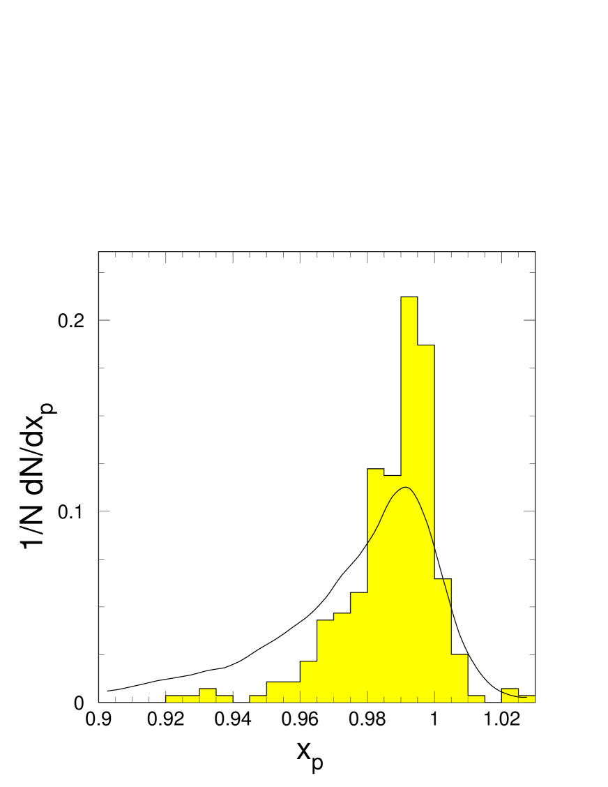
Figure 24: $x_{p}$ ($x_{\bar{p}}$) distribution for the “AND” data as in Fig. 14(a). The solid curve normalized to the data is the Monte–Carlo prediction assuming no explicit $s^{\prime}$–dependence in $\sigma_{{\cal P}{\cal P}}^{tot}$.

The small–$M_{X}$ enhancement in Fig. 23 also reflects itself in the observed $x_{p}$ ($x_{\bar{p}}$) distributions seen above in Figs. 14. Such a correlation must exist because of the kinematic relation, ${M_{X}}^{2}=s^{\prime}=\xi_{1}\xi_{2}s$; small $M_{X}$ correlates with small $\xi$. Fig. 24 repeats the $x_{p}$ ($x_{\bar{p}}$) distribution for the “AND” data in Fig. 14(a). The solid curve normalized to its area is the Monte–Carlo prediction which assumes an $s^{\prime}$–independent $\sigma_{{\cal P}{\cal P}}^{tot}$. The pronounced excess of events near $x_{p}$ = 1.0 in the experimental distribution, compared with the Monte–Carlo distribution, is another manifestation of the low–mass enhancement in $\sigma_{{\cal P}{\cal P}}^{tot}$.

The low–mass enhancements seen in both distributions in Figs. 23 are most likely too large[33] to be due to a breakdown of factorization at small mass, especially for the “AND” data. Thus, the rise may indicate that glueball production is a significant component of the low-mass $\rm{\cal P}$omeron-$\rm{\cal P}$omeron interaction, although not necessarily an $s$-channel effect. That is, the observed invariant mass could be that of a glueball $\it plus$ other particles, which would not lead to resonance structure in the mass distribution. In any case, with a mass resolution of $\approx 1.8$ GeV, no $s$–channel structure could be seen.

6.2 Systematic uncertainties

We now ask how possible systematic uncertainties influence the interpretation of the $\sigma_{{\cal P}{\cal P}}^{tot}$ results shown in Fig. 23. A systematic uncertainty common to both sets of cross section results comes from the Monte–Carlo acceptance shown in Fig. 15. We estimate that this uncertainty is smaller than 15%. In the case of the “AND” results, the statistical errors are much larger than this.

There is an additional systematic uncertainty that is very different for the “AND” and “OR” results. This arises from the possible non-universality of the $\rm{\cal P}$omeron flux factor. It is already known that $F_{{\cal P}/p}(t,\xi)$ is not universal between $ep$ and $p\mbox{$\bar{p}$}$ collisions because of the different effective $\rm{\cal P}$omeron trajectory intercepts found in the two cases, attributable to different multi–$\rm{\cal P}$omeron–exchange effects. Similarly, if multi-$\rm{\cal P}$omeron-exchange is not identical in Reacts. 1 and 2, there would be some uncertainty as to whether the same flux factor should appear in both Eqs. 5 and 3.

We note, however, that this potential uncertainty does not exist for the “AND” results, because both final–state baryons have $|t|>1.0$ GeV², where all the evidence[17, 19] points to an $s$–independent $\rm{\cal P}$omeron trajectory; in that high–$|t|$ region, $F_{{\cal P}/p}(t,\xi)$ appears to be insensitive to the damping which mainly leads to an $s$–dependent effective $\rm{\cal P}$omeron intercept[19] at $t=0$. Thus, the statistical errors on the “AND” results in Fig. 23 dominate any uncertainties from this source.

The situation is very different for the “OR” data sample because the unseen final–state baryon has low–$|t|$ and its flux factor in Eq. 5 is sensitive to the choice of effective $\epsilon$ value. We have thus recalculated the “OR” cross sections in Fig. 23 assuming a larger $\rm{\cal P}$omeron trajectory intercept, $\epsilon=0.10$, in $F_{{\cal P}/p}(t,\xi)$. This is an extreme (unrealistic) case which assumes that there are no damping contributions from multi–$\rm{\cal P}$omeron–exchange in React. 1 at our energy. We find that the “OR” cross sections decrease from those shown in the figure; for example, the lowest mass point decreases by 58%, whereas the point at 11 GeV decreases by 41%. Thus, any increase in the effective $\epsilon$ used in calculating $\sigma_{{\cal P}{\cal P}}^{tot}$ from the “OR” data increases the disagreement already observed in Fig. 23.

The final systematic uncertainty comes from our model assumption that there are no azimuthal angle correlations between final–state $p$ and $\bar{p}$ in Eq. 5, other than the kinematic one referred to in Sect. 1. However, the following two facts lead us to suspect that this may not be true: (a) there are differences between the “AND” and “OR” $\sigma_{{\cal P}{\cal P}}^{tot}$ results, and (b) the “AND” and “OR” data samples have very different $\rm{\cal P}$omeron–$\rm{\cal P}$omeron configurations. The difference in $\rm{\cal P}$omeron–$\rm{\cal P}$omeron configurations is most easily visualized with reference to our Fig. 7. In the upper figure (“AND”), it is seen that both $\rm{\cal P}$omeron transverse momenta, ${P_{t}}$, are approximately in the same direction; hence $\Delta\mbox{${P_{t}}$}\approx 0$. In the lower figure (“OR”), one transverse momentum is near zero and the other is near 1 GeV; hence the “OR” data sample corresponds to $\Delta\mbox{${P_{t}}$}\approx 1.0$ GeV.

Thus, the observed differences in $\sigma_{{\cal P}{\cal P}}^{tot}$ for the “AND” and “OR” data in Fig. 23 at low mass suggest that $\sigma_{{\cal P}{\cal P}}^{tot}$ depends on the $\rm{\cal P}$omeron–$\rm{\cal P}$omeron relative configuration and is larger at low mass when the two $\rm{\cal P}$omerons move approximately in the same direction. We also note that the systematic uncertainty due to our limited understanding of multi–$\rm{\cal P}$omeron–exchange effects can not be responsible for the effect now being discused, since it can only make the difference larger. We return to the physics of the present discussion in the concluding Sect. 7.

6.3 Test of factorization

We now test the factorization relation, Eq. 6, between $\sigma_{{\cal P}{\cal P}}^{tot}$, $\sigma_{{\cal P}p}^{tot}$ and $\sigma_{pp}^{tot}$. If we multiply both sides of Eq. 6 by $K^{2}$, we find:

$$K^{2}\cdot\mbox{$\sigma_{{\cal P}{\cal P}}^{tot}$}(s^{\prime})\,\,\,\,=\,\,\,\,{{[K\cdot\mbox{$\sigma_{{\cal P}p}^{tot}$}(s^{\prime})]^{2}}\over{\sigma_{pp}^{total}(s^{\prime})}}.$$ (10)

which relates precisely the measured quantities. Thus, it is evident that tests of factorization using Eq. 6 or 10 are equivalent and we may, with no loss of precision, assume the value, $K=0.74$ GeV^-2 (see discussion in Sect. 1), and make the test using Eq. 6.

In order to calculate the right-hand-side of Eq. 6 a function of $s^{\prime}$, we use the following parametrizations for the $\rm{\cal P}$omeron–proton total cross section [2]:

$$\mbox{$\sigma_{{\cal P}p}^{tot}$}={{0.72}\over{0.74}}\cdot[(s^{\prime})^{0.10}+4.0(s^{\prime})^{-0.32}]\,\,\,\,\,{\rm mb},$$ (11)

and for the proton-proton total cross section [34, 35]:

$$\mbox{$\sigma_{pp}^{tot}$}=18\cdot s^{0.10}-27\cdot s^{-0.50}+55\cdot s^{-0.32}\,\,\,\,\,{\rm mb}.$$ (12)

These functions are shown as the dashed curves in Figs. 25(a,b). Since Eq. 6 is only valid for the $\rm{\cal P}$omeron–exchange component of these functions, we show only the first terms in Eqs. 11 and 12 as the solid curves in the figures.

The dashed line in Fig. 23 shows the factorization prediction for $\sigma_{{\cal P}{\cal P}}^{tot}$ calculated using Eq. 6 and the $\rm{\cal P}$omeron terms in Eqs. 11 and 12:

$$\mbox{$\sigma_{{\cal P}{\cal P}}^{tot}$}(s^{\prime})\,\,\,\,=\,\,\,\,{{[\mbox{$\sigma_{{\cal P}p}^{tot}$}]^{2}}\over{\sigma_{pp}^{total}}}={{(0.72/0.74)^{2}}\over{18}}\cdot(s^{\prime})^{0.10}.$$ (13)

We see that there is increasingly better agreement between the prediction and the measured $\sigma_{{\cal P}{\cal P}}^{tot}$ points as the mass increases, as expected, since the measured points contain both $\rm{\cal P}$omeron exchange and $\rm{\cal R}$eggeon exchange. The results are seen to be in reasonable agreement with the validity of factorization for $\rm{\cal P}$omeron-exchange in these reactions.

The solid curve in Fig. 23 is a fit to the “OR” points with $M_{X}>10$ GeV of the sum of Eq. 13 and a $\rm{\cal R}$eggeon–exchange component as in Eq. 11:

$$\mbox{$\sigma_{{\cal P}{\cal P}}^{tot}$}(s^{\prime})\,\,\,\,=\,\,\,\,{{(0.72/0.74)^{2}}\over{18}}\cdot[(s^{\prime})^{0.10}+R\cdot(s^{\prime})^{-0.32}].$$ (14)

We find a value, $R=13.6\pm 4.7$, with a $\chi^{2}/{\rm D.F.}=1.3$.

7 Conclusions and predictions

Table 1 demonstrates that there is a new class of events, the so–called double–$\rm{\cal P}$omeron–exchange (DPE) events with characteristic rapidity–gaps in both arms, which appear when both $x_{p}$ values are greater than 0.95. The analysis which follows this observation shows that, remarkably, the Regge formalism describes all inclusive DPE and single–diffractive data, using the empirical $s$-dependent effective $\rm{\cal P}$omeron trajectory of Ref. [19], which is believed to be due to increasing multi-$\rm{\cal P}$omeron–exchange effects with energy [18]. That Regge phenomenology works as well as it does, despite the complications of multi-$\rm{\cal P}$omeron-exchange, should place constraints on a theory of such multi-$\rm{\cal P}$omeron–exchange effects yet to be developed.

We observe that the produced central systems in the DPE events display no anomalous multiplicity distributions or electromagnetic energy fraction of the total observed calorimeter energy. Our measurements agree with normal expectations.

The main result of the work reported here is the $\rm{\cal P}$omeron–$\rm{\cal P}$omeron total cross section, $\sigma_{{\cal P}{\cal P}}^{tot}$, shown in Fig. 23. At large mass, there is a statistically weak agreement with factorization predictions. However, for $M_{X}<8$ GeV, both the “AND” and “OR” results exhibit large enhancements in $\sigma_{{\cal P}{\cal P}}^{tot}$, with the “AND” result being about three-times larger than the “OR” result. There may be a dynamical reason for this, based on the fact that the “AND” and “OR” data sets have different $\rm{\cal P}$omeron–$\rm{\cal P}$omeron configurations.

These results are probably related to the WA102 Collaboration observations [36], at the much lower center–of–mass energy, $\sqrt{s}=29$ GeV, that the production of known quark-antiquark states and glueball candidates depend differently on the difference in transverse momenta of the two $\rm{\cal P}$omerons in React. 1. The primary WA102 effect is that the production of $q\bar{q}$ states appears to vanish as $\Delta\mbox{${P_{t}}$}\rightarrow 0.$ Close and Kirk [37] suggested that this effect may serve as a “glueball filter”. On the basis of the WA102 results, Close and Schuler [38] argue that the effective spin of the $\rm{\cal P}$omeron can not be zero and that the $\rm{\cal P}$omeron transforms as a non-conserved vector current.

Taken at face value, the WA102 results [36] imply that our “AND” data do not contain any $q\bar{q}$ states and, hence, that the enhancement for $2<M_{X}<8$ GeV in those data may be due to production of some glueball–like objects. There would be a mix of $s$-channel production (i.e. glueball alone) and production with other particles. The observation of resonant mass structure is precluded in the present experiment because of our poor mass resolution of $\approx 1.8$ GeV.

The next generation experiment of the type reported here should utilize a central detector capable of detailed studies of the produced central systems (including particle identification). In order to be able to observe the azimuthal angle correlations of the outgoing protons with properties of the central systems, the Roman–pot systems (on both arms) should have as full an azimuthal coverage as possible.

7.1 Predictions for Tevatron and LHC colliders

The fact that the “AND” and “OR” data yield essentially the same $\sigma_{{\cal P}{\cal P}}^{tot}$ at larger mass implies that our rapidity–gap procedures for isolating React. 1 are fundamentally sound and can used at the much higher energy experiments at the Tevatron and LHC to look for rare states with greatest sensitivity.

The study of the relatively pure gluonic collisions in React. 1 at higher energy colliders may yield surprising new physics. In the UA8 papers on the occurrence and study of jet events in single–diffraction [5], it was reported that, in about 30% of the 2-jet events, the $\rm{\cal P}$omeron appeared to interact as a single hard gluon with the full momentum of the $\rm{\cal P}$omeron (the so–called “Super–Hard” $\rm{\cal P}$omeron) . This result suggests that, in roughly 10% of hard $\rm{\cal P}$omeron–$\rm{\cal P}$omeron interactions, there is effectively a gluon-gluon collision with the full $M_{X}$ of the central system. Thus, for example, at the LHC with $\mbox{$\sqrt{s}$}=14$ TeV, a rather pure sample of central gluon-gluon collisions should occur with $M_{X}$ as large as 0.03(14) = 0.42 TeV (remember from Sect. 1 that we believe there is essentially pure $\rm{\cal P}$omeron exchange at $\xi=0.03$).

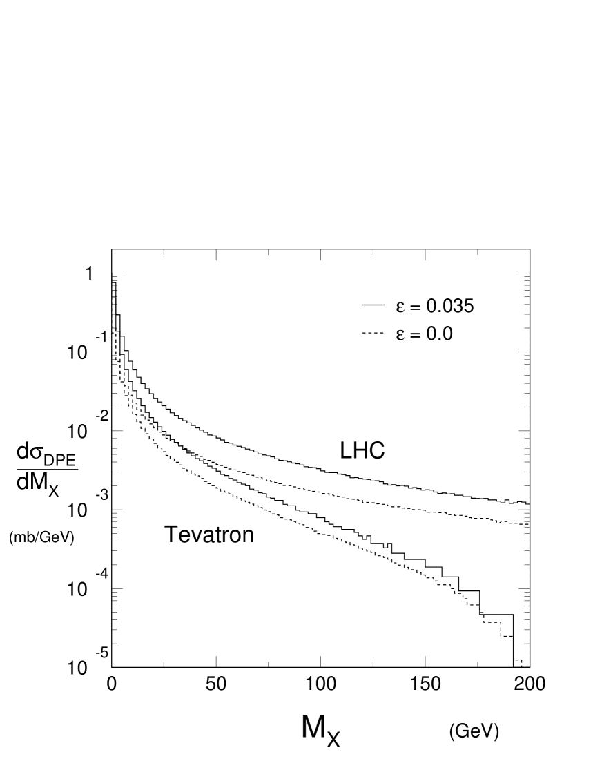
Figure 26: Predicted differential cross section $d\sigma_{DPE}/dM_{X}$ (integrated over all $t$), assuming constant $\sigma_{{\cal P}{\cal P}}^{tot}$ = 1 mb for the Tevatron ($\mbox{$\sqrt{s}$}=2$ TeV) and the LHC ($\mbox{$\sqrt{s}$}=14$ TeV). In each case, the solid (dashed) curves are for assumed effective $\rm{\cal P}$omeron intercepts, $\alpha(0)=1.035$ (1.00) respectively.

The phenomenology developed in our study of React. 1 can be used to make cross section predictions at the Tevatron ($\mbox{$\sqrt{s}$}=2$ TeV) and at the LHC ($\mbox{$\sqrt{s}$}=14$ TeV). Figure 26 and Table 3 show the results of Monte–Carlo calculations of $d\sigma_{DPE}/dM_{X}$ (integrated over all $t$), assuming that $\sigma_{{\cal P}{\cal P}}^{tot}$ is $M_{X}$–independent and constant at 1 mb. Since the fitted value [19] of the effective $\rm{\cal P}$omeron–Regge–trajectory intercept, $1+\epsilon$ = 1.035, at $\sqrt{s}$ = 630 GeV, is also compatible with the available data at the Tevatron, we give the results for $\epsilon=0.035$ at both Tevatron and LHC. Schuler and Sjöstrand [39] suggest, in a model of hadronic diffractive cross sections at the highest energies, that $\epsilon=0$ is a reasonable approximation and we therefore also give results for this value. The observed peaking at small mass directly reflects the $\xi$-dependence of the $\rm{\cal P}$omeron flux factor in the proton.

To obtain cross section predictions for central Higgs production [40] in React. 1 from the “Super–Hard” component of the $\rm{\cal P}$omerons , the calculations in Fig. 26 can be multiplied by the calculated QCD cross section for the process (in units of mb) based on the best available $\rm{\cal P}$omeron structure function.

We note that the cross section predictions obtained in this way give the total cross section for React. 1, where there are no selection cuts on either final–state $p$ or $\bar{p}$. Clearly this yields the largest sensitivity for rare events. In that case, if rapidity–gap vetos are used to suppress background events, corrections must be made for the acceptance loss of central system particles in the rapidity–gap regions.

7.2 Predictions for forward spectrometers

For completeness, it may be useful to briefly summarize the possibilities for detection of DPE processes using existing or planned forward multiparticle spectrometers. There are two classes of such experiments, those traditionally called fixed–target experiments and those installed at storage-ring colliders[41].

Forward spectrometers installed at colliders can observe DPE processes if there is an asymmetry between $\xi_{1}$ and $\xi_{2}$. The earliest example of such a measurement was Experiment R608 studying $pp$ interactions with $\sqrt{s}=63$ GeV at the Cern Intersecting-Storage-Rings. Central production of $D(1285)$ was observed[42] with almost pure helicity $\pm 1$, later explained by Close and Schuler [38] as due to the $\rm{\cal P}$omeron behaving as a non-conserved vector current. In that process, the $\rm{\cal P}$omeron appeared to dominate even though $\xi_{1}-\xi_{2}\approx 0.35$. In the future, the higher energy forward–spectrometer B–experiments, LHCb and B-TeV, will have good access to low-mass central systems with much smaller values of $\xi$, as was pointed out in the LHCb Letter–of–Intent[43].

In fixed-target experiments, centrally–produced systems are boosted forward with the $\gamma$ of the center–of–mass, such that $E_{Lab}=\gamma M_{X}$. Experiment WA102 [36] was the first experiment to carry out major DPE studies using this approach although, as commented above, with a beam energy of 450 GeV, the $\rm{\cal P}$omeron $\xi$–values were larger than desired. We note that the existing experiment, HERA-B[44], running at the HERA 920 GeV proton storage ring using wire targets, could improve on the WA102 measurements. For example, with $\sqrt{s}=42$ GeV, production of a 2-GeV central system occurs with an average $\xi=0.047$. Fig. 27 shows $d\sigma_{DPE}/dM_{X}$ for $pp$ interactions with a beam energy of 920 GeV, calculated as for Fig. 26. As indicated after Eq. 4, the $\rm{\cal P}$omeron trajectory intercept[19] used at this c.m. energy is: $1+\epsilon=1.087$.

$p$ or $\bar{p}$ has $\mbox{$x_{p}$}>0.95$	Number	Fraction with
Other has $x_{p}$ in bin	Events	rapidity–gaps
0.70-0.75	42	$0.02\pm 0.02$
0.75-0.80	113	$0.04\pm 0.02$
0.80-0.85	147	$0.07\pm 0.02$
0.85-0.90	163	$0.03\pm 0.02$
0.90-0.95	219	$0.06\pm 0.02$
0.95-1.00	314	$0.48\pm 0.04$

Table 1: Numbers of events and their fractions which have rapidity–gaps, $2.3<\eta<4.1$ in both arms, for different $x_{p}$ selections of $p$ and $\bar{p}$. 1297 events have two reconstructed tracks and at least 250 MeV of energy in the calorimeter system. The table shows the 998 events, in which either $p$ or $\bar{p}$ has $\mbox{$x_{p}$}>0.95$, while the other has $x_{p}$ in the indicated bin. In the remaining 299 events, for which both $p$ and $\bar{p}$ have $0.70<\mbox{$x_{p}$}<0.95$, only 0.7% possess both rapidity–gaps.

After	Events	percentage	MC percentage
Cut	remaining	remaining	remaining
TOF veto	188	–	–
$\Phi_{X}$	139	$74\pm 6$ %	72 %
${P_{t}}$	126	$67\pm 6$ %	60 %
$\Sigma P_{long}$	107	$57\pm 5$ %	50 %

Table 2: Comparison of event losses for data and Monte–Carlo events (after TOF veto) as a function of the 3-momentum cuts in the event selection.

$M_{X}$	$d\sigma_{DPE}/dM_{X}$ (mb/GeV)
	Tevatron		LHC
(GeV)	$\epsilon=0.00$	$\epsilon=0.035$	$\epsilon=0.00$	$\epsilon=0.035$
1	1.25E-01	2.69E-01	2.07E-01	7.55E-01
3	5.44E-02	1.00E-01	9.42E-02	2.96E-01
5	3.01E-02	5.17E-02	5.39E-02	1.58E-01
10	1.31E-02	2.11E-02	2.53E-02	6.76E-02
20	5.33E-03	7.65E-03	1.15E-02	2.75E-02
30	3.02E-03	4.14E-03	7.17E-03	1.62E-02
40	1.96E-03	2.57E-03	5.08E-03	1.13E-02
50	1.40E-03	1.78E-03	3.86E-03	8.34E-03
60	1.01E-03	1.25E-03	3.11E-03	6.45E-03
70	7.76E-04	9.42E-04	2.56E-03	5.23E-03
80	6.08E-04	7.15E-04	2.17E-03	4.32E-03
90	4.78E-04	5.54E-04	1.85E-03	3.75E-03
100	3.72E-04	4.21E-04	1.64E-03	3.20E-03
120	2.36E-04	2.48E-04	1.28E-03	2.46E-03
140	1.37E-04	1.61E-04	1.04E-03	2.01E-03
160	7.45E-05	9.35E-05	8.87E-04	1.60E-03
180	3.10E-05	3.74E-05	7.58E-04	1.36E-03
200	1.12E-05	4.21E-06	6.55E-04	1.18E-03

Table 3: Predictions for $d\sigma_{DPE}/dM_{X}$ (mb/GeV) at Tevatron and LHC assuming an $M_{X}$–independent $\sigma_{{\cal P}{\cal P}}^{tot}$ = 1 mb, for two values of effective $\rm{\cal P}$omeron–trajectory intercept (see Fig. 26.

Figure 1: (a) Inclusive double-$\rm{\cal P}$omeron-exchange reaction (the central blob is the $\rm{\cal P}$omeron-$\rm{\cal P}$omeron interaction) and its corresponding Triple-Regge diagram in (b); (c,d) Inclusive single diffractive reaction and its corresponding Triple-Regge diagram. In both cases, $\rm{\cal P}$omeron-exchange dominance means $i=j=\mbox{$\rm{\cal P}$omeron}$. $k$ can be either $\rm{\cal P}$omeron or $\rm{\cal R}$eggeon.

Figure 2: Raw (uncorrected) Feynman-$x_{p}$ distributions for different bins of momentum transfer (units are GeV²) in single-diffractive data from the UA8 experiment [2]. As explained in the text, the $x_{p}$–dependence of the geometrical acceptance is not responsible for the observed peaks.

Figure 3: Ratios of forward elastic amplitudes which are equal if factorization is valid. The optical theorem implies that the following relation between the corresponding total cross sections should be valid if $\rm{\cal P}$omeron-exchange dominates: $\mbox{$\sigma_{{\cal P}{\cal P}}^{tot}$}=(\mbox{$\sigma_{{\cal P}p}^{tot}$})^{2}/\mbox{$\sigma_{pp}^{tot}$}$.

Figure 7: (a) Side view sketch of an accepted event in which both $p$ and $\bar{p}$ go into the UP spectrometers. In this case, the central system recoils downward with a minimum ${P_{t}}$ of $\sim 2$ GeV. (b) Sketch of an event triggered on $p$ or $\bar{p}$. In this case, the unobserved $p$ (or $\bar{p}$) has momentum transfer close to zero on average and the central system recoils downward with a minimum ${P_{t}}$ of $\sim 1$ GeV.

Figure 9: “AND” events (188) after TOF veto selection (see text); (a) Scatter plot of the azimuthal angles of the $p$ + $\bar{p}$ system and the summed calorimeter momentum vector; (b) $\Phi_{X}$ projection of (a). The curve on the right-hand peak is a Monte–Carlo simulation described in the text; (c) $|\vec{P}_{t}(p+\mbox{$\bar{p}$})|$ vs. $\vec{P}_{t}(X)$ measured in calorimeter, for events (139) which satisfy $\Phi_{X}$ selection in the bands, $90^{\circ}\,\pm\,20^{\circ}$ and $270^{\circ}\,\pm\,20^{\circ}$. (d) Summed longitudinal momentum, $\Sigma P_{long}$, of $p$, $\bar{p}$, and calorimeter for events (126) which satisfy the selection, $1<\vec{P}_{t}(X)<3$ GeV. 107 events satisfy the cut, $|\Sigma P_{long}|<7$ GeV.

Figure 10: Transverse momentum, ${P_{t}}$, measured in the UA2 calorimeter system: (a) “AND” data sample, projection of Fig. 9(c) (139 events ); (b) “OR” data sample (698 events, after TOF and $\Phi_{X}$ cuts). The histograms [29] are from a Monte–Carlo simulation of the UA2 calorimeter response.

Figure 12: Calorimeter azimuthal angle, $\Phi_{X}$. (a) single-diffractive data sample, with $p$ or $\bar{p}$ in DOWN spectrometer ($\Phi_{\mbox{$p$}+\mbox{$\bar{p}$}}$ selection in the band, $270^{\circ}\,\pm\,20^{\circ}$) and with total calorimeter energy, $\Sigma E>250$ MeV (5547 events); (b) Same as (a), but after TOF veto selection to obtain (partial) “OR” data sample (635 events). The curve in (b) is the Monte–Carlo simulation described in the text.

Figure 13: Observed momentum-transfer distributions for the “OR” data sample of React. 1 (solid points). The histogram normalized to the points is the single-diffractive data, React. 2.

Figure 16: Monte–Carlo study of invariant mass calculation using the calorimeter. The observed (downward) shift in mass (true - observed) vs. the true mass. The fitted line corresponds to Eq. 8 in the text.

Figure 17: The mean “missing mass” calculated from the observed $p$ and $\bar{p}$, vs the corrected invariant mass calculated from the calorimeter information. See discussion in text. The vertical error bars on each point are the errors-in-the-mean for the missing mass calculation, while the horizontal bars show the event binning. As seen in Fig. 18, there are zero events in the $M_{X}$ range 14–18 GeV.

Figure 18: Final event sample; number of observed events vs. corrected calorimeter mass, $M_{X}$, with $1.0<-t<2.0$ GeV²; (a) “AND” triggered data (85 events); (b) “OR” triggered data (586).

Figure 19: Mean number of struck calorimeter cells with at least 200 MeV energy (total energy in electromagnetic and hadronic sections) vs. corrected calorimeter invariant mass. Dashed line is the naive expectation, using $<N>=1.2M_{X}$, as discussed in the text.

Figure 20: Number of “AND” events with $M_{X}<6$ GeV vs. ratio of electromagnetic energy to total energy detected in calorimeter. The peak corresponding to (e.m. energy = total energy) in both data and Monte Carlo is due to low–energy charged tracks losing all their energy in the e.m. sections of the UA2 calorimeter.

Figure 21: Central system decay distributions. $dN/dcos(\theta)$ for all “struck” cells, averaged over the event sample: (a) for $M_{X}<5$ GeV; (b) for $M_{X}>5$ GeV. Histograms are the Monte–Carlo distributions described in the text. Vertical scale is arbitrary and linear.

Figure 22: $d\sigma_{DPE}/dM_{X}$, the corrected differential cross section for React. 1 (proportional to the ratios of Figs. 18 and Figs. 15), only for momentum transfer(s), $t$, of the observed trigger particle(s), $p$ and/or $\bar{p}$, in the range, $1.0<-t<2.0$ GeV²; (a) “AND” triggered data; (b) “OR” triggered data. The histograms are Monte–Carlo predictions assuming $M_{X}$–independent, $\mbox{$\sigma_{{\cal P}{\cal P}}^{tot}$}=1$ mb. As discussed in the text, the absolute values shown assume the (somewhat arbitrary) value, $K=0.74$ GeV^-2.

Figure 23: Mass dependence of the $\rm{\cal P}$omeron–$\rm{\cal P}$omeron total cross section, $\sigma_{{\cal P}{\cal P}}^{tot}$, derived from the “AND” and “OR” triggered data, respectively. The (arbitrary) cross section scale assumes $K=0.74$ GeV^-2, as explained in the text. Dashed curve is the factorization prediction (which is independent of the assumed value of $K$) for the $\rm{\cal P}$omeron–exchange component of $\sigma_{{\cal P}{\cal P}}^{tot}$. The solid line is the fit to the “OR” points of a $\rm{\cal R}$eggeon–exchange term, $(M_{X}^{2})^{-0.32}$, added to this $\rm{\cal P}$omeron–exchange term.

Figure 25: (a) Dashed curve is $\sigma_{{\cal P}p}^{tot}$, the $\rm{\cal P}$omeron-proton total cross section, from Ref. [2], assuming $K=0.74$ GeV^-2 (see text for explanation). The solid curve is only the $\rm{\cal P}$omeron-exchange component; (b) same as (a), except for the proton-proton total cross section [34, 35].

Figure 27: Predicted differential cross section $d\sigma_{DPE}/dM_{X}$ (integrated over all $t$), for the HERA-B experiment with $P_{beam}=920$ GeV, assuming fixed-target $pp$ interactions and constant $\sigma_{{\cal P}{\cal P}}^{tot}$ = 1 mb.

References

-
[1]
R. Shankar, Nucl. Phys. B 70 (1974) 168;
A.B. Kaidalov and K.A. Ter-Martirosyan, Nucl. Phys. B 75 (1974) 471;
D.M. Chew and G.F. Chew, Phys. Lett. B 53 (1974) 191;
B.R. Desai et al., Nucl. Phys. B 142 (1978) 258;
K.H. Streng, Phys. Lett. B 166 (1986) 443;
K.H. Streng, Phys. Lett. B 171 (1986) 313;
A. Bialas and P.V. Landshoff, Phys. Lett. B 256 (1991) 540;
A. Bialas and W. Szeremeta, Phys. Lett. B 296 (1992) 191. - [2] A. Brandt et al. [UA8 Collaboration], Nucl. Phys. B 514 (1998) 3.
-
[3]
D. Robson, Nucl. Phys. B 130 (1977) 328;
Yu.A. Simonov, Phys. Lett. B 249 (1990) 514. - [4] G. Ingelman and P. Schlein, Phys. Lett. B 152 (1985) 256.
-
[5]
R. Bonino et al. [UA8 Collaboration], Phys. Lett. B 211 (1988) 239;
A. Brandt et al. [UA8 Collaboration], Phys. Lett. B 297 (1992) 417;
A. Brandt et al. [UA8 Collaboration], Phys. Lett. B 421 (1998) 395. -
[6]
J. Breitweg et al. [ZEUS Collaboration], Eur. Phys. Jour. C5 (1998) 41
and references therein;
C. Adloff at al. [H1 Collaboration], Eur. Phys. Jour. C20 (2001) 29 and references therein. -
[7]
F. Abe et al. [CDF Collaboration], Phys. Rev. Lett. 78 (1997) 2698;
F. Abe et al. [CDF Collaboration], Phys. Rev. Lett. 79 (1997) 2636;
T. Affolder et al. [CDF Collaboration], Phys. Rev. Lett. 84 (2000) 232;
T. Affolder et al. [CDF Collaboration], Phys. Rev. Lett. 84 (2000) 5043. - [8] B. Abbott et al. [D0 Collaboration], “Hard Single Diffraction in Collisions at = 630 and 1800 GeV”, Fermilab-Pub-99/373-E; hep-ex/9912061.
- [9] D. Joyce et al. [UA1 Collaboratrion], Phys. Rev. D 48 (1993) 1943.
-
[10]
M.G. Albrow [CDF Collaboration],
“Di-Jet Production by Double Pomeron Exchange in CDF”,
Proceedings of LAFEX International School on High Energy Physics: Session C,
Workshop on Diffractive Physics, Rio de Janeiro, Brazil
(Feb. 16-20, 1998: eds. A. Brandt, H. da Motta, A. Santoro);
T.Affolder et al, Phys. Rev. Lett. 85 (2000) 4215. - [11] R. Hirosky [D0 Collaboration], “Jet Production with Two Rapidity Gaps”, Proceedings of LAFEX International School on High Energy Physics: Session C, Workshop on Diffractive Physics, Rio de Janeiro, Brazil (Feb. 16-20, 1998: eds. A. Brandt, H. da Motta, A. Santoro) pps. 374-382.
- [12] A. Brandt et al. [UA8 Collaboration], Nucl. Instrum. & Methods A 327 (1993) 412.
-
[13]
A. Beer et al., Nucl. Instrum. & Methods A 224 (1984) 360;
C.N. Booth (UA2 Collaboration), Proceedings of the 6th Topical Workshop on Proton-Antiproton Collider Physics (Aachen 1986), eds. K. Eggert et al. (World Scientific, Singapore, 1987) page 381. -
[14]
L. Baksay et al., Phys. Lett. B 61 (1976) 89;
H. DeKerret et al., Phys. Lett. B 68 (1977) 385;
D. Drijard et al. [CCHK Collab.], Nucl. Phys. B 143 (1978) 61;
R. Waldi et al., Z. Phys. C 18 (1983) 301;
T. Akesson et al. [AFS Collab.], Nucl. Phys. B 264 (1986) 154; Phys. Lett. B 133 (1983) 268. - [15] V. Cavasinni et al., Z. Phys. C 28 (1985) 487.
- [16] K. Goulianos, Phys. Lett. B358 (1995) 379; B363 (1995) 268.
- [17] S. Erhan and P. Schlein, Phys. Lett. B 427 (1998) 389; 445 (1999) 455.
- [18] A.B. Kaidalov. L.A. Ponomarev and K.A. Ter-Martirosyan, Sov. Journal of Nucl. Phys. 44 (1986) 468.
- [19] S. Erhan and P. Schlein, Phys. Lett. B 481 (2000) 177.
-
[20]
M.G. Albrow et al., Nucl. Phys. B54 (1973) 6;
M.G. Albrow et al., Nucl. Phys. B72 (1974) 376;
M.G. Albrow et al., Nucl. Phys. B 108 (1976) 1;
J.C.M. Armitage et al., Nucl. Phys. B 194 (1982) 365. - [21] A. Donnachie and P. Landshoff, Nucl. Phys. B 303 (1988) 634; Nucl. Phys. B 244 (1984) 322.
- [22] J. Breitweg et al. [Zeus Collaboration]. Eur. Phys. Jour. C 14 (2000) 213.
-
[23]
C. Adloff et al. [H1 Collaboration]. Z. Phys. C 76 (1997) 613);
T. Ahmed et al., Phys. Lett. B 348 (1995) 681. - [24] A.H. Mueller, Phys. Rev. D 2 (1970) 2963; D 4 (1971) 150.
-
[25]
S.D. Ellis and A.I. Sanda, Phys. Rev. D 6 (1972) 1347;
A.B. Kaidalov et al., JETP Lett. 17 (1973) 440;
A. Capella, Phys. Rev. D 8 (1973) 2047;
R.D. Field and G.C. Fox, Nucl. Phys. B 80 (1974) 367;
D.P. Roy and R.G. Roberts, Nucl. Phys. B 77 (1974) 240. - [26] M. Ryskin (private communication).
- [27] J.G. Zweizig et al. [UA8 Collaboration], Nucl. Instrum. & Methods A 263 (1988) 188.
- [28] J. Alitti et al. [UA2 Collaboration], Phys. Lett. B 257 (1991) 232.
- [29] Nazife Ozdes, Ph.D. Thesis, Cukurova University, Adana, Turkey (1992)
- [30] L. Baksay et al. [R603 Collaboration], Phys. Lett. B 55 (1975) 491.
- [31] F.T. Dao et al., Phys. Lett. B 45 (1973) 399.
- [32] A.M. Smith et al. [R608 Collaboration], Phys. Lett. B 167 (1986) 248.
- [33] P.V. Landshoff (private communication).
- [34] J.-R. Cudell, K. Kang, S.K. Kim, Phys. Lett. B 395 (1997) 311.
- [35] R.J.M. Covolan, J. Montanha, K. Goulianos, Phys. Lett. B 389 (1996) 176.
- [36] D. Barberis et al. [WA102 Collaboration], Phys. Lett. B 474 (2000) 423; Phys. Lett. B 397 (1997) 339.
- [37] F.E. Close and A. Kirk, Phys. Lett. B 397 (1997) 333.
- [38] F.E. Close and G.A. Schuler, Phys. Lett. B 464 (1999) 279; Phys. Lett. B 458 (1999) 127.
- [39] G.A. Schuler and T. Sjöstrand, Phys. Rev. D 49 (1994) 2257.
- [40] M.G. Albrow et al, Proposal, Very Forward Tracking Detectors for CDF, CDF/PHYS/EXOTIC/CDFR/5585 (March 17,2001).
- [41] P. Schlein, Nucl. Instrum. & Methods A 368 (1995) 152.
- [42] P. Chauvat et al. [R608 Collaboration], Phys. Lett. B 148 (1984) 382.
- [43] LHC-B Letter-Of-Intent, CERN/LHCC 95-5 (25 August 1995), p. 26.
- [44] A. Hartouni, HERA-B Technical Design Report, DESY-PRC 95-01.