MEASUREMENT OF BOSON SELF COUPLINGS AT LEP AND SEARCH FOR ANOMALIES

With center of mass energies up to 209 GeV of LEP II, massive W and Z bosons can be produced via $\rm e^{+}e^{-}$ collisions in pairs and jointly with photons. This allows to study boson-boson couplings. Since the W and Z bosons are unstable and decay into fermions, two- and four-fermion final states, accompanied possibly by photons, play an important role for these measurements. The couplings of the W to other bosons have been measured to be $g_{1}^{{\rm Z}}=0.990^{+0.023}_{-0.024}$, $\kappa_{\gamma}=0.896^{+0.058}_{-0.056}$, and $\lambda_{\gamma}=-0.023^{+0.025}_{-0.023}$. They are in agreement with the Standard Model expectation of $g_{1}^{{\rm Z}}=1$, $\kappa_{\gamma}=1$, and $\lambda_{\gamma}=0$. No sign for couplings of three neutral bosons, parametrized by $f_{4,5}^{\gamma,{\rm Z}}$ and $h_{1,2,3,4}^{\gamma,{\rm Z}}$, and for anomalous couplings of four gauge bosons, parametrized by $a_{0},a_{n}$ and $a_{c}$ has been found.

1 Couplings of the W to other bosons

The SU(2)${}_{\rm L}\times$U(1)_Y symmetry of the Standard Model predicts the pair production of W bosons through Abelian and non-Abelian graphs. On the left side of Fig. 1, the three Standard Model feynman diagrams for W pair production are shown.

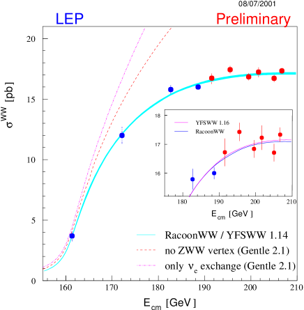
Figure 1: Feynman graphs (left) and measured cross-section (right) for the pair production of W bosons.

As has been measured by the LEP experiments, all three diagrams are needed to describe the data. This can be seen on the right of Fig. 1. Using only the single Abelian graph (the neutrino exchange) or neglecting the non-Abelian Z exchange graph, data and theory disagree. But still the contribution of the graphs could differ from the Standard Model prediction, and therefore a more sophisticated method is performed to analyze the non-Abelian gauge sector.

To study possible other contributions, the Lagrangian for the VWW vertex (V=Z,$\gamma$) can be written in the most general Lorentz invariant form $\!{}^{{\bf?}}$

$$i\mathcal{L}^{WWV}/g_{WWV} = {\color[rgb]{0,0,0}g_{1}^{V}}\left(W_{\mu\nu}^{\dagger}W^{\mu}V^{\nu}-W_{\mu}^{\dagger}V_{\nu}W^{\mu\nu}\right)+{\color[rgb]{0,0,0}\kappa_{V}}W_{\mu}^{\dagger}W_{\nu}V^{\mu\nu}$$

$$+ \frac{\color[rgb]{0,0,0}\lambda_{V}}{m_{W}^{2}}W^{\dagger}_{\mu\nu}W^{\nu}_{\rho}V^{\rho\mu}+C{\color[rgb]{0,0,0}/}+P{\color[rgb]{0,0,0}/}+C{\color[rgb]{0,0,0}/}P{\color[rgb]{0,0,0}/},$$

where C, P and CP-violating terms are not shown and assumed to vanish in the following discussion. To further reduce the parameter set from six to three free couplings, firstly U(1)_em gauge invariance is required, fixing the charge of the W boson to $q_{\rm W}=\pm 1$, which is equivalent to $g_{1}^{\gamma}=1$. Secondly, the requirement of SU(2)${}_{\rm L}\times$U(1)_Y symmetry of the Lagrangian leads to the two constraints $\kappa_{{\rm Z}}=g_{1}^{{\rm Z}}-(\kappa_{\gamma}-1)\tan^{2}\theta_{\rm W}$ and $\lambda_{{\rm Z}}=\lambda_{\gamma}$. The three parameters left are $g_{1}^{{\rm Z}}$, $\kappa_{\gamma}$ and $\lambda_{\gamma}$. In the Standard Model, their values are predicted to be $g_{1}^{{\rm Z}}=1$, $\kappa_{\gamma}=1$ and $\lambda_{\gamma}=0$. Often one finds in the literature also the differences to the Standard Model expectations: $\Delta g_{1}^{{\rm Z}}=g_{1}^{{\rm Z}}-1$ and $\Delta\kappa_{\gamma}=\kappa_{\gamma}-1$.

The couplings are not only accessible in W pair production, but also in single W and single photon production, which also involve the $\gamma$WW vertex, as can be seen from Fig. 2. The W pair production is most sensitive to the couplings $g_{1}^{{\rm Z}}$ and $\lambda_{\gamma}$, and its sensitivity to $\kappa_{\gamma}$ is comparable to the single W production, which in turn is most sensitive to $\kappa_{\gamma}$. From all processes, the single photon production is least sensitive.

single W production

single $\gamma$ production

Figure 2: Other processes that are used in the determination of the VWW couplings.

Deviations from the couplings as they are predicted by the Standard Model would lead to changes of the total cross section, of the production and decay angles and of the average polarization of the bosons.

In the W pair production process, all information about production and decay is contained in five variables: The production angle $\theta_{{\rm W}^{-}}$ of the ${\rm W}^{-}$, the polar and azimuthal angles $\theta,\phi$ of the decay products in the rest frame of the decaying ${\rm W}^{-}$ and ${\rm W}^{+}$ relative to the W flight direction. If a W decays into a charged lepton and a neutrino, $\theta$ and $\phi$ are taken from the charged lepton, and if a W decays into two quarks, the angles are symmetrized to compensate the missing charge determination. The distributions of $\cos\theta_{l}$, $\phi_{l}$ and $\cos\theta_{{\rm W}^{-}}$ in the semileptonic case are shown in Fig. 3 as they have been measured by the L3 experiment and together with the expectations for $g_{1}^{{\rm Z}}=0,1,2$. From the shape of these distributions and the total rate, constraints on the value of the couplings are derived.

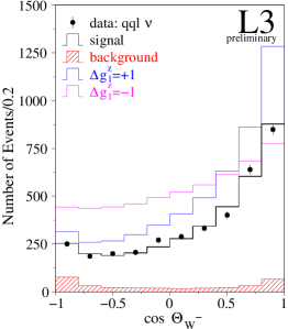
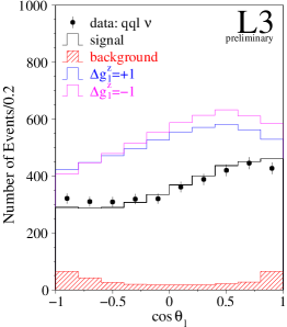
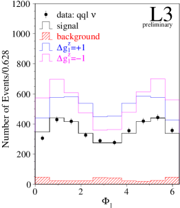
Figure 3: Distribution of the production angle of the W boson and of the decay angles of the lepton in the rest frame of the decaying W in the semileptonic case. The angles for the quarks are not shown.

The shape of the $\cos\theta_{{\rm W}^{-}}$ distribution shows stronger distortions than the shape of the $\cos\theta_{l}$ and $\phi_{l}$ distributions, if the couplings are changed. Therefore, a reliable calculation of these distributions is necessary. Until recently, the theory error was 2% on the rate and larger for the differential distributions like $\cos\theta_{{\rm W}^{-}}$, thus deteriorating the measurement of the gauge couplings. By using the predictions from the newly developed Monte Carlo generators YFSWW3 $\!{}^{{\bf?}}$ and RacoonWW $\!{}^{{\bf?}}$, a theory error of .5% on $\lambda_{\gamma}$ has been achieved$\!{}^{{\bf?}}$. The two generators take into account $\mathcal{O}(\alpha)$-corrections, i. e. diagrams with internal and external photon lines, in the Leading Pole Approximation (LPA) and the Double Pole Approximation DPA, respectively. Some example diagrams of these corrections are shown in Fig. 4.

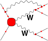
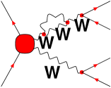
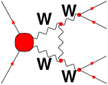
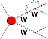
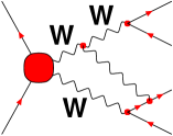
Figure 4: Some example diagrams for $\mathcal{O}(\alpha)$corrections.

By using the predictions from YSFWW3, measurements of the couplings are performed by each experiment, and combined with a log-likelihood method $\!{}^{{\bf?},{\bf?}}$. The likelihood curves of the combined fit are shown in Fig. 5. The measurement of $\kappa_{\gamma}$ agrees within two standard deviations with the Standard Model, and both $\lambda_{\gamma}$ and $g_{1}^{{\rm Z}}$ agree within one standard deviation with the Standard Model. The fitted values with the errors corresponding to $\Delta L=0.5$ are$\!{}^{{\bf?}}$:

$$g_{1}^{{\rm Z}}=0.990^{+0.023}_{-0.024}\hskip 28.45274pt\kappa_{\gamma}=0.896^{+0.058}_{-0.056}\hskip 28.45274pt\lambda_{\gamma}=-0.023^{+0.025}_{-0.023}$$

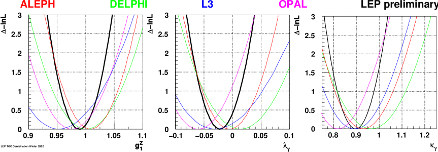
Figure 5: Result of the triple gauge coupling fit.

For this combination, both the L3 and OPAL experiments did not submit the $\rm e^{+}e^{-}\rightarrow W^{+}W^{-}\rightarrow\;$$\rm q_{1}\bar{q}_{2}q_{3}\bar{q}_{4}$ channel. By adding these channels, the statistical accuracy of the measurement will improve. As far as systematic uncertainties are concerned, the $\mathcal{O}(\alpha)$ corrections are the largest correlated ones ($\pm 0.039$ on $\kappa_{\gamma}$, $\pm 0.015$ on $\lambda_{\gamma}$ and $\pm 0.015$ on $g_{1}^{{\rm Z}}$). For the result shown above, they have been set to the full difference between the Monte Carlo prediction with and without $\mathcal{O}(\alpha)$ corrections. More refined numbers will be used in the future, but are not available yet. Also, updates on the fits of higher dimensionality relating two or three couplings are planned.

2 Couplings of three neutral bosons

Figure 6: Couplings of three neutral bosons: Anomalous vertices.

Couplings of three neutral bosons do not exist in the Standard Model. By imposing only Lorentz and U(1)_em invariance, and for final states with equal bosons Bose symmetry, one ends up with possible anomalous vertices shown in Fig. 6. The corresponding Lagrangians $\!{}^{{\bf?},{\bf?}}$ describing these anomalous vertices are

$$\begin{array}[]{rcl}\mathcal{L}_{NP}^{VZZ}=\frac{e}{m_{Z}^{2}}\Bigl{[}&-&{\color[rgb]{0,0,0}f_{4}^{V}}(\partial_{\mu}V^{\mu\beta})Z_{\alpha}(\partial^{\alpha}Z_{\beta})+{\color[rgb]{0,0,0}f_{5}^{V}}(\partial^{\sigma}V_{\sigma\mu})\tilde{Z}^{\mu\beta}Z_{\beta}\Bigr{]}\\ \mathcal{L}_{NP}^{VZ\gamma}=\frac{e}{m_{Z}^{2}}\Bigl{[}&-&{\color[rgb]{0,0,0}h_{1}^{V}}(\partial^{\sigma}V_{\sigma\mu})Z_{\beta}F^{\mu\beta}-{\color[rgb]{0,0,0}h_{3}^{V}}(\partial_{\sigma}V^{\sigma\rho})Z^{\alpha}\tilde{F}_{\rho\alpha}\\ &-&\frac{{\color[rgb]{0,0,0}h_{2}^{V}}}{m_{Z}^{2}}[\partial_{\alpha}\partial_{\beta}(\Box+m_{V}^{2})V_{\mu}]Z^{\alpha}F^{\mu\beta}+\frac{{\color[rgb]{0,0,0}h_{4}^{V}}}{2m_{Z}^{2}}[(\Box+m_{V}^{2})\partial^{\sigma}V^{\rho\alpha}]Z_{\sigma}\tilde{F}_{\rho\alpha}\Bigr{]},\end{array}$$

with $\tilde{V}_{\mu\nu}=\nicefrac{{1}}{{2}}\;\epsilon_{\mu\nu\rho\sigma}V^{\rho\sigma}$ and $V={\rm Z},\gamma$. The Lagrangians are of higher order than those for the gauge couplings of the W boson, so that one would expect either to detect deviations more easily with the W boson couplings or the scale of New Physics (which is artificially set to $m_{Z}$ in the above formulae) to be close. The couplings $f_{4}^{V}$, $h_{1}^{V}$ and $h_{2}^{V}$ are CP violating, whereas the couplings $f_{5}^{V}$, $h_{3}^{V}$ and $h_{4}^{V}$ conserve CP. One interesting option for the future, which has not been followed yet, is to relate the couplings through SU(2)${}_{\rm L}\times$U(1)_Y symmetry $\!{}^{{\bf?}}$. This relates the couplings from the Z$\gamma$ and from the ZZ final state in the following way: ${\color[rgb]{0,0,0}f_{5}^{\rm V}}={\color[rgb]{0,0,0}h_{3}^{\rm V}}\tan\theta_{\rm W}$ and ${\color[rgb]{0,0,0}f_{4}^{\rm V}}={\color[rgb]{0,0,0}h_{1}^{\rm V}}\tan\theta_{\rm W}$.

The measurement of the $f$ couplings proceeds by selecting events from all visible ZZ final states and then reweighting the distributions for different values of the anomalous couplings $f_{4,5}^{{\rm Z},\gamma}$. In the presence of anomalous couplings, the total cross-section, the production angle of the Z boson and the average polarization of the Z bosons would change. In Fig. 7 the distribution of the Z boson production angle $\cos\theta_{\rm Z}$ as predicted by the Standard Model and for $f_{5}^{\rm Z}=\pm 1.5$ is compared to the data, as they have been measured by the DELPHI experiment.

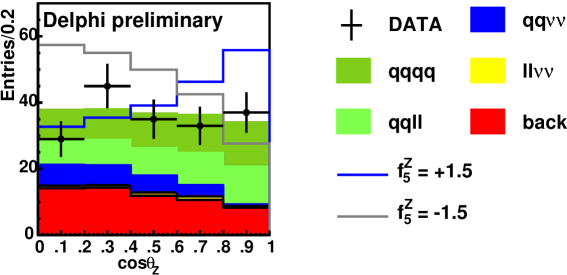
Figure 7: ZZ production angle measured by DELPHI compared to the Standard Model prediction and $f_{5}^{\rm Z}=\pm 1.5$.

Since in all LEP data no evidence for the presence of anomalous $f$ couplings has been found, limits at the 95% confidence level are set. These limits are derived either one-dimensional by fixing all other couplings to zero, or two-dimensional by fitting couplings with the same CP behavior at the same time. The one-dimensional limits are$\!{}^{{\bf?}}$:

$$-0.17<f_{4}^{\gamma}<0.19\hskip 28.45274pt-0.31<f_{4}^{Z}<0.28\hskip 28.45274pt-0.36<f_{5}^{\gamma}<0.40\hskip 28.45274pt-0.36<f_{5}^{Z}<0.39$$

For the $h$-couplings, events of the reactions $\rm e^{+}e^{-}\rightarrow Z/\gamma^{*}\rightarrow\;\rm q\bar{q}\gamma$ and $\rm e^{+}e^{-}\rightarrow Z/\gamma^{*}\rightarrow\;\nu\bar{\nu}\gamma$ are selected. The photon energy $E_{\gamma}$, the angle $\cos\alpha_{\gamma-{\rm jet}}$ between the photon and the nearest jet, and the photon production angle $\cos\theta_{\gamma}$ are sensitive to the anomalous couplings. In Fig. 8, distributions of these variables from the OPAL experiment are shown, for the Standard Model prediction and for $h_{3}^{\gamma}=\pm 0.5$. No evidence for anomalous $h$ couplings has been found, and one- and two-dimensional limits are derived. The one-dimensional limits are$\!{}^{{\bf?}}$:

$$\begin{array}[]{llll}-0.056<h_{1}^{\gamma}<0.055&-0.045<h_{2}^{\gamma}<0.025&-0.130<h_{1}^{Z}<0.130&-0.078<h_{2}^{Z}<0.071\\ -0.049<h_{3}^{\gamma}<0.008&-0.002<h_{4}^{\gamma}<0.034&-0.200<h_{3}^{Z}<0.070&-0.050<h_{4}^{Z}<0.120\end{array}$$

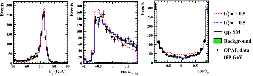
Figure 8: Distributions of $E_{\gamma}$, $\cos\alpha_{\gamma-{\rm jet}}$ and $\cos\theta_{\gamma}$ for the $\rm q\bar{q}\gamma$ final state. Predictions from the Standard Model and for $h_{3}^{\gamma}=\pm 0.5$ are compared to the data.

3 Quartic boson self couplings

Starting from U(1)_em gauge invariance and requiring a custodial SU(2)_c symmetry, genuine quartic couplings (i. e. quartic couplings that are not introduced to counteract the trilinear gauge couplings to achieve SU(2)${}_{\rm L}\times$U(1)_Y symmetry) arise through the Lagrangians$\!{}^{{\bf?},{\bf?}}$

$$\begin{array}[]{ll}\mathcal{L}_{0}=-\frac{e^{2}}{16}\frac{{\color[rgb]{0,0,0}a_{0}^{W,Z}}}{{\color[rgb]{0,0,0}\Lambda}^{2}}F^{\mu\nu}F_{\mu\nu}\vec{W}^{\alpha}\vec{W}_{\alpha}&WW\gamma\gamma,ZZ\gamma\gamma\\ \mathcal{L}_{c}=-\frac{e^{2}}{16}\frac{{\color[rgb]{0,0,0}a_{c}^{W,Z}}}{{\color[rgb]{0,0,0}\Lambda}^{2}}F^{\mu\alpha}F_{\mu\beta}\vec{W}^{\beta}\vec{W}_{\alpha}&WW\gamma\gamma,ZZ\gamma\gamma\\ \mathcal{L}_{n}=-\frac{e^{2}}{16}\frac{{\color[rgb]{0,0,0}a_{n}}}{{\color[rgb]{0,0,0}\Lambda}^{2}}\vec{W}_{\mu\alpha}\cdot(\vec{W}_{\nu}\times\vec{W}^{\alpha})F^{\mu\nu}&WWZ\gamma\end{array}$$

Figure 9: Anomalous contributions to quartic gauge couplings.

The couplings $a_{0}$ and $a_{c}$ conserve CP, the coupling $a_{n}$ violates CP. Figure 9 shows the relationship between the vertices and the anomalous couplings. In principle, the couplings of the W can be different from the couplings of the Z, hence the different superscripts.

These couplings are accessible either through boson fusion with two bosons in the final state or through the production of three gauge bosons. The fusion processes become important only at Linear Collider energies and are negligible at LEP. Recent results$\!{}^{{\bf?}}$ from L3 for the process $\rm e^{+}e^{-}\!\!\rightarrow W^{+}W^{-}\gamma$, which would dominate a possible LEP combination for $a^{\rm W}_{0}$, $a^{\rm W}_{c}$ and $a_{n}$, allow to set the following limits at 95% CL:

$$\begin{array}[]{ccc}-0.02<{\color[rgb]{0,0,0}a^{\rm W}_{0}}/{\color[rgb]{0,0,0}\Lambda}^{2}\cdot\mbox{GeV}^{2}<0.02&-0.05<{\color[rgb]{0,0,0}a^{\rm W}_{c}}/{\color[rgb]{0,0,0}\Lambda}^{2}\cdot\mbox{GeV}^{2}<0.03&-0.14<{\color[rgb]{0,0,0}a_{n}}/{\color[rgb]{0,0,0}\Lambda}^{2}\cdot\mbox{GeV}^{2}<0.13\end{array}$$

The energy of the least energetic photon in the process $\rm e^{+}e^{-}\!\!\rightarrow Z\gamma\gamma$ is especially sensitive to the presence of anomalous quartic couplings and used as a test distribution. Since no evidence for such couplings is found, limits are set at 95% CL by L3 as$\!{}^{{\bf?}}$:

$$\begin{array}[]{cc}-0.02<{\color[rgb]{0,0,0}a^{\rm Z}_{0}}/{\color[rgb]{0,0,0}\Lambda}^{2}\cdot\mbox{GeV}^{2}<0.03&-0.07<{\color[rgb]{0,0,0}a^{\rm Z}_{c}}/{\color[rgb]{0,0,0}\Lambda}^{2}\cdot\mbox{GeV}^{2}<0.05\end{array}$$

References

References

[1]K. Hagiwara, R. D. Peccei, D. Zeppenfeld and
K. Hikasa,
Nucl. Phys. B 282, 253 (1987)
[2]S. Jadach et al., Comp. Phys. Comm.140, 432 (2001)
[3]A. Denner et al., Nucl. Phys. B 560, 33 (1999)
[4]R. Brunelière et al., hep-ph/0201304, (2002)
[5]J. Alcaraz, L3 internal note 2718, (2001)
[6]The LEP Collaborations ALEPH, DELPHI, L3, OPAL,
and the LEP TGC Working Group, LEPEWWG/TGC/2002-01, (2002),
http://lepewwg.web.cern.ch/LEPEWWG/lepww/tgc/
[7]G. J. Gounaris et al., Phys. Rev. D 61, 073013 (2000)
[8]J. Alcaraz, Phys. Rev. D 65, 075020 (2002)
[9]G. Bélanger and F. Boudjema, Phys. Lett. B 288, 210 (1992)
[10]W. J. Stirling and Ghadir Abu Leil,
J. Phys. G 21, 517 (1995)
[11]L3 Collaboration, Phys. Lett. B 527/1-2, 29 (2002)