Search for mSUGRA in single-electron events with jets and large missing transverse energy in $p\overline{p}$ collisions at $\sqrt{s}=1.8$ TeV

Abstract

We describe a search for evidence of minimal supergravity (mSUGRA) in $92.7\;\rm{pb}^{-1}$ of data collected with the DØ detector at the Fermilab Tevatron $p\overline{p}$ collider at $\sqrt{s}=1.8\;{\rm TeV}$. Events with a single electron, four or more jets, and large missing transverse energy were used in this search. The major backgrounds are from $W$+jets, misidentified multijet, $t\overline{t}$, and $WW$ production. We observe no excess above the expected number of background events in our data. A new limit in terms of mSUGRA model parameters is obtained.

Abstract

I INTRODUCTION

The standard model (SM) has been a great achievement in particle physics. A large number of experimental results have confirmed many features of the theory to a high degree of precision. However, the SM is theoretically unsatisfactory, and it poses many questions and problems [3, 4]. The most notable ones are the fine-tuning problem of the SM Higgs self-interaction through fermion loops [5] and the unknown origin of electroweak symmetry breaking (EWSB).  Supersymmetry (SUSY) [6] incorporates an additional symmetry between fermions and bosons, and offers a solution to the fine-tuning problem and a possible mechanism for EWSB.

SUSY postulates that for each SM degree of freedom, there is a corresponding SUSY degree of freedom. This results in a large number of required supersymmetric particles (sparticles), and at least two Higgs doublets in the theory. A new quantum number, called $R$-parity [7], is used to distinguish between SM particles and sparticles. All SM particles have $R$-parity $+1$ and sparticles have $R$-parity $-1$. The simplest extension to the SM, the minimal supersymmetric standard model (MSSM), respects the same $\mbox{SU(3)}\otimes\mbox{SU(2)}\otimes\mbox{U(1)}$ gauge symmetries as does the SM. SUSY must be a broken symmetry. Otherwise we would have discovered supersymmetric particles of the same masses as their SM partners. A variety of models have been proposed for SUSY breaking. One of these, the minimal supergravity (mSUGRA) model, postulates that gravity is the communicating force from the SUSY breaking origin at a high mass scale to the electroweak scale, which is accessible to current high energy colliders. The mSUGRA model is described in detail in Ref. [8]. It can be characterized by four parameters and a sign: a common scalar mass ($m_{0}$), a common gaugino mass ($m_{1/2}$), a common trilinear coupling value ($A_{0}$), the ratio of the vacuum expectation values of the two Higgs doublets ($\tan\beta$), and the sign of $\mu$, where $\mu$ is the Higgsino mass parameter.

In this analysis, $R$-parity is assumed to be conserved. This implies that sparticles must be pair-produced in $p\overline{p}$ collisions. The sparticles can decay directly, or via lighter sparticles, into final states that contain SM particles and the lightest supersymmetric particles (LSPs), which must be stable. Because the LSP interacts extremely weakly, it escapes detection and leaves a large imbalance in transverse energy (${\hbox{$E$\kern-6.00006pt\lower-0.43057pt\hbox{/}}}_{T}$) in the event. We assume that the lightest neutralino ($\widetilde{\chi}_{1}^{0}$) is the LSP, and that $A_{0}=0$ and $\mu<0$. We fix $\tan\beta=3$ and perform the search in the $m_{1/2}$–$m_{0}$ plane.

Most recently, searches for mSUGRA signatures have been performed at LEP and the Tevatron. At DØ, dilepton+${\hbox{$E$\kern-6.00006pt\lower-0.43057pt\hbox{/}}}_{T}$ [9] and jets+${\hbox{$E$\kern-6.00006pt\lower-0.43057pt\hbox{/}}}_{T}$ [10] final states have been examined for possible mSUGRA effects. This report describes a search in the final state containing a single isolated electron, four or more jets, and large ${\hbox{$E$\kern-6.00006pt\lower-0.43057pt\hbox{/}}}_{T}$. One of the possible mSUGRA particle-production processes which results in such a final state is shown in Fig. 1. The search is particularly sensitive to the moderate $m_{0}$ region where charginos and neutralinos decay mostly into SM $W$ and/or $Z$ bosons which have large branching fractions to jets. It also complements our two previous searches since the signatures are orthogonal to one another.

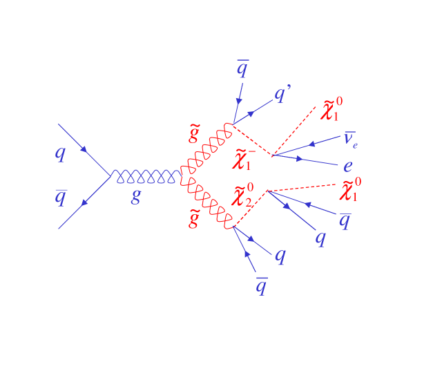
FIG. 1.: Feynman diagram for gluino pair production and decay to an electron, multijets, and produce ${\hbox{$E$\kern-6.00006pt\lower-0.43057pt\hbox{/}}}_{T}$. The three-body decays are in fact cascade decays in which off-shell particles or sparticles are produced.

II THE DØ DETECTOR

DØ is a multipurpose detector designed to study $p\overline{p}$ collisions at the Fermilab Tevatron Collider. The work presented here is based on approximately $92.7\;\rm{pb}^{-1}$ of data recorded during the 1994–1996 collider runs. A full description of the detector can be found in Ref. [11]. Here, we describe briefly the properties of the detector that are relevant for this analysis.

The detector was designed to have good electron and muon identification capabilities and to measure jets and ${\hbox{$E$\kern-6.00006pt\lower-0.43057pt\hbox{/}}}_{T}$ with good resolution. The detector consists of three major systems: a non-magnetic central tracking system, a uranium/liquid-argon calorimeter, and a muon spectrometer. A cut-away view of the detector is shown in Fig. 2.

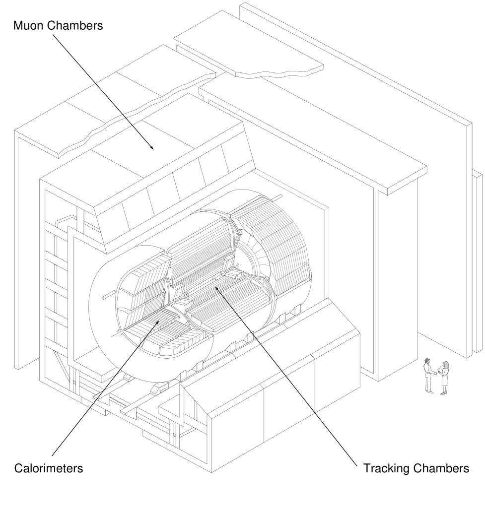
FIG. 2.: Cut away isometric view of the DØ detector.

The central detector (CD) consists of four tracking subsystems: a vertex drift chamber, a transition radiation detector, a central drift chamber, and two forward drift chambers. It measures the trajectories of charged particles and can discriminate between singly-charged particles and $e^{+}e^{-}$ pairs from photon conversions through the ionization measured along their tracks. It covers the pseudorapidity [12] region $|\eta_{\rm d}|<3.2$.

The calorimeter is divided into three parts: the central calorimeter (CC) and the two end calorimeters (EC), each housed in its own steel cryostat, which together cover the pseudorapidity range $|\eta_{\rm d}|<4.2$. Each calorimeter consists of an inner electromagnetic (EM) section, a fine hadronic (FH) section, and a coarse hadronic (CH) section. Between the CC and the EC is the inter-cryostat detector (ICD), which consists of scintillator tiles. The EM portion of the calorimeters is 21 radiation lengths deep and is divided into four longitudinal segments (layers). The hadronic portions are 7–9 nuclear interaction lengths deep and are divided into four (CC) or five (EC) layers. The calorimeters are segmented transversely into pseudoprojective towers of $\Delta\eta\times\Delta\phi=0.1\times 0.1$. The third layer of the EM calorimeter, where most of the EM shower energy is expected, is segmented twice as finely in both $\eta$ and $\phi$, with cells of size $\Delta\eta\times\Delta\phi$ = $0.05\times 0.05$. The energy resolution for electrons is $\sigma(E)/E=15\%/\sqrt{E(\rm{GeV})}\oplus 0.4\%$. For charged pions, the resolution is $50\%/\sqrt{E(\rm{GeV})}$ and for jets $80\%/\sqrt{E(\rm{GeV})}$. The resolution in ${\hbox{$E$\kern-6.00006pt\lower-0.43057pt\hbox{/}}}_{T}$ is $1.08\;{\rm GeV}+0.019\cdot\sum E_{T}({\rm GeV})$, where $\sum E_{T}$ is the scalar sum of the transverse energies in all calorimeter cells.

The wide angle muon system (WAMUS), which covers $|\eta_{\rm d}|<2.5$, is also used in this analysis. The system consists of four planes of proportional drift tubes in front of magnetized iron toroids with a magnetic field of 1.9 T and two groups of three planes of proportional drift tubes behind the toroids. The magnetic field lines and the wires in the drift tubes are transverse to the beam direction. The muon momentum $p$ is measured from the muon’s angular bend in the magnetic field of the iron toroids, with a resolution of $\sigma(1/p)=0.18(p-2\;{\rm GeV})/p^{2}\oplus 0.003\;{\rm GeV}^{-1}$, for $p>4.0\;{\rm GeV}$.

A separate synchrotron, the Main Ring, lies above the Tevatron and goes through the CH calorimeter. During data-taking, it is used to accelerate protons for antiproton production. Particles lost from the Main Ring can deposit significant energy in the calorimeters, increasing the instrumental background. We reject much of this background at the trigger level by not accepting events during beam injection into the Main Ring, when losses are largest.

III EVENT SELECTION

Event selection at DØ is performed at two levels: online selection at the trigger level and offline selection at the analysis level. The algorithms to reconstruct the physical objects (electron, muon, jet, ${\hbox{$E$\kern-6.00006pt\lower-0.43057pt\hbox{/}}}_{T}$) as well as their identification at the online and offline levels are described in Ref. [13]. We summarize below the selections pertaining to this analysis.

A Triggers

The DØ trigger system reduces the event rate from the beam crossing rate of 286 kHz to approximately 3–4 Hz, at which the events are recorded on tape. For most triggers (and those we use in this analysis) we require a coincidence in hits between the two sets of scintillation counters located in front of each EC (level 0). The next stage of the trigger (level 1) forms fast analog sums of the transverse energies in calorimeter trigger towers. These towers have a size of $\Delta\eta\times\Delta\phi=0.2\times 0.2$, and are segmented longitudinally into EM and FH sections. The level 1 trigger operates on these sums along with patterns of hits in the muon spectrometer. A trigger decision can be made between beam crossings (unless a level 1.5 decision is required, as described below). After level 1 accepts an event, the complete event is digitized and sent to the level 2 trigger, which consists of a farm of 48 general-purpose processors. Software filters running in these processors make the final trigger decision.

The triggers are defined in terms of combinations of specific objects required in the level 1 and level 2 triggers. These elements are summarized below. For more information, see Refs. [11, 13].

To trigger on electrons, level 1 requires that the transverse energy in the EM section of a trigger tower be above a programmed threshold. The level 2 electron algorithm examines the regions around the level 1 towers that are above threshold, and uses the full segmentation of the EM calorimeter to identify showers with shapes consistent with those of electrons. The level 2 algorithm can also apply an isolation requirement or demand that there be an associated track in the central detector.

For the later portion of the run, a “level 1.5” processor was also available for electron triggering. In this processor, each EM trigger tower above the level 1 threshold is combined with the neighboring tower of the highest energy. The hadronic portions of these two towers are also combined, and the ratio of EM transverse energy to total transverse energy in the two towers is required to be $>0.85$. The use of a level 1.5 electron trigger is indicated in the tables below as an “EX” tower.

The level 1 muon trigger uses the pattern of drift tube hits to provide the number of muon candidates in different regions of the muon spectrometer. A level 1.5 processor can also be used to put a $p_{T}$ requirement on the candidates (at the expense of slightly increased dead time). At level 2, the fully digitized event is available, and the first stage of the full event reconstruction is performed. The level 2 muon algorithm can also require the presence of energy deposition in the calorimeter consistent with that from a muon.

For a jet trigger, level 1 requires that the sum of the transverse energies in the EM and hadronic sections of a trigger tower be above a programmed threshold. Level 2 then sums calorimeter cells around the identified towers (or around the $E_{T}$-weighted centroids of the large tiles) in cones of a specified radius $\Delta R=\sqrt{\Delta\eta^{2}+\Delta\phi^{2}}$, and imposes a threshold on the total transverse energy.

The ${\hbox{$E$\kern-6.00006pt\lower-0.43057pt\hbox{/}}}_{T}$ in the calorimeter is computed both at level 1 and level 2. For level 1, the vertex $z$ position is assumed to be at the center of the detector, while for level 2, the vertex $z$ position is determined from the relative timing of hits in the level 0 scintillation counters.

The trigger requirements used for this analysis are summarized in Table I. Runs taken during 1994–1995 (Run 1b) and during the winter of 1995–1996 (Run 1c) were used, and only the triggers “ELE_JET_HIGH” and “ELE_JET_HIGHA” in the table were used to conduct this search for mSUGRA. The “EM1_EISTRKCC_MS” trigger was used for background estimation. As mentioned above, these triggers do not accept events during beam injection into the main ring. In addition, we do not use events which were collected when a Main Ring bunch passed through the detector or when losses were registered in monitors around the Main Ring. Several bad runs resulting from hardware failure were also rejected. The “exposure” column in Table I takes these factors into account.

TABLE I.: Triggers used during Run 1b and Run 1c. “Exposure” gives the effective integrated luminosity for each trigger, taking into account the Main Ring vetoes and bad runs.

Trigger Name	Exposure	Level 1	Level 2	Run
	($\rm{pb}^{-1}$)			period
EM1_EISTRKCC_MS	82.9	1 EM tower, $E_{T}>10\;\rm{GeV}$	1 isolated $e$, $E_{T}>20\;\rm{GeV}$	Run 1b
		1 EX tower, $E_{T}>15\;\rm{GeV}$	$\mbox{\mbox{${\hbox{$E$\kern-6.00006pt\lower-0.43057pt\hbox{/}}}_{T}^{\rm cal}$}}>15\;\rm{GeV}$
		1 EM tower, $E_{T}>12\;\rm{GeV}$, $|\eta|<2.6$	1 $e$, $E_{T}>15\;\rm{GeV}$, $|\eta|<2.5$
ELE_JET_HIGH	82.9	2 jet towers, $E_{T}>5\;\rm{GeV}$, $|\eta|<2.0$	2 jets ($\Delta R=0.3$), $E_{T}>10\;\rm{GeV}$, $|\eta|<2.5$	Run 1b
			$\mbox{\mbox{${\hbox{$E$\kern-6.00006pt\lower-0.43057pt\hbox{/}}}_{T}^{\rm cal}$}}>14\;\rm{GeV}$
ELE_JET_HIGH	0.89	ditto	ditto	Run 1c
		1 EM tower, $E_{T}>12\;\rm{GeV}$, $|\eta|<2.6$	1 $e$, $E_{T}>17\;\rm{GeV}$, $|\eta|<2.5$
ELE_JET_HIGHA	8.92	2 jet towers, $E_{T}>5\;\rm{GeV}$, $|\eta|<2.0$	2 jets ($\Delta R=0.3$), $E_{T}>10\;\rm{GeV}$, $|\eta|<2.5$	Run 1c
			$\mbox{\mbox{${\hbox{$E$\kern-6.00006pt\lower-0.43057pt\hbox{/}}}_{T}^{\rm cal}$}}>14\;\rm{GeV}$

B Object Identification

1 Electrons

Electron identification is based on a likelihood technique. Candidates are first identified by finding isolated clusters of energy in the EM calorimeter with a matching track in the central detector. We then cut on a likelihood constructed from the following five variables:

• a $\chi^{2}$ from a covariance matrix that checks the consistency of the shape of a calorimeter cluster with that expected of an electron shower;

• an electromagnetic energy fraction, defined as the ratio of the portion of the energy of the cluster found in the EM calorimeter to its total energy;

• a measure of consistency between the trajectory in the tracking chambers and the centroid of energy cluster (track match significance);

• the ionization deposited along the track $dE/dx$;

• a measure of the radiation pattern observed in the transition radiation detector (TRD). (This variable is used only for CC EM clusters because the TRD does not cover the forward region [11].)

To a good approximation, these five variables are independent of each other.

High energy electrons in mSUGRA events tend to be isolated. Thus, we use the additional restriction:

$${E_{\rm{tot}}(0.4)-E_{\rm{EM}}(0.2)\over E_{\rm{EM}}(0.2)}<0.1,$$ (1)

where $E_{\rm{tot}}(0.4)$ is the energy within $\Delta R<0.4$ of the cluster centroid ($\Delta R=\sqrt{\Delta\eta^{2}+\Delta\phi^{2}}$) and $E_{\rm{EM}}(0.2)$ is the energy in the EM calorimeter within $\Delta R<0.2$. We denote this restriction the “isolation requirement.”

The electron identification efficiency, $\varepsilon^{e}_{\rm id}$, is measured using the $Z\rightarrow ee$ data. Since only CC ($|\eta^{e}_{\rm d}|<1.1$) and EC ($1.5<|\eta^{e}_{\rm d}|<2.5$) regions are covered by EM modules, electron candidates are selected and their identification efficiencies are measured in these two regions. An electron is considered a “probe” electron if the other electron in the event passes a strict likelihood requirement. This gives a clean and unbiased sample of electrons. We construct the invariant mass spectrum of the two electron candidates and calculate the number of background events, which mostly come from Drell-Yan production and misidentified jets, inside a $Z$ boson mass window. After background subtraction, the ratio of the number of events inside the $Z$ boson mass window before and after applying the likelihood and isolation requirements to each probe electron, gives $\varepsilon^{e}_{\rm id}$.

The $\varepsilon^{e}_{\rm id}$ is a function of jet multiplicity in the event. The presence of jets reduces $\varepsilon^{e}_{\rm id}$ primarily due to the isolation requirement and reduced tracking efficiency. However, with a larger numbers of jets ($\geq 3$) in the event, the efficiency of locating the correct hard-scattering vertex increases. The two effects compensate each other for events with high jet multiplicity [14]. The electron identification efficiencies used in this analysis are obtained from $Z\rightarrow ee$ data with at least two jets and are given in Table II.

Sometimes a jet with very similar characteristics to an electron can pass the electron identification selection, and result in a fake electron. The effect of fake electrons is discussed in section V A.

2 Jets

Jets are reconstructed in the calorimeter using a fixed-size cone algorithm with $\Delta R=0.5$. A jet that originates from a quark or a gluon deposits a large fraction of its energy in the FH part of the calorimeter, and so we identify jets through the fractional energy in the EM and CH parts of the calorimeter. We require the fraction of the total jet energy deposited in the EM section of the calorimeter (emf ) to be between 0.05 and 0.95 for high energy jets ($E^{j}_{T}>35\;{\rm GeV}$), and the fraction of the total jet energy deposited in the CH section of the calorimeter (chf ) to be less than 0.4. Because electronic and uranium noise is generally of low energy, the lower bound of the emf  requirement is raised gradually for lower energy jets in the CC. (It is 0.2 for CC jets with $E^{j}_{T}\approx 15\;{\rm GeV}$.) Because there is no electromagnetic coverage in the ICR, we do not apply a lower bound cut on emf  in that region.

TABLE II.: Electron ID efficiencies used in this analysis.

Detector Region	CC	EC
$\varepsilon^{e}_{\rm id}$	$0.674\pm 0.039$	$0.242\pm 0.075$

A multijet data sample corrected for detector noise is used to measure the jet identification efficiency, $\varepsilon^{j}_{\rm id}$. The efficiency is a function of $E^{j}_{T}$, and is parametrized as in Eq. 2, with the fitted values of the parameters listed in Table III.

$$\varepsilon^{j}_{\rm id}=p_{0}+p_{1}\times E^{j}_{T}+p_{2}\times(E^{j}_{T})^{2}.$$ (2)

TABLE III.: Parameters for jet identification efficiency as defined in Eq. 2.

Fiducial Region	$E^{j}_{T}\;(\rm{GeV})$	$p_{0}$	$p_{1}\;(\rm{GeV}^{-1})$	$p_{2}\;(\rm{GeV}^{-2})$
CC	$15$–$27.4$	$0.8994\pm 0.0070$	$(5.04\pm 0.45)\times 10^{-3}$	$(-6.7\pm 1.0)\times 10^{-5}$
($|\eta^{j}_{\rm d}|<1.0$)	$\geq 27.4$	$0.9864\pm 0.0005$	$(2.16\pm 0.57)\times 10^{-5}$	$(-1.90\pm 0.30)\times 10^{-7}$
ICR	$15$–$30.5$	$0.9838\pm 0.0017$	$(9.76\pm 1.33)\times 10^{-4}$	$(-1.76\pm 0.27)\times 10^{-5}$
($1.0<|\eta^{j}_{\rm d}|<1.5$)	$\geq 30.5$	$0.9981\pm 0.0008$	$(-2.27\pm 2.26)\times 10^{-5}$	$(-1.52\pm 1.22)\times 10^{-7}$
EC		$0.9866\pm 0.0004$	$(-3.81\pm 1.05)\times 10^{-5}$	$(-1.15\pm 0.75)\times 10^{-7}$
($1.5<|\eta^{j}_{\rm d}|<2.5$)

3 Muons

To avoid overlapping with the dilepton analysis, we veto events containing isolated muons satisfying all the following criteria:

• The muon has a good track originating from the interaction vertex.

• The muon has pseudorapidity $|\eta^{\mu}_{\rm d}|\leq 2.5$.

• There is a large integrated magnetic field along the muon trajectory ($\int\vec{B}\cdot d\vec{l}\;$). This ensures that the muon traverses enough of the field to give a good $P_{T}$ measurement.

• The energy deposited in the calorimeter along a muon track is at least that expected from a minimum ionizing particle.

• Transverse momentum $p_{T}\geq 4\;\rm{GeV}$.

• The distance in the $\eta-\phi$ plane between the muon and the closest jet is $\Delta R(\mu,j)>0.5$.

4 Event selection

About 1.9 million events passed the ELE_JET_HIGH and the ELE_JET_HIGHA triggers. We require at least one electromagnetic cluster with $E_{T}>18\;{\rm GeV}$ and a track matched to it. The interaction vertex must be within $|z_{v}|<60\;\rm{cm}$. About 600,000 events remain after these selections. Kinematic and fiducial requirements are then applied to select our base data sample. The criteria are listed below, with numbers in the curly brackets specifying the number of events surviving the corresponding requirement.

• One electron in the good fiducial volume ($|\eta^{e}_{\rm d}|<1.1$ or $1.5<|\eta^{e}_{\rm d}|<2.5$) passing restrictive electron identification criteria, and with $E^{e}_{T}>20\;\rm{GeV}$ — {15547}.

• No extra electrons in the good fiducial volume passing “loose” electron identification for $E^{e}_{T}>15\;\rm{GeV}$. The selection criteria for the “loose” electrons are the same as those used for signal electrons in the dilepton analysis, keeping two analyses independent of each other — {15319}.

• $|\eta^{e}|<2.0$ — {13997}.

• No isolated muons — {13980}.

• Four or more jets with $E_{T}^{j}>15\;\rm{GeV}$ and $|\eta^{j}_{\rm d}|<2.5$ — {187}.

• $\mbox{\mbox{${\hbox{$E$\kern-6.00006pt\lower-0.43057pt\hbox{/}}}_{T}$}}>25\;\rm{GeV}$ — {72}.

After these selections the base sample contains 72 events. The major SM backgrounds are from $W+\geq 4$ jets $\rightarrow e+\nu+\geq 4$ jets, $t\overline{t}\rightarrow Wb\;Wb\rightarrow e+\nu+\geq 4$ jets, $WW+\geq 2\;\mbox{jets}\rightarrow e+\nu+\geq 4$ jets, and multijet events in which one of the jets is misidentified as an electron and the jet transverse energies are inaccurately measured to give rise to ${\hbox{$E$\kern-6.00006pt\lower-0.43057pt\hbox{/}}}_{T}$.

IV EVENT SIMULATION

We use pythia [15] to simulate mSUGRA signal and $t\overline{t}$ and $WW$ backgrounds. We check our results and obtain generator-dependent systematic errors using the herwig [16] generator. $W$ boson and associated jet production is generated using vecbos [17] and herwig. The final state partons, which are generated by vecbos as a result of a leading order calculation, are passed through herwig to include the effects of additional radiation and the underlying processes, and to model the hadronization of the final state partons [18].

In order to efficiently search for mSUGRA in a large parameter space and to reduce the statistical error on signal acceptance, we used a fast Monte Carlo program called fmcø [19] to model events in the DØ detector and to calculate the acceptance for any physics process passing our trigger and offline selections. The flow-chart of fmcø is shown in Fig. 3. First, through a jet-reconstruction program, the stable particles that interact in the detector are clustered into particle jets, in a way similar to the clustering of calorimeter cells into jets. However, the generated electrons, if they are not close to a jet ($\Delta R>0.5$ in $\eta-\phi$ space), are considered as the electrons reconstructed in the detector. Otherwise, they are clustered into the jet. The generated muons are considered as the reconstructed muons in the detector. Next, the electrons, jets, muons, and ${\hbox{$E$\kern-6.00006pt\lower-0.43057pt\hbox{/}}}_{T}$ in the events are smeared according to their resolutions determined from data [18]. The offline selections (Sec. III B 4) are applied to the smeared objects. Finally, each passed event is weighted with trigger and identification efficiencies. The outputs of fmcø are an “ntuple” that contains the kinematic characteristics ($E_{T}$, $\eta$, $\phi$, etc.) of every object and a run-summary ntuple that contains the information of trigger efficiency and total acceptance for the process being simulated. The acceptance $A$ is calculated as follows:

$$A=\frac{1}{N_{\rm gen}}\sum_{i}^{N_{\rm pass}}\varepsilon^{\rm total}_{\rm trig}\cdot\varepsilon^{e}_{\rm id}\cdot\varepsilon^{\rm jets}_{\rm id},$$ (3)

where $\varepsilon^{\rm total}_{\rm trig}$ is the overall trigger efficiency, $\varepsilon^{e}_{\rm id}$ is the electron identification efficiency, $\varepsilon^{\rm jets}_{\rm id}$ is the product of jet identification efficiencies of the four leading jets, $N_{\rm gen}$ is the number of generated events, and $N_{\rm pass}$ is the number of events that pass the offline kinematic requirements. The uncertainty on the acceptance, $\delta_{A}$, is calculated as:

$$\delta_{A}=\frac{1}{N_{\rm gen}}\sum_{i}^{N_{\rm pass}}\delta_{\varepsilon},$$ (4)

where $\delta_{\varepsilon}$ comes from the propagation of uncertainties on $\varepsilon^{\rm total}_{\rm trig}$, $\varepsilon^{e}_{\rm id}$, and $\varepsilon^{\rm jets}_{\rm id}$. Since the same electron and jet identification efficiencies, and the same trigger turn-ons are used the error on the acceptance is 100% correlated event-by-event as shown in Eq. 4.

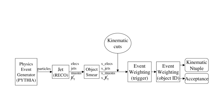
FIG. 3.: Flow-chart of fmcø. Prefix “s_” refers to smeared objects.

Because the signal triggers impose a combination of requirements on the electron, jets, and ${\hbox{$E$\kern-6.00006pt\lower-0.43057pt\hbox{/}}}_{T}$, the overall trigger efficiency has three corresponding components. The efficiency of each component was measured using data. The individual efficiencies are then used to construct the overall trigger efficiency. The details of the measurements and construction are documented in Ref. [14]. Table IV compares the trigger efficiencies of $W+$ jets events measured in data with those simulated using vecbos Monte Carlo. We find that they are in good agreement at each jet multiplicity.

TABLE IV.: Comparison of $\varepsilon^{total}_{trig}$, the total trigger efficiency of ELE_JET_HIGH trigger. The second column lists the efficiencies measured using $W+$ jets data; the third column lists the simulated efficiencies found by putting the vecbos $W+$ jets events through fmcø.

$N_{\rm jet}$	Data	vecbos
$\geq 1$	$0.589\pm 0.019$	$0.579\pm 0.022$
$\geq 2$	$0.826\pm 0.027$	$0.833\pm 0.020$
$\geq 3$	$0.928\pm 0.031$	$0.925\pm 0.016$
$\geq 4$	$0.944\pm 0.037$	$0.957\pm 0.012$

We also compared the acceptance of fmcø with geant [20] and data, and found good agreement for $W+$ jets, $t\overline{t}$, and $WW$ events.

V BACKGROUNDS

A Multijet background

From the ELE_JET_HIGH and ELE_JET_HIGHA triggered data we obtain two sub-samples. For sample 1, we require all offline criteria to be satisfied, except for ${\hbox{$E$\kern-6.00006pt\lower-0.43057pt\hbox{/}}}_{T}$. At small ${\hbox{$E$\kern-6.00006pt\lower-0.43057pt\hbox{/}}}_{T}$ ($<20\;{\rm GeV}$), sample 1 contains contributions mainly from multijet production, where jet energy fluctuations give rise to ${\hbox{$E$\kern-6.00006pt\lower-0.43057pt\hbox{/}}}_{T}$. At large ${\hbox{$E$\kern-6.00006pt\lower-0.43057pt\hbox{/}}}_{T}$ ($>25\;{\rm GeV}$), it has significant contributions from $W+$ jets events, with additional contributions from $t\overline{t}$ production and possibly the mSUGRA signal. For sample 2, we require that the EM object represent a very unlikely electron candidate by applying an “anti-electron” requirement [14]. All other event characteristics are the same as those in sample 1. The sample 2 requirements tend to select events in which a jet mimics an electron, and consequently sample 2 contains mainly multijet events with little contribution from other sources for $\mbox{\mbox{${\hbox{$E$\kern-6.00006pt\lower-0.43057pt\hbox{/}}}_{T}$}}>25\;{\rm GeV}$. The ${\hbox{$E$\kern-6.00006pt\lower-0.43057pt\hbox{/}}}_{T}$ spectra of the two samples can therefore be used to estimate the number of multijet background events ($N_{\rm multijet}$) in sample 1 as follows. We first normalize the ${\hbox{$E$\kern-6.00006pt\lower-0.43057pt\hbox{/}}}_{T}$ spectrum of sample 2 to that of sample 1 in the low-${\hbox{$E$\kern-6.00006pt\lower-0.43057pt\hbox{/}}}_{T}$ region, and then estimate $N_{\rm multijet}$ by multiplying the number of events in the signal region ($\mbox{\mbox{${\hbox{$E$\kern-6.00006pt\lower-0.43057pt\hbox{/}}}_{T}$}}>25\;\rm{GeV}$) of sample 2 by the same relative normalization factor [21].

The ${\hbox{$E$\kern-6.00006pt\lower-0.43057pt\hbox{/}}}_{T}$ spectra for both samples are shown in Fig. 4, normalized to each other for $0\leq\mbox{\mbox{${\hbox{$E$\kern-6.00006pt\lower-0.43057pt\hbox{/}}}_{T}$}}\leq 14\;{\rm GeV}$, and for the cases in which the fake electron is in the CC and EC, respectively. From these distributions, we calculate $N_{\rm multijet}$ to be $82.6\pm 15.3$ and $19.1\pm 4.7$, for inclusive jet multiplicities of 3 and 4 jets, respectively. (The inclusive 3-jet sample is obtained the same way as the base sample, except that we require at least 3 jets, rather than 4, in the event.) The errors include statistical uncertainties and systematic uncertainties in the trigger and object identification efficiencies, different definitions of sample 2, and different choice for the normalization regions.

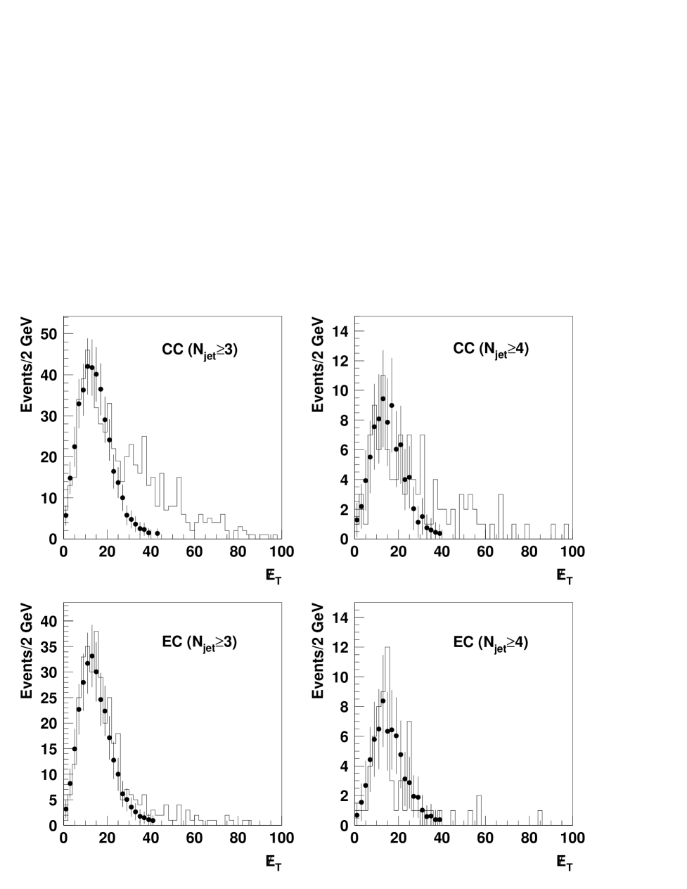
FIG. 4.: ${\hbox{$E$\kern-6.00006pt\lower-0.43057pt\hbox{/}}}_{T}$ spectra of sample 2 (points) normalized to sample 1 (histograms) in the region of $0\leq\mbox{\mbox{${\hbox{$E$\kern-6.00006pt\lower-0.43057pt\hbox{/}}}_{T}$}}\leq 14\;{\rm GeV}$. The normalizations are done for the fake electron in the CC and EC, respectively. The errors are statistical only.

B $t\overline{t}$ background

The number of $t\overline{t}$ background events, $N_{t\overline{t}}$, is calculated using fmcø. The $t\overline{t}$ events were generated using pythia [15] for $m_{\rm top}=175\;\rm{GeV}$. A $t\overline{t}$ production cross section of $\sigma=5.9\pm 1.7\;\rm{pb}$, as measured by DØ [22], is used. The results are $\mbox{$N_{t\overline{t}}$}=27.7\pm 8.3$ events and $\mbox{$N_{t\overline{t}}$}=16.8\pm 5.2$ events for inclusive jet multiplicities of 3 and 4 jets, respectively. The errors include uncertainties on the $t\overline{t}$ production cross section, differences in physics generators, trigger and object identification efficiencies, and on the integrated luminosity.

C $WW+$ jets background

fmcø is also used to calculate the $WW+$ jets background. The production cross section at next-to-leading order is taken as $\sigma=10.40\pm 0.23\;\rm{pb}$ [23, 24], assuming no anomalous couplings ($\delta\kappa=\lambda=0$) [25]. The $WW$ events were generated using pythia. There are $7.7\pm 1.2$ and $1.4\pm 0.3$ events expected for inclusive jet multiplicity of 3 and 4 jets, respectively. The errors include uncertainties on the production cross section, trigger and object identification efficiencies, differences in physics generators, the jet energy scale, and on the integrated luminosity.

D $W+$ jets background

To good approximation, each extra jet in $W+$ jets events is the result of an extra coupling of strength $\alpha_{s}$ [17], and we expect the number of $W+$ jets events to scale as a power of $N_{\rm jet}$. The scaling law is supported by the $W+$ jets, $Z+$ jets, and $\gamma+$ jets data [26]. In this analysis, we first estimate the number of $W+\geq 3$-jet events, $N^{W}_{3}$, in the data collected with ELE_JET_HIGH and ELE_JET_HIGHA triggers, and then extract the effective scaling factor $\alpha$ using $W+\geq n$-jet events collected with EM1_EISTRKCC_MS trigger. The expected number of $W+\geq 4$-jet events ($N^{W}_{4}$) in our base sample is then:

$$N^{W}_{4}=N^{W}_{3}\cdot\alpha\cdot\frac{\varepsilon^{W4}_{\rm trig}}{\varepsilon^{W3}_{\rm trig}},$$ (5)

where $\varepsilon^{W3}_{\rm trig}$ and $\varepsilon^{W4}_{\rm trig}$ are trigger efficiencies of $W+\geq 3$-jet and $W+\geq 4$-jet events, respectively, as shown in Table IV.

1 Estimating the number of $W+\geq n$-jet events

We estimate the number of $W+\geq n$-jet events in a way similar to that used to estimate the multijet background. We first use a neural network (NN) to define a kinematic region in which $W+\geq n$-jet events dominate the background and any possible contribution from mSUGRA can be neglected. In that region, we normalize the number of $W+\geq n$-jet MC events to the number of events observed in the data which have had all other major SM backgrounds subtracted. The normalization factor is then applied to the whole $W+\geq n$-jet MC sample to obtain our estimate for the $W+\geq n$-jet background in the data.

In this analysis, we use a NN package called mlpfit [27]. All NNs have the structure of X-2X-1, where X is the number of input nodes, i.e., the number of variables used for training, and 2X is the number of nodes in the hidden layer. We always use 1 output node with an output range of 0 to 1. Signal events (in this case, $W+\geq n$-jet events) are expected to have NN output near 1 and background events near 0. We choose the NN output region of 0.5–1.0 to be the “signal”-dominant kinematic region. The variables used to distinguish $W+\geq n$-jet events from other SM backgrounds and the mSUGRA signal are:

• ${\hbox{$E$\kern-6.00006pt\lower-0.43057pt\hbox{/}}}_{T}$

• $E^{e}_{T}$

• $H_{T}=\sum E^{j}_{T}$ for all jets with $E^{j}_{T}>15\;{\rm GeV}$

• $\Delta\phi_{e,\mbox{\mbox{${\hbox{$E$\kern-4.20004pt\lower-0.3014pt\hbox{/}}}_{T}$}}}$

• $M_{T}=\sqrt{2E^{e}_{T}\mbox{\mbox{${\hbox{$E$\kern-6.00006pt\lower-0.43057pt\hbox{/}}}_{T}$}}[1-\cos(\Delta\phi_{e,\mbox{\mbox{${\hbox{$E$\kern-4.20004pt\lower-0.3014pt\hbox{/}}}_{T}$}}})]}$

• $\Delta\phi_{j_{1},\mbox{\mbox{${\hbox{$E$\kern-4.20004pt\lower-0.3014pt\hbox{/}}}_{T}$}}}$ (not used for $\geq 4$-jet events)

• $\Delta\phi_{j_{2},\mbox{\mbox{${\hbox{$E$\kern-4.20004pt\lower-0.3014pt\hbox{/}}}_{T}$}}}$ (used for $\geq 2$-jet and $\geq 3$-jet events)

• $\mathcal{A}$—aplanarity [28] (used for $\geq 2$, $\geq 3$, and $\geq 4$-jet events) is defined in terms of the normalized momentum tensor of the $W$ boson and the jets with $E^{j}_{T}>15\;\rm{GeV}$:

  $$M_{ab}=\frac{\sum_{i}p_{ia}p_{ib}}{\sum_{i}p^{2}_{i}},$$ (6)

  where $\vec{p_{i}}$ is the three-momentum of object $i$ in the laboratory frame, and $a$ and $b$ run over the $x$, $y$, and $z$ coordinates. Denoting $Q_{1}$, $Q_{2}$, and $Q_{3}$ as the three eigenvalues of $M_{ab}$ in ascending order, $\mathcal{A}$ $=1.5\times Q_{1}$. The $p_{z}$ of the $W$ boson is calculated by imposing the requirement that the invariant mass of the electron and the neutrino (assumed to be the source of ${\hbox{$E$\kern-6.00006pt\lower-0.43057pt\hbox{/}}}_{T}$) equals the $W$ boson mass. This requirement results in a quadratic equation for the longitudinal momentum of the neutrino. Because the probability of a small $p_{z}$ is usually higher than that of a large $p_{z}$, the smaller $p_{z}$ solution is always chosen. In cases where there is no real solution, ${\hbox{$E$\kern-6.00006pt\lower-0.43057pt\hbox{/}}}_{T}$ is increased until a real solution is obtained.

• $r_{H}=H_{T2}/H_{Z}$, where $H_{T2}=H_{T}-E^{j_{1}}_{T}$, and $H_{Z}=\sum_{i}|p_{z}|$ where $i$ runs over the electron, all jets with $E^{j}_{T}>15\;{\rm GeV}$, and neutrino (as assumed in the calculation of $\mathcal{A}$) in the event [29] (only used for $\geq 4$-jet events).

• $\cos\theta^{*}_{e}$, where $\theta^{*}_{e}$ is the polar angle of the electron in the $W$ boson rest frame, relative to the direction of flight of the $W$ boson. The $W$ boson four-momentum is obtained by fitting the event to a $t\overline{t}$ assumption. The details of the fit are described in Ref. [29] (only used for $\geq 4$-jet events).

• $\cos{\theta}^{*}_{eb}$, where $\theta^{*}_{eb}$ is the angle between the electron and the $b$ jet from the same top (or antitop) quark in the $W$ boson rest frame [30]. Again, a fit to the $t\overline{t}$ assumption is performed to identify the correct $b$ jet (only used for $\geq 4$-jet events).

All the offline requirements described in Sec. III B 4 are applied except that the requirement on the number of jets is reduced corresponding to different inclusive jet multiplicity. The multijet, $t\overline{t}$, and $WW$ backgrounds are estimated using the methods described in Sec. V A–V D. The mSUGRA events were generated with $m_{0}=170\;{\rm GeV}$, $m_{1/2}=58\;{\rm GeV}$ and $\tan\beta=3$. This parameter set was chosen because it is close to the search limit obtained in the dilepton analysis.

2 Estimating $N^{W}_{3}$

The result of the NN training for $\geq 3$-jet events is shown in Fig. 5(a). The number of $W+\geq 3$-jet events used in the training is the same as the sum of all background events, including any possible mSUGRA sources in their expected proportions. The match between training and data is shown in Fig. 5(b), where the data and MC are normalized to each other for NN output between 0.5 and 1.0. Because the number of mSUGRA events is negligible in this region, we do not include them in the background subtraction. We estimate that $241.8\pm 18.0$ $W+\geq 3$-jet events pass our final 3-jet selection.

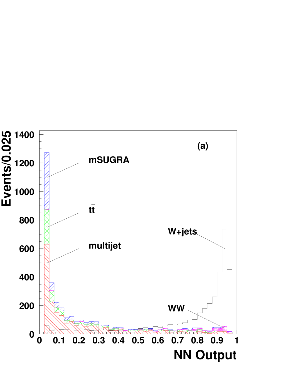
FIG. 5.: (a) Expected NN output for events passing the ELE_JET_HIGH or ELE_JET_HIGHA triggers and with $\geq 3$ jets. (b) Expected NN output for data (points) and the observed NN output for data (histogram). The error on the points include statistical and systematic errors. All events were required to pass our offline selections, except that we required only 3 jets instead of 4.

3 Measuring the scaling factor $\alpha$

We extract the parameter $\alpha$ from the data passing the EM1_EISTRKCC_MS trigger, which does not have a jet requirement in the trigger, and fit the measured number of $W+n$-jet events ($\overline{N}^{W}_{n}$) to:

$$\overline{N}^{W}_{n}=\overline{N}^{W}_{1}\cdot\alpha^{n-1}.$$ (7)

$\overline{N}^{W}_{n}$ values are obtained as described in Sec. V D 1. The NN training and normalization to the data are performed separately for each inclusive jet multiplicity. The results are summarized in Table V. The errors on $\overline{N}^{W}_{n}$ include statistical errors from MC and data, and uncertainties on the choice of different normalization regions and on the choice of different QCD dynamic scales used in generating vecbos events.

The fit of $\overline{N}^{W}_{n}$ to Eq. 7 is shown in Fig. 6, from which we extract $\alpha=0.172\pm 0.007$.

TABLE V.: Estimated number of $W+\geq n$-jet events, $\overline{N}^{W}_{n}$, as a function of inclusive jet multiplicity in the data passing the EM1_EISTRKCC_MS trigger. They were obtained by normalizing MC to data in the NN output region where $W+\geq n$-jets events dominate (see text). $\overline{N}_{\rm data}$ is the number of observed events. The mSUGRA events were generated with $m_{0}=170\;{\rm GeV}$, $m_{1/2}=58\;{\rm GeV}$, and $\tan\beta=3$.

$N_{\rm jet}$	$\geq 1$	$\geq 2$	$\geq 3$	$\geq 4$
$\overline{N}_{\rm data}$	$8191$	$1691$	$353$	$64$
$N_{\rm multijet}$	$826\pm 95$	$291\pm 48$	$75\pm 15$	$16.6\pm 7.0$
$N_{t\overline{t}}$	$25.8\pm 7.6$	$26.1\pm 7.6$	$21.9\pm 6.5$	$13.5\pm 4.3$
$N_{WW}$	$33.7\pm 3.3$	$23.6\pm 2.3$	$6.19\pm 0.95$	$1.12\pm 0.25$
$\overline{N}^{W}_{n}$	$7210\pm 131$	$1283\pm 79$	$230\pm 27$	$27.4\pm 7.4$
$N_{\rm mSUGRA}$	$28.3\pm 3.7$	$25.0\pm 3.1$	$19.7\pm 2.7$	$12.6\pm 2.1$

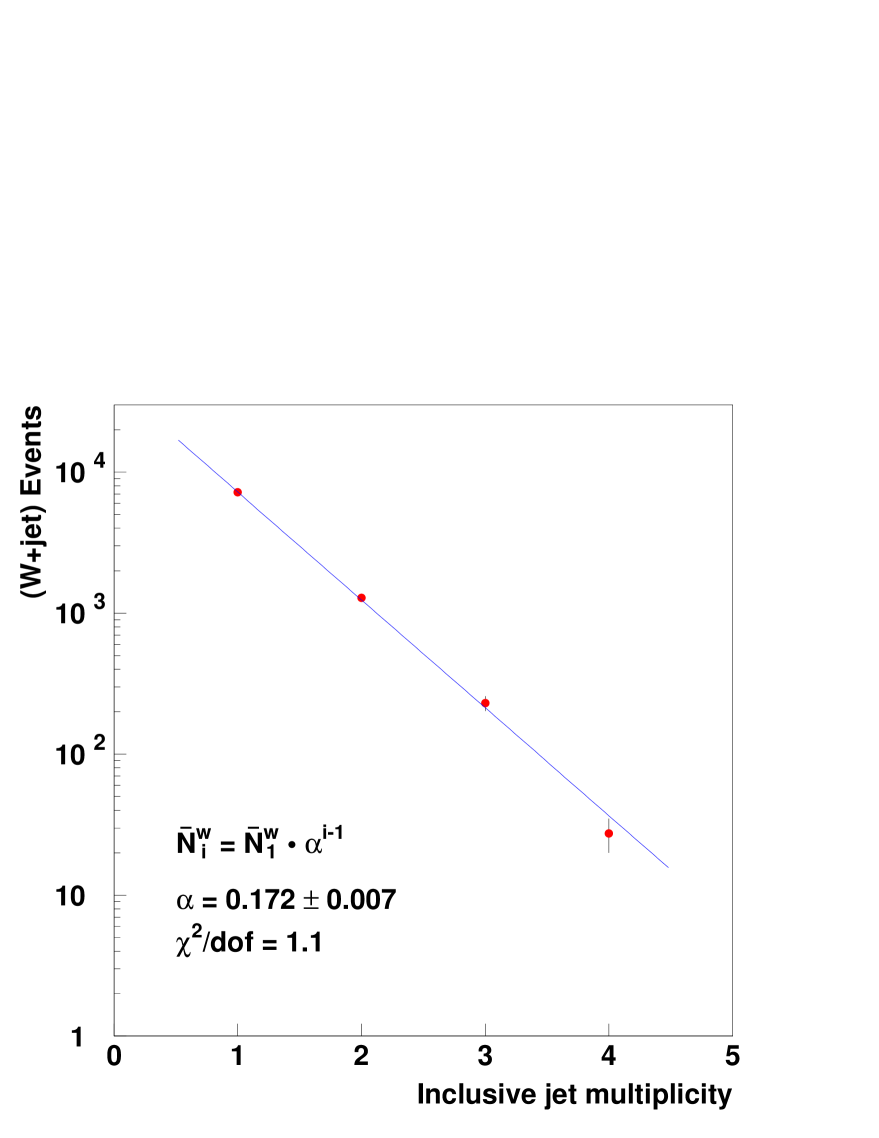
FIG. 6.: Fit of $W+\geq n$-jet events to the power law of Eq. 7.

4 Calculating the number of $W+\geq 4$-jet events, $N^{W}_{4}$

With $\varepsilon^{W3}_{\rm trig}=0.925\pm 0.016$ and $\varepsilon^{W4}_{\rm trig}=0.957\pm 0.012$, and using Eq. 5, we obtain $N^{W}_{4}=43.0\pm 7.6$.

E Summary

The expected numbers of events in the base data sample from the major sources of background are summarized in Table VI. From the table, we conclude that the sum of the backgrounds is consistent with the observed number of candidate events.

TABLE VI.: Expected numbers of events in the base data sample from the major sources of background and the number of observed data events.

$W+\geq 4$-jets	$43.0$ $\pm$ $7.6$
misidentified multijet	$19.1$ $\pm$ $4.7$
$t\overline{t}$	$16.8$ $\pm$ $5.2$
$WW+\geq 2$-jets	$1.4$ $\pm$ $0.3$
Total	$80.3$ $\pm$ $10.4$
Data	72

VI SEARCH FOR SIGNAL

A Neural Network Analysis

We use a NN analysis to define a kinematic region in which the sensitivity of signal to background is highest. We use the following variables in the NN. Those not defined below have been defined in Sec.V D 1.

• ${\hbox{$E$\kern-6.00006pt\lower-0.43057pt\hbox{/}}}_{T}$ – For the signal, ${\hbox{$E$\kern-6.00006pt\lower-0.43057pt\hbox{/}}}_{T}$ comes from two LSPs and at least one neutrino. For the $t\overline{t}$, $W+$ jets, and $WW$ backgrounds, it comes from the neutrino. For multijet background, it comes from fluctuation in the measurement of the jet energy. Generally, the signal has larger ${\hbox{$E$\kern-6.00006pt\lower-0.43057pt\hbox{/}}}_{T}$ than the backgrounds.

• $E^{e}_{T}$ – The electron in the signal comes from a virtual $W$ boson decay. Its spectrum is softer than that of the electrons from the $t\overline{t}$ and $W+$ jets backgrounds.

• $H_{T}$ – A pair of heavy mSUGRA particles are produced in the hard scattering and most of the transverse energy is carried away by jets. The $H_{T}$ for the signal thus tends to be larger than that for the major backgrounds.

• $E^{j_{3}}_{T}$ – The third leading jet in $E_{T}$ from $W+$ jets, $WW$, and multijet events most likely originates from gluon emission. For $t\overline{t}$ and mSUGRA events, it is probably due to $W$ boson decay. Thus, the $t\overline{t}$ and mSUGRA signals have a harder $E^{j_{3}}_{T}$ spectrum.

• $M_{T}$ – For $t\overline{t}$, $W+$ jet, and $WW$ events, $M_{T}$ peaks near $M_{W}=80\;\rm{GeV}$. This is not the case for the signal since we expect the $W$ boson produced in the decay chain to be virtual for a wide range of $m_{1/2}$ up to 200 GeV.

• $\Delta\phi_{e,\mbox{\mbox{${\hbox{$E$\kern-4.20004pt\lower-0.3014pt\hbox{/}}}_{T}$}}}$ – Because the electron and neutrino form a $W$ boson in $t\overline{t}$, $W+$ jet, and $WW$ events, their $\Delta\phi_{e,\mbox{\mbox{${\hbox{$E$\kern-4.20004pt\lower-0.3014pt\hbox{/}}}_{T}$}}}$ spectra should peak away from $\Delta\phi_{e,\mbox{\mbox{${\hbox{$E$\kern-4.20004pt\lower-0.3014pt\hbox{/}}}_{T}$}}}=0$. For multijet events, the $\Delta\phi_{e,\mbox{\mbox{${\hbox{$E$\kern-4.20004pt\lower-0.3014pt\hbox{/}}}_{T}$}}}$ spectrum should peak near 0 and $\pi$ because ${\hbox{$E$\kern-6.00006pt\lower-0.43057pt\hbox{/}}}_{T}$ can be caused by fluctuations in the energy of the jet which mimics an electron.

• $\mathcal{A}$ – $W+$ jets, $WW$, and multijet events are more likely to be collinear due to QCD bremsstrahlung, while the signal and $t\overline{t}$ events are more likely to be spherical.

• $\cos\theta^{*}_{j}$, where $\theta^{*}_{j}$ is the polar angle of the higher-energy jet from $W$ boson decay in the rest frame of parent $W$ boson, relative to the direction of flight of the $W$ boson. This is calculated by fitting all the events to the $t\overline{t}$ assumption. For $t\overline{t}$ production, the spectrum is isotropic, but for the signal and other SM backgrounds, it is not.

• $\cos\theta^{*}_{e}$, the signal has a somewhat different $\cos\theta^{*}_{e}$ distribution than the background does, especially for $t\overline{t}$ events.

The spectra for these variables are shown in Fig. 7. There is no evidence of an excess in our data for the mSUGRA parameters used. Fig. 8 displays the $\cos\theta^{*}_{j}$ and $\cos\theta^{*}_{e}$ distributions for signal and $t\overline{t}$ events. These two variables are particularly useful in reducing the $t\overline{t}$ background relative to the mSUGRA signal. Nevertheless, $t\overline{t}$ events still make the largest contribution in the signal-rich region because of their similarity to the mSUGRA signal. This can be seen in Fig. 9, in which the NN output is displayed for each background and the mSUGRA signal for a particular set of parameters. The result of the NN output for data is given in Fig. 10. The expected background describes the data well.

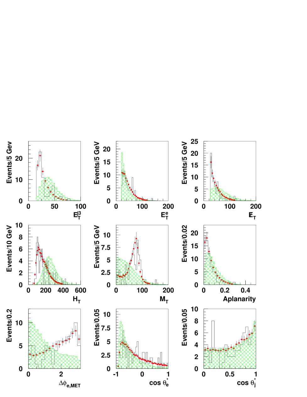
FIG. 7.: Distribution of NN variables for data (open histogram), background (points) and signal (hatched histogram). The signal was generated at $m_{0}=170\;\rm{GeV}$, $m_{1/2}=58\;\rm{GeV}$, and $\tan\beta=3$. We have multiplied the expected number of signal events (18.5) by a factor of 4.3 to normalize it to the total number of background events. Since the same number of signal and background events are used to train the NN, the plot shows the relative strength of signal to background as seen by the NN.

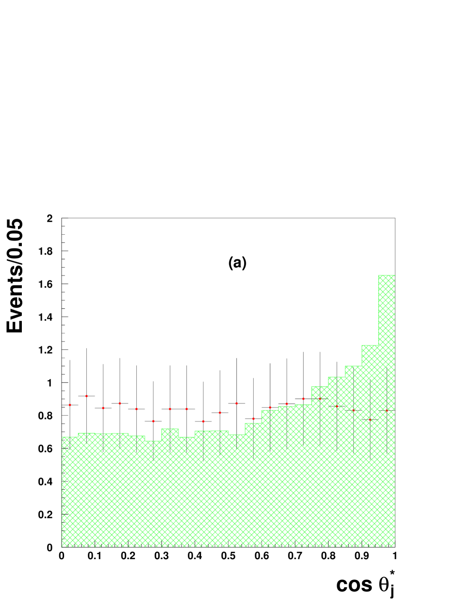
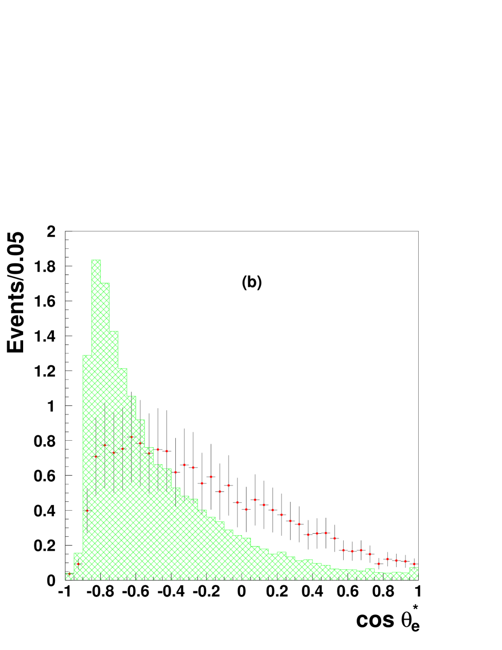
FIG. 8.: Distribution of (a) $\cos\theta^{*}_{j}$ and (b) $\cos\theta^{*}_{e}$ for signal (hatched histogram) and $t\overline{t}$ events (points). The signal was generated at $m_{0}=170\;\rm{GeV}$, $m_{1/2}=58\;\rm{GeV}$, and $\tan\beta=3$. We have multiplied the expected number of signal events (18.5) by a factor of 0.91 to normalize it to the number of $t\overline{t}$ events expected in our base sample.

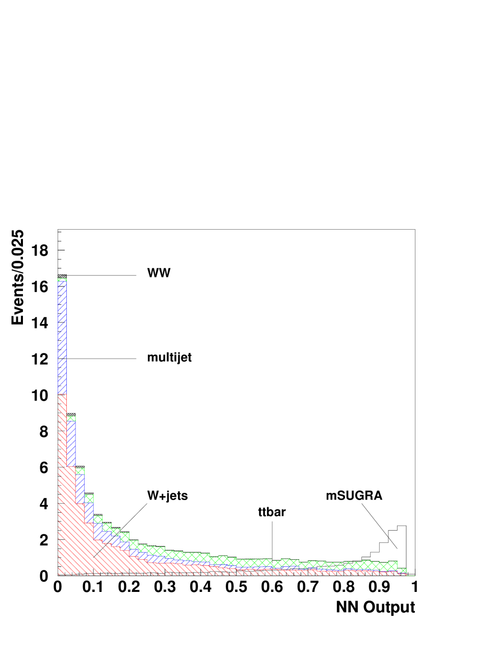
FIG. 9.: Result of training of a NN. The excess above the background near 1 is the expected signal. The signal was generated at $m_{0}=170\;\rm{GeV}$, $m_{1/2}=58\;\rm{GeV}$, and $\tan\beta=3$. The backgrounds are stacked up in the order of $W(e\nu)+$ jets, $W(\tau\nu)+$ jets, misidentified multijet, $t\overline{t}$, and $WW$ production. The contribution of each type of background is normalized to its expected number of events in the data.

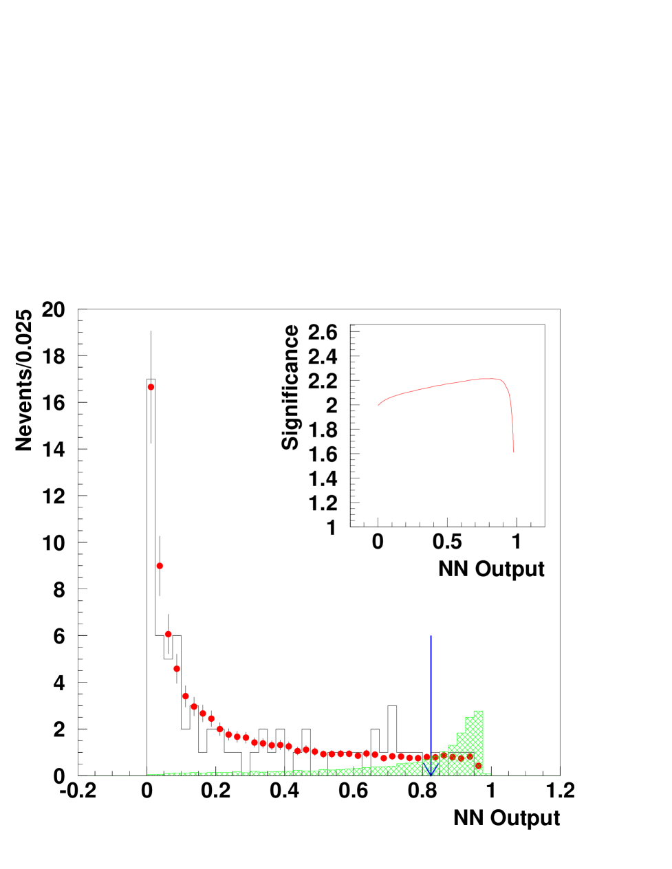
FIG. 10.: NN output for data (open histogram), signal (hatched histogram), and background (points). The signal was generated at $m_{0}=170\;\rm{GeV}$, $m_{1/2}=58\;\rm{GeV}$, and $\tan\beta=3$. The background expectation describes the data well. The vertical arrow indicates the cutoff on the NN output that corresponds to the maximum signal significance. The significance (described in Sec. VI B) as a function of NN output is plotted in the insert.

B Signal Significance

To apply the optimal cut on the NN output, we calculated the signal significance based on the expected number of signal ($s$) and background ($b$) events that would survive any NN cutoff. We define the significance ($\overline{{\mathcal{S}}}$) below. The probability that the number of background events, $b$, fluctuates to $n$ or more events is:

$$F(n|b)=\sum_{k=n}^{\infty}p(k|b)=\frac{1}{\sqrt{2\pi}}\int_{{\mathcal{S}}(n|b)}^{\infty}e^{-t^{2}/2}\ dt,$$ (8)

where $p(k|b)=\frac{b^{k}e^{-b}}{k!}$ is the Poisson probability for observing $k$ events with $b$ events expected. ${\mathcal{S}}(n|b)$ can be regarded as the number of standard deviations required for $b$ to fluctuate to $n$, and it can be calculated numerically. For $s+b$ expected events, the number of observed events can be any number between $[0,\infty)$. The significance is thus defined as:

$$\overline{{\mathcal{S}}}=\sum_{n=0}^{\infty}p(n|s+b)\cdot{\mathcal{S}}(n|b)$$ (9)

where $p(n|s+b)$ is the Poisson probability for observing $n$ events with $s+b$ events expected.

The NN output corresponding to the maximum significance determines our cutoff to calculate the 95% C.L. limit on the cross section. The error on the expected signal includes uncertainties on trigger and object identification efficiencies, on parton distribution functions (10%), differences between MCs (12%), and on the jet energy scale (5%). Table VII lists the results in terms of 95% C.L. limits on production cross sections for various sets of model parameters of mSUGRA.

TABLE VII.: Number of observed events ($N_{\rm obs}$), expected total background events ($N^{\rm total}_{\rm bkgd}$), and expected signal events ($N_{\rm mSUGRA}$), corresponding to the optimal NN cutoff for different sets of mSUGRA parameters. The signal acceptance after NN cutoff (Acceptance), mSUGRA production cross section for each parameter set ($\sigma_{\rm mSUGRA}$), and the calculated 95% C.L. upper limit on the production cross section ($\sigma_{95\%}$) are also listed. All limits are for $\tan\beta=3$.

$m_{0}$	$m_{1/2}$	$N_{\rm obs}$	$N^{\rm total}_{\rm bkgd}$	$N_{\rm mSUGRA}$	${\rm Acceptance}$	$\sigma_{\rm mSUGRA}$	$\sigma_{95\%}$
$(\rm{GeV})$	$(\rm{GeV})$				(%)	$(\rm{pb})$	$(\rm{pb})$
$160$	$60$	$8$	$6.45\pm 1.22$	$11.11\pm 1.97$	$0.360\pm 0.064$	$33.34$	$29.61$
$160$	$65$	$7$	$5.94\pm 1.15$	$7.93\pm 1.41$	$0.364\pm 0.065$	$23.48$	$26.87$
$170$	$58$	$4$	$4.43\pm 0.88$	$10.36\pm 1.83$	$0.301\pm 0.053$	$37.16$	$23.59$
$170$	$65$	$3$	$2.87\pm 0.61$	$5.84\pm 1.03$	$0.283\pm 0.050$	$22.23$	$23.71$
$180$	$60$	$5$	$4.18\pm 0.85$	$8.49\pm 1.50$	$0.305\pm 0.054$	$30.00$	$27.76$
$180$	$67$	$3$	$3.45\pm 0.72$	$5.31\pm 0.94$	$0.306\pm 0.054$	$18.69$	$20.89$
$190$	$55$	$5$	$5.51\pm 1.12$	$11.12\pm 1.97$	$0.248\pm 0.044$	$48.46$	$30.88$
$190$	$63$	$4$	$3.65\pm 0.79$	$6.41\pm 1.13$	$0.299\pm 0.053$	$23.17$	$25.15$
$200$	$57$	$3$	$2.72\pm 0.60$	$6.98\pm 1.23$	$0.208\pm 0.037$	$36.21$	$32.79$
$200$	$62$	$2$	$2.31\pm 0.51$	$5.12\pm 0.91$	$0.231\pm 0.041$	$23.96$	$24.85$
$210$	$53$	$2$	$2.75\pm 0.59$	$6.85\pm 1.21$	$0.096\pm 0.017$	$77.38$	$57.99$
$210$	$60$	$4$	$3.74\pm 0.81$	$5.95\pm 1.05$	$0.238\pm 0.042$	$26.96$	$31.33$
$220$	$50$	$2$	$3.72\pm 0.79$	$7.05\pm 1.25$	$0.054\pm 0.009$	$141.83$	$97.55$
$220$	$55$	$5$	$4.02\pm 0.83$	$7.06\pm 1.25$	$0.169\pm 0.030$	$45.00$	$50.87$
$230$	$45$	$2$	$2.90\pm 0.62$	$5.93\pm 1.05$	$0.030\pm 0.005$	$214.95$	$183.99$
$230$	$50$	$4$	$3.45\pm 0.74$	$5.91\pm 1.04$	$0.046\pm 0.008$	$138.52$	$166.06$
$240$	$43$	$1$	$2.53\pm 0.56$	$5.24\pm 0.93$	$0.023\pm 0.004$	$244.29$	$194.22$
$240$	$52$	$3$	$3.83\pm 0.80$	$5.24\pm 0.93$	$0.056\pm 0.010$	$100.14$	$110.68$
$250$	$41$	$2$	$3.47\pm 0.72$	$5.38\pm 0.95$	$0.021\pm 0.004$	$281.53$	$256.82$
$250$	$42$	$4$	$4.97\pm 0.96$	$5.80\pm 1.03$	$0.024\pm 0.004$	$259.36$	$282.43$
$260$	$41$	$7$	$5.91\pm 1.16$	$5.63\pm 1.00$	$0.022\pm 0.004$	$280.15$	$452.28$
$260$	$42$	$4$	$3.87\pm 0.77$	$4.70\pm 0.83$	$0.020\pm 0.003$	$257.67$	$374.37$

VII RESULTS

We conduct an independent NN analysis on each generated mSUGRA point. The production cross section calculated by pythia is compared with that obtained by limit calculation at 95% C.L. to determine whether the mSUGRA point is excluded or not. Using the two cross sections at each point, we linearly extrapolate between the excluded and non-excluded points to determine the exact location of the exclusion contour. The exclusion contour at the 95% C.L. is plotted in Fig. 11. Shown in the same figure are the results of the DØ dilepton and LEP I [31] analyses.

Our single-electron analysis is particularly sensitive in the moderate $m_{0}$ region. The extended region of exclusion relative to the DØ dilepton result is in the range of $165\;{\rm GeV}<m_{0}<250\;{\rm GeV}$. The dominant SUSY process changes from $\widetilde{g}$$\widetilde{q}$ production at $m_{0}=170\;{\rm GeV}$ to $\widetilde{g}$ pair production at $m_{0}=250\;{\rm GeV}$. The limit worsens as $m_{0}$ increases because the mass difference between $\widetilde{\chi}_{1}^{\pm}$ ($\widetilde{\chi}_{2}^{0}$) and $\widetilde{\chi}_{1}^{0}$ decreases, resulting in softer electron and jets spectra, and consequently reduced acceptance.

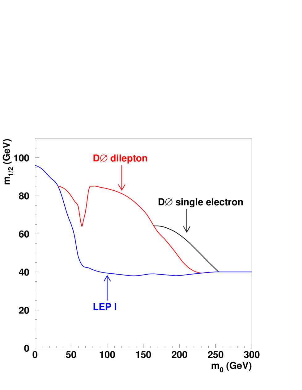
FIG. 11.: Exclusion contour at the 95% C.L. for mSUGRA with $\tan\beta=3$. The result from the DØ dilepton and LEP I analyses are also shown.

As this work was being completed, a related result [32] on searches for mSUGRA in the jets plus missing energy channel at Tevatron appeared. Since its limits on mSUGRA parameters, although more restrictive than those obtained in this work and in the earlier DØ publication [33] in the analogous channel, are expressed in a different parameter plane ($m_{\widetilde{q}}$ vs. $m_{\widetilde{g}}$), we do not show them in Fig. 11.

VIII CONCLUSION

We observe 72 candidate events for an mSUGRA signal in the final state containing one electron, four or more jets, and large ${\hbox{$E$\kern-6.00006pt\lower-0.43057pt\hbox{/}}}_{T}$ in $92.7\;\rm{pb}^{-1}$ data. We expect $80.3\pm 10.4$ such events from misidentified multijet, $t\overline{t}$, $W+$ jets, and $WW$ production. We conclude that there is no evidence for the existence of mSUGRA. We use neural network to select a kinematic region where signal to background significance is the largest. The upper limit on the cross section extends the previously DØ obtained exclusion region of mSUGRA parameter space.

REFERENCES

- [1] Also at University of Zurich, Zurich, Switzerland.
- [2] Also at Institute of Nuclear Physics, Krakow, Poland.
- [3] C. Quigg, “Gauge Theories of the Strong, Weak, and Electromagnetic Interactions,” Addison-Wesley, Reading, MA, 1983, p. 188-189.
- [4] R. Cahn, Rev. Mod. Phys. 68, 951 (1996).
- [5] J. L. Hewett, hep-ph/9810316 (unpublished).
- [6] For a review, see e.g., H. Haber and G. Kane, Phys. Rept. 117, 75 (1985).
- [7] G. R. Farrar and P. Fayet, Phys. Lett. B 76, 575 (1978).
- [8] V. Barger et al., hep-ph/0003154 (unpublished).
- [9] DØ Collaboration, B. Abbott et al., Phys. Rev. D Rapid Comm. 63, 091102 (2001).
- [10] DØ Collaboration, B. Abbott et al., Phys. Rev. Lett. 83, 4937 (1999).
- [11] DØ Collaboration, S. Abachi et al., Nucl. Instr. Methods Phys. Res. A 338, 185 (1994).
- [12] At DØ, we define and to be the polar and azimuthal angles of the physical objects, respectively. We define the pseudorapidity . We denote as the pseudorapidity calculated relative to the center of the detector rather than relative to the reconstructed interaction vertex.
- [13] DØ Collaboration, S. Abachi et al., Phys. Rev. D 52, 4877 (1995).
-
[14]
J. Zhou, Ph.D. thesis, Iowa State University,
2001 (unpublished).
http://www-d0.fnal.gov/results/publications_talks/thesis/johnzhou/thesis.ps. - [15] M. Bengtsson and T. Sjöstrand, Comp. Phys. Comm. 43, 367 (1987); S. Mrenna, Comp. Phys. Comm. 101, 23 (1997); and T. Sjöstrand, L. Lonnblad, and S. Mrenna, hep-ph/0108264 (unpublished).
- [16] G. Marchesini et al., Comp. Phys. Comm. 67, 465 (1992). We used v5.9.
- [17] W. Beenakker, F. A. Berends, and T. Sack, Nucl. Phys. B 367, 32 (1991).
- [18] DØ Collaboration, S. Abachi et al., Phys. Rev. Lett. 79, 1197 (1997).
-
[19]
R. Genik, Ph.D. thesis, Michigan State
University, 1998 (unpublished).
http://www-d0.fnal.gov/results/publications_talks/thesis/genik/thesis_lite.ps. - [20] CERN Program Library Long Writeup W5013, 1994.
- [21] J. Yu, Ph.D. thesis, State University of New York, Stony Brook, 1993 (unpublished). http://www-d0.fnal.gov/results/publications_talks/thesis/yu/jae_thesis_final.ps.
- [22] DØ Collaboration, B. Abbott et al., Phys. Rev. D 60, 012001 (1999).
- [23] J. Ohnemus, Phys. Rev. D 44, 1402 (1991).
- [24] DØ Collaboration, B. Abbott et al., Phys. Rev. D Rapid Comm. 63 031101 (2001).
- [25] K. Hagiwara et al., Nucl. Phys. B 282, 253 (1987).
- [26] DØ Collaboration, S. Abachi et al., Phys. Rev. Lett. 79, 1203 (1997).
-
[27]
J. Schwindling and B. Mansoulié, “MLPFIT”,
http://schwind.home.cern.ch/schwind/MLPfit.html (unpublished). - [28] V. Barger and R. Phillips, “Collider Physics,” Addison-Wesley, Reading, MA, 1987, p. 281.
- [29] DØ Collaboration, B. Abbott et al., Phys. Rev. D 58, 052001 (1998).
- [30] G. Mahlon and S. Parke, Phys. Lett. B 411, 173 (1997).
- [31] LEPSUSYWG, ALEPH, DELPHI, L3, and OPAL experiments, http://www.cern.ch/LEPSUSY.
- [32] CDF Collaboration, T. Affolder et al., Phys. Rev. Lett. 88, 041801 (2002).
- [33] DØ Collaboration, B. Abbott et al., Phys. Rev. Lett. 83, 4937 (1999).