SEARCH FOR A HIGGS BOSON

DECAYING TO MASSIVE VECTOR BOSON PAIRS

AT LEP

Jeremiah M. Mans

A DISSERTATION
PRESENTED TO THE FACULTY
OF PRINCETON UNIVERSITY
IN CANDIDACY FOR THE DEGREE
OF DOCTOR OF PHILOSOPHY

RECOMMENDED FOR ACCEPTANCE
BY THE DEPARTMENT OF
PHYSICS

June 2002

$\copyright$ Copyright by Jeremiah Mans, 2002. All rights reserved.

Abstract

In the Standard Model, the Higgs boson is responsible for mass-generation and stabilizing the electroweak interaction at high energies. The boson has not been observed and the Standard Model does not predict its mass. Direct searches have excluded the existence of a Higgs boson with a mass less than 113 GeV. Searches to date have focussed on b-quark decays of the Higgs, but the model predicts an increased branching fraction to massive vector boson pairs for a heavier Higgs. In some extensions of the Standard Model which predict multiple Higgs bosons, the lightest Higgs boson couples primarily to bosons, not fermions. Results excluding these “fermiophobic” models have used the two-photon decay to date, but for Higgs masses above 100 GeV, the decay to massive vector boson pairs dominates. In this dissertation, I present the first search for a Higgs boson decaying to massive vector boson pairs. The search is based on data collected by the L3 experiment at CERN during the 1999-2000 period.

The search uses the Higgsstrahlung production mode where the Higgs is radiated from an off-shell Z boson, so the analysis must include the decay of the Z boson as well as the decay of the two W or Z bosons from the Higgs decay. The events will contain six final state fermions, and the decays of the W and Z define nine different channels for the $\textrm{h}\rightarrow\textrm{WW}$ search. I present the details and results of analyses for six of the channels. The combined analyses exclude a fermiophobic Higgs decaying to massive vector boson pairs for $83.8\textrm{ GeV }<m_{\scriptsize\mathrm{h}}<104.2\textrm{ GeV}$ at a 95% confidence level with an unexcluded region between $88.8\textrm{ GeV}<m_{\scriptsize\mathrm{h}}<89.6\textrm{ GeV}$. Monte Carlo predictions of the analyses’ performance predict an exclusion range of $86.8\textrm{ GeV }<m_{\scriptsize\mathrm{h}}<107.5\textrm{ GeV}$. I also present model-independent branching ratio limits for the massive vector boson search, as well as a scan of the fermiophobic plane combining with the results of the LEP $\textrm{h}\rightarrow\gamma\gamma$ search.

Chapter 1 LEP and the L3 Experiment

The machine does not isolate man from the great problems of nature
but plunges him more deeply into them.

Antoine de Saint-Exupéry

1.1 LEP

LEP is the “Large Electron-Positron” storage ring built 40 meters under the countryside outside Geneva, Switzerland. The epithet “large” was well chosen, since LEP is the largest accelerator in the world at 27 km in circumference. Construction of the accelerator began in 1982 and the first collisions in the detectors were recorded on August 13,1989[1]. There are four large general-purpose detectors equally spaced around the ring: L3, Aleph, Delphi, and Opal. The locations of the four detectors are indicated in Figure 1.1.

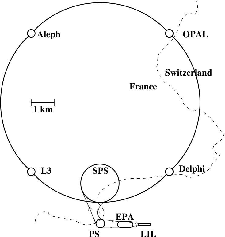
Figure 1.1: Overhead sketch of LEP and the rest of the CERN accelerator complex.

LEP sits at the end of a long chain of accelerators which work together to accelerate electrons and positrons up to kinetic energies of 100 GeV and above. The electron and positron bunches are produced in the Linear Injector for LEP (LIL) complex and stored at 600 MeV in the Electron-Positron Accumulator (EPA). From the EPA, the bunches are transfered to the CERN Proton Synchrotron (PS), where the magnets are ramped down to accept the low-energy bunches. The PS accelerates the bunches to 2.5 GeV and transfers them on to the Super Proton Synchrotron (SPS) which provides the last pre-acceleration kick up to 22 GeV for transfer into LEP. The LEP machine then accelerates the bunches up to full energy, brings the beams into collision, and keeps them in collision for several hours until the stored current drops to the point where the operators decide to dump the beam.

Up until 1996, LEP ran at or near the Z pole ($\sqrt{s}=91.2\textrm{ GeV}$). In 1996, CERN began adding superconducting cavities to LEP, which allowed the beam energy to increase each year. At the beginning and end of each year, a few $\textrm{pb}^{-1}$ of data was taken at the Z pole for calibration. Most of the data was taken at energies near the upper limit of the machine. This limit increased as additional accelerating cavities were added and the physicists and engineers of the machine group tuned the machine for ever higher gradients and beam energies. Between 1998 and 1999, CERN upgraded the cryogenic systems as part of preparations for the LHC. The upgrade allowed the machine group to push the accelerating gradient of the superconducting cavities from their design of 6MV/m to more than 7.5MV/m. During the 1999 run, the beam energy was limited for several weeks by statute: the original permit granted by the French nuclear authorities had specified beam energies up to, but not exceeding 100 GeV, which limited $\sqrt{s}$ to 200 GeV. Once the authorities amended the permit, the experiments collected a month’s worth of data at 202 GeV, and LEP even reached 204 GeV for one 15 minute run. The breakdown of luminosity versus $\sqrt{s}$ over the 1999-2000 running period is given in Table 1.1.

	$\sqrt{s}$ ($\pm 1\textrm{ GeV}$)	Luminosity ($\textrm{pb}^{-1})$
1999	191.6	29.8
	195.5	83.7
	199.5	82.8
	201.8	37.0
2000	203.1	9.6
	205.0	68.9
	206.5	130.3
	208.0	8.5

Table 1.1: Luminosity collected by the L3 experiment over 1999-2000.

In 2000, the machine operation was optimized for discoveries in the Higgs and supersymmetric sectors, which required the maximum possible beam energies. The machine group developed several improvements to LEP operations which significantly improved the energy reach and integrated luminosity collected in 2000 [2].

• The upgraded cryogenics system increased the stability of the RF system, which allowed the operations group to reduce the margin from two klystrons to one. At full beam energy, the LEP RF system suffered a klystron trip due to overheating about once an hour. With a one-klystron margin, the RF system could absorb one trip, but a second occurring before the first klystron could be restarted caused beam loss. The reduced margin allowed an increase in $\sqrt{s}$ of 1.5 GeV.

• The machine group reduced the 350 MHz RF frequency driving the cavities by 100 Hz to expand the orbit of the beams. The larger orbit reduced the synchrotron radiation and allowed the dipolar component of the quadrupole magnets to control the new orbit. The reduced frequency also increased the RF margin slightly by reshaping the bunches. These adjustments allowed an increase in $\sqrt{s}$ of 1.4 GeV.

• The machine group also enabled unused corrector magnets as additional dipoles to further increase the effective LEP radius, which added another 400 MeV.

• Eight old LEP1 copper cavities were reinstalled, adding an additional 30MV in total accelerating gradient. This gradient increase translated to an increase in $\sqrt{s}$ of $\sim 400\textrm{ MeV}$. The increase in energy is larger than the gradient increase because LEP does not have to accelerate the beams from rest each turn, but rather just replace the energy lost to synchrotron radiation.

• The machine’s mode of operation was modified to add “miniramps.” In previous years, once the machine reached its target energy and the beams entered collision, the energy did not change. In 2000, the operators would raise the energy several times during the physics coast as the RF stabilized and current fell. Thus, a given fill would generate data at several $\sqrt{s}$ values.

The beam loss rate sharply increased with LEP operating at its limit. Of the roughly 4000 fills made in the twelve years of LEP running, 1400 were made in the last year. To reduce the impact to physics beam time, the machine group made special efforts to reduce the turnaround time. The group was able to reduce the average turnaround time from beam dump to stable collisions to less than an hour from the previous average of about 2 hours. In the search for maximum energy, some of the accelerating cavities were stressed beyond their limits and the machine group had to reduce the maximum gradient of several during the year. Some of these cavities recovered, but others did not. The continual changes to the machine operating conditions meant that the 2000 dataset contained data from many different $\sqrt{s}$ energies, as shown in Figure 1.2. For analysis purposes, we grouped the data into the four energy bins indicated in the plot.

Figure 1.2: Distribution of luminosity as a function of $\sqrt{s}$ in 2000.

The four energy bins used for the $\textrm{h}\rightarrow\textrm{WW}/\textrm{ZZ}$ search are indicated by the dashed lines.

1.2 The L3 Experiment

The L3 experiment, located at point 2 on the LEP ring, is shown in perspective view in Figure 1.3[3].

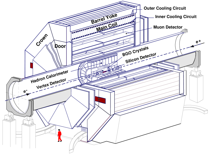
Figure 1.3: Perspective view of the L3 experiment.

The entire L3 experiment, the largest of the four LEP detectors, is surrounded by a 7800 ton octagonal conventional solenoid electromagnet which produces a 0.5 T field. Within the electromagnet are the muon detection chambers, the calorimeters, and, closest to the beam pipe, the inner tracking subdetectors. All of the detector elements are mounted on a 281-ton steel support tube suspended along the central axis of the detector. The muon chambers are mounted on the outside of the support tube and the rest of the subdetectors are inside. While the LEP machine experienced many changes in beam elements and operating procedures during 1998-2000, the L3 experiment was extremely stable. No major subdetectors were added during this time, and the calibration procedures for the detector were perfected.

1.2.1 The Inner Tracking Subdetectors

The L3 experiment contains two major tracking subdetectors. The role of these detectors is to measure the paths of charged particles through the magnetic field with a minimum of disturbance to the particles’ paths and energies. The curvature of these tracks reveals the charge and momentum of the particles. Very close to the beampipe there are two layers of silicon strip detectors which are called the Silicon Microvertex Detector (SMD). Around the SMD is a gas-filled drift chamber called the Time-Expansion Chamber (TEC).

The TEC consists of a long cylindrical tube filled with a mixture of 80% $\textrm{CO}_{2}$ and 20% isobutane $\left(\textrm{iC}_{4}\textrm{H}_{10}\right)$. Charged particles passing through the tube ionize the gas molecules. The TEC collects and times the arrival of the gas ions to determine the path of the charged particles. The chamber is divided into two rings – an inner ring of 12 sectors and an outer ring of 24 sectors. These sectors are defined by the arrangement of wires strung parallel to the beam pipe. Most of the wires carry high voltages which supply the drift and amplification electric fields, while the rest carry the collected charge out to high speed analog-to-digital converters.

Figure 1.4: The drift and amplification fields of the TEC.

Charged particles ionize the gas, which drifts in a relatively low field toward the grid wires. After passing the grid, the ions are accelerated in a higher field and produce secondary ions which are also collected at the anode.

The fields set up in a TEC sector are shown in schematic view in Figure 1.4. Each track is measured by up to 51 sense wires to determine $r-\phi$ accurately. Additional charge-division wires provide some information about the $z$ position of the track. There are also two cathode strip chambers mounted on the outside of the TEC which measure the $z$ position of the track with average 300 $\mu\textrm{m}$ resolution. The analyses in this thesis use the TEC, along with the SMD, for measuring tracks in jets and identifying the isolated groups of odd-numbered tracks associated with taus.

In 1991, the radius of the LEP beampipe was reduced from 8 cm to 5.5 cm, which opened enough space to add a new silicon tracking detector, the SMD [4]. The SMD is a silicon strip detector, composed of silicon wafers with metalized strips on both sides of the wafer. The wafers are made of n-type silicon and have p-type strips implanted on one side with a 25 $\mu\textrm{m}$ pitch to measure $r-\phi$. On the opposite side are $\textrm{n}^{+}$-type strips with a wider readout pitch of 150 $\mu\textrm{m}$ to 200 $\mu\textrm{m}$ that measure $r-z$. Charged particles passing through the silicon wafer produce electron-hole pairs that drift to a collection strip and the collected charge is read out. The SMD improved the tracking resolution of the detector significantly. The SMD is particularly important for reconstructing the primary vertex (where the initial electron and position interaction occurred within the beampipe) as well as for determining the location of secondary vertices such as those from decays of B mesons. A schematic $r-\phi$ view of the SMD along with some tracks which might be expected from Z boson pair production are shown in Figure 1.5.

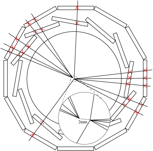
Figure 1.5: $r-\phi$ view of the Silicon Microvertex Detector.

The figure shows hits in the SMD and the tracks which might be expected from a $\textrm{ZZ}\rightarrow\textrm{e}^{+}\textrm{e}^{-}\textrm{b}\bar{\textrm{b}}$ event. One of the B mesons has traveled 2mm in $r-\phi$ before decaying at a displaced vertex.

1.2.2 Calorimetry

In contrast to tracking, where the goal is to measure position and momentum with very little disturbance of the particle, the goal in calorimetry is to absorb the particle’s energy completely and measure it. Because of the differing interaction lengths of electrons/photons versus pion/other hadrons, two types of high energy calorimeters are required: electromagnetic calorimeters for electrons and photons and hadron calorimeters for pions, kaons, and other hadrons. L3 has very good calorimeters for both electromagnetic and hadronic showers. The electromagnetic calorimeter(BGO) is a crystal calorimeter built out of Bismuth Germanate, $\textrm{Bi}_{4}(\textrm{GeO}_{4})_{3}$, and the hadron calorimeter (HCAL) is built out of uranium plates with interspersed proportional chambers.

The BGO electromagnetic calorimeter is a very important feature of the L3 detector. The calorimeter is formed from 11,000 individual 2 cm $\times$ 2 cm $\times$ 24 cm crystals which point at the interaction region. The heavy, high-charge nuclei in BGO cause a strong electromagnetic cascade and eventually convert a fraction of the electrons’ and photons’ energy into scintillation light, which is measured using a photodiode. Crystal calorimeters did not originate with the L3 detector, but L3 was the first large-scale detector to use BGO as the crystal material. The BGO has an average energy resolution of $\frac{\sigma_{E}}{E}=\frac{1.57\%}{\sqrt{E}}+0.34\%$ for electrons. The shower profile in the crystals surrounding the peak crystal is also useful for separating hadrons, including $\pi_{0}$’s, from electrons and photons. The very high resolution of the calorimeter is important for measuring the electrons from Z decays and accurately determining recoil masses.

As L3 was originally constructed, there was a small gap between the barrel section of the BGO and the endcap. During the 1995-1996 shutdown, a new subdetector was installed to fill the gap – the so-called EGAP detector[5]. The detector is constructed of lead blocks with scintillating fibers embedded longitudinally. Electromagnetic showers in the lead generate light in the fibers. The light from the fibers is coupled into plastic lightguides which are read out by phototriodes. There are 24 blocks on each end of the BGO barrel to provide coverage of the region $38^{\circ}<\theta<42^{\circ}$ and $138^{\circ}<\theta<142^{\circ}$. The EGAP detector has poorer resolution than the BGO, at $12\%/\sqrt{E}$, but the difference is relatively unimportant for searches: the increased hermeticity of the detector is of greater importance.

The L3 HCAL, like most hadron calorimeters, is a sampling calorimeter. The L3 HCAL consists of a series of depleted uranium plates interspersed with gas proportional chambers. Most of the nuclear interactions occur in the uranium and the gas chambers sample the developing shower.

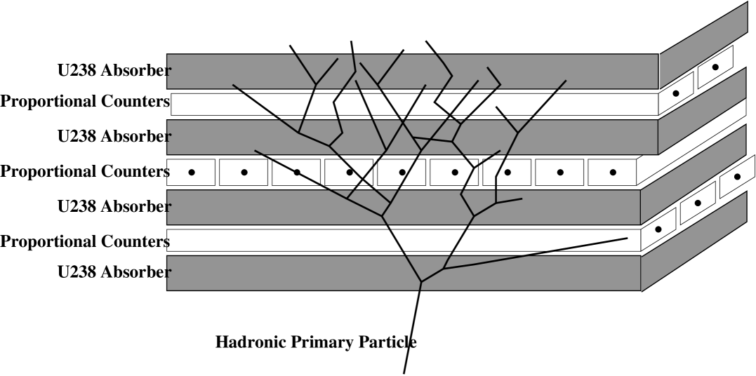
Figure 1.6: Schematic view of the HCAL showing shower development.

A schematic view of a shower developing in a portion of the HCAL is shown in Figure 1.6. In the central barrel region, there are 58 uranium layers in each module, while modules in the more forward region have 51 layers. The HCAL is used in the analyses described in this thesis to measure the energies of hadronic jets from Z and W decays.

The L3 calorimeters work together to measure leptons and jets which may be produced in any direction within the detector. The performance of the calorimetry systems can be seen particularly well in Figure 1.7. This figure shows the jet energy measured by the calorimeter for Z-peak jets as a function of the angle of the jet. The two jets produced from Z decay on the peak should sum to $\approx 91$ GeV, as seen in the figure. The sum and resolution are nearly constant for all jet production angles, despite the different barrel, endcap, and EGAP calorimeters which are used to compute the jet energies.

Figure 1.7: Distribution of jet-energy as a function of the cosine of the thrust angle.

This plot shows the sum of jet energies from Z-pole data. The resolution is quite uniform across the entire detector, including the EGAP ($0.74<\cos\theta<0.81$)[6].

1.2.3 Muon Chambers

Besides the BGO electromagnetic calorimeter, the L3 muon chambers are the most unique feature of the detector. They are unique not in their construction or design but rather in their location. They are located inside the magnet and flux-return yoke instead of outside as is more common. This location provides the most uniform bending field and reduces the multiple scattering of the muons on their way out of the detector. Muons are the only particle, besides of course the neutrinos, which emerge from the inner layers of BGO and uranium with most of their energy intact. Thus they are the only particles left to be measured by these tracking chambers. The muon system consists of three layers of drift chambers spaced 145 cm apart, with each layer forming an octagon centered on the interaction point. The chambers are actively aligned using an LED-lens-quadrant photodiode system and the alignment can be verified by ultraviolet laser shots that simulate infinite-momentum muons produced at the interaction point. Each chamber measures the position of passage of a muon with an average accuracy of 168 $\mu\textrm{m}$, which is sufficient to provide a 2% error measurement of muon momentum for 50 GeV muons.

The main muon chambers provide detector coverage in the barrel region between $44^{\circ}$ and $136^{\circ}$. In 1995, an additional set of chambers was added on the flux-return doors of the main solenoid to provide measurements down to within $24^{\circ}$ of the beam line [7]. These forward-backward muon chambers use a 1.24T toroidal field in the iron door to bend forward muons in the region between the chambers. The coils to generate the toroidal field were added as part of the detector upgrade, as well as resistive plate chambers for triggering on forward muons.

Despite the depth of the experiment underground, cosmic ray muons do penetrate down to L3. With very precise arrival-time information about these muons, it is possible to reject those which do not occur in time with a beam crossing. Since the muon chambers cannot provide this information, there is a layer of scintillator panels located between the BGO and the HCAL. These scintillation panels are read out by high speed photomultipliers and time-to-digital converters. The scintillator system has a timing resolution of about 1 ns, which allows the separation of cosmic ray muons from muon pairs produced at the interaction point. A cosmic ray muon would require 5.8 ns to travel across from top scintillator panel to bottom scintillator panel, while a di-muon pair would arrive on the two sides simultaneously.

1.2.4 Monte Carlo

There are very few background-free event signatures for a Higgs produced at LEP, so it is important to understand the behavior of the detector for various Standard Model processes known to be present as well as for the predicted process. For processes which are well-understood theoretically, example events can be generated by sampling the theoretical distributions in a random manner. This technique is called Monte Carlo (MC) and is widely used in high energy physics and in many other fields.

A primary process such as $\textrm{e}^{+}\textrm{e}^{-}\rightarrow\textrm{WW}\rightarrow\textrm{c}\bar{\textrm{s}}\mu\nu$ is specified by the user, and MC generator creates events of this process using a level of accuracy defined by the number of Feynman diagrams included in the generator. The generator carries out the processes of hadronization and quark decay. The generator produces a list of four-vectors representing the “stable” mesons, baryons, photons, and leptons produced in the event. L3 uses several different MC generator programs depending on the processes which are under study. Table 1.2 lists several of the important generators and what processes are generated using them for the work presented in this thesis.

Of course, the detector does not produce a list of four-vectors; it reports energies in calorimeter cells and hits in trackers. In order to match the Monte Carlo with the data, the list of four-vectors must be converted to the same form as data from the detector. This difficult task is carried out by a simulation program based on GEANT 3.15[8]. This program simulates the response of the entire detector to this event. The simulation includes the full complex geometry of the detector, with material-specific properties for both the active regions and for structural elements that may cause scattering or shower initiation. The interaction of hadrons inside the detector is handled by a package called GEISHA[9]. The result of the simulation is stored in the same format as that used for the data, and from this point the same reconstruction and analysis techniques can be applied identically to data and Monte Carlo.

Generator	Processes
PYTHIA[10]	$\begin{array}[]{c}\textrm{e}^{+}\textrm{e}^{-}\rightarrow\textrm{ZZ}\\ \textrm{e}^{+}\textrm{e}^{-}\rightarrow\textrm{Ze}^{+}\textrm{e}^{-}\\ \textrm{e}^{+}\textrm{e}^{-}\rightarrow\textrm{ZH}\end{array}$
KK2F[11]	$\begin{array}[]{l}\textrm{e}^{+}\textrm{e}^{-}\rightarrow\textrm{q}\bar{\textrm{q}}(\gamma)\\ \textrm{e}^{+}\textrm{e}^{-}\rightarrow\mu^{+}\mu^{-}(\gamma)\\ \textrm{e}^{+}\textrm{e}^{-}\rightarrow\tau^{+}\tau^{-}(\gamma)\end{array}$
KORALW[12]	$\textrm{e}^{+}\textrm{e}^{-}\rightarrow\textrm{WW}$
EXCALIBUR[13]	$\begin{array}[]{l}\textrm{e}^{+}\textrm{e}^{-}\rightarrow\textrm{q}\bar{\textrm{q}}^{\prime}\textrm{e}\nu\\ \textrm{e}^{+}\textrm{e}^{-}\rightarrow\textrm{f}_{1}\bar{\textrm{f}}^{\prime}_{1}\textrm{f}_{2}\bar{\textrm{f}}^{\prime}_{2}\end{array}$
PHOJET[14]	$\textrm{e}^{+}\textrm{e}^{-}\rightarrow\textrm{e}^{+}\textrm{e}^{-}\textrm{q}\bar{\textrm{q}}$

Table 1.2: Partial list of Monte Carlo Generators used by L3.

Generation, production, and reconstruction of Monte Carlo is a complicated and CPU-intensive process which is managed from CERN, but carried out at multiple institutes around the world. Farms of PCs are used as well as idle workstations around the experiment during evenings and weekends.

Chapter 2 Theory of the Higgs Boson

[In a system of physics] we adopt, at least insofar as we are reasonable, the simplest conceptual scheme into which the disordered fragments of raw experience can be fitted and arranged.

Willard Van Orman Quine

2.1 Review of the Standard Model

The Standard Model (SM) of particle physics, developed by Weinberg, Glashow, and Salam [15, 16, 17], has proven to be an extremely effective theory for predicting the results of high-energy physics experiments over the last 25 years. The model was developed in the 1960s and 1970s to bring together the results of many different experiments and ad hoc theories. The theory describes the behavior of three forces: the electromagnetic force which acts between charges, the weak force which is responsible for beta decay, and the strong force felt only by quarks and which binds the nuclei of atoms. The theory is silent about gravity, which is too weak at these scales to be felt. The forces are carried by gauge bosons: the $\textrm{W}^{+}$,$\textrm{ W}^{-}$, and Z of the weak interaction, the photon ($\gamma$) of the electromagnetic interaction, and the gluons of the strong interaction. The matter constituents of the theory are twelve particles that are organized into three generations of quarks and three generations of leptons and neutrino partners. The two lightest quarks, the up and down quarks, combine to form protons and neutrons in normal matter, while the lightest charged lepton is the familiar electron. All the particles of the Standard Model are listed in Table 2.1. The discoveries of the gluon in 1979[18] and the W and Z particles in 1983[19, 20] were major triumphs for the Standard Model.

$\left(\begin{array}[]{cc}\mbox{\huge u}&\begin{array}[]{c}+2/3\\ 1-5\end{array}\\ \mbox{\huge d}&\begin{array}[]{c}-1/3\\ 3-9\end{array}\end{array}\right)$	$\left(\begin{array}[]{cc}\mbox{\huge c}&\begin{array}[]{c}+2/3\\ 1150-1350\end{array}\\ \mbox{\huge s}&\begin{array}[]{c}-1/3\\ 75-170\end{array}\end{array}\right)$	$\left(\begin{array}[]{cc}\mbox{\huge t}&\begin{array}[]{c}+2/3\\ 174300\end{array}\\ \mbox{\huge b}&\begin{array}[]{c}-1/3\\ 4000-4400\end{array}\end{array}\right)$
$\left(\begin{array}[]{cc}\mbox{\huge$\nu_{\textrm{e}}$}&\begin{array}[]{c}0\\ 1-5\end{array}\\ \mbox{\huge e}&\begin{array}[]{c}-1\\ 0.51\end{array}\end{array}\right)$	$\left(\begin{array}[]{cc}\mbox{\huge$\nu_{\mu}$}&\begin{array}[]{c}0\\ <0.2\end{array}\\ \mbox{\huge$\mu$}&\begin{array}[]{c}-1\\ 106\end{array}\end{array}\right)$	$\left(\begin{array}[]{cc}\mbox{\huge$\nu_{\tau}$}&\begin{array}[]{c}0\\ <18\end{array}\\ \mbox{\huge$\tau$}&\begin{array}[]{c}-1\\ 1777\end{array}\end{array}\right)$
Fermions
Bosons
$\gamma$$\begin{array}[]{c}0\\ 0\end{array}$	g$\begin{array}[]{c}0\\ 0\end{array}$	H$\begin{array}[]{c}0\\ ?\end{array}$
$\textrm{W}^{\pm}$$\begin{array}[]{c}\pm 1\\ 80419\end{array}$	Z$\begin{array}[]{c}0\\ 91118\end{array}$

Table 2.1: Constituent particles of the Standard Model.

Each particle is listed with its charge and the particle’s mass in MeV as listed in the Particle Data Book [21]. For reference, recall that the mass of the proton is 938 MeV. The d,s, and b quarks and the charged leptons are collectively referred to as “down-type” particles, while u,c,t, and the neutrinos are “up-type”.

The Standard Model is a quantum field theory, where all particles appear as fields and their behavior and interaction can be described by a Lagrangian. For example, a massless fermion field $\psi$ freely propagating through space has a Lagrangian of the form

$${\cal L}=i\,\hbar c\,\bar{\psi}\,\gamma^{\mu}\,\partial_{\mu}\,\psi$$

while a massless vector (spin-1) boson field $A^{\mu}$ has a free Lagrangian of the form

$${\cal L}=-\frac{1}{16\pi}(\partial^{\mu}A^{\nu}-\partial^{\nu}A^{\mu})(\partial_{\mu}A_{\nu}-\partial_{\nu}A_{\mu})=-\frac{1}{16\pi}F^{\mu\nu}F_{\mu\nu}.$$

Interactions between bosons and fermions are written as terms like

$${\cal L}_{\textrm{int}}=-(q\,\bar{\psi}\,\gamma^{\mu}\,\psi)A_{\mu},$$

involving three fields. There are also terms which describe the interaction of four boson fields. The full Standard Model Lagrangian is quite large, but all of the terms have one of these basic forms. In the case of the photon and Z, the two fermions involved are the same flavor, while the W couples to a weak isospin doublet such as $\mu$ and $\nu_{\mu}$ or charm and strange quarks.

2.2 Motivation for a Higgs

In the above discussion of fields, the bosons were explicitly massless, but the physical W and Z are indeed quite massive. The simplest way to add a boson mass term to the Lagrangian is to append

$$m^{2}B_{\mu}B^{\mu}.$$

However, this term is not invariant under transformations which take $B_{\mu}\rightarrow B_{\mu}-\partial_{\mu}\chi$. Therefore, some other gauge-invariant technique is needed to provide masses. Gauge-invariance is a very important principle in quantum field theories because it guarantees a theory to be renormalizable [22]. Renormalization is a process of canceling the many infinities which can appear in the field theory allowing reasonable calculations to be performed.

The gauge-invariant solution used in the Standard Model is the Higgs mechanism. To understand the SM’s Higgs mechanism, consider first the simpler situation of a theory which contains only a massless gauge boson $A^{\mu}$ to which we add a massless complex scalar field $\phi$ [23]. For this situation, the Lagrangian has the form

$${\cal L}=(D_{\mu}\phi)^{*}(D^{\mu}\phi)+\mu^{2}\phi^{*}\phi-\lambda(\phi^{*}\phi)^{2}-\frac{1}{4}F^{\mu\nu}F_{\mu\nu},$$

with the covariant derivative $D^{\mu}=\partial^{\mu}+igA^{\mu}$ to achieve invariance under a local gauge transformation. We see that the scalar field has its minimum at $\phi=\sqrt{\mu^{2}/2\lambda}=v/\sqrt{2}$. If we expand the field near the minimum as $\phi=\left(v+h(x)\right)/\sqrt{2}$ we obtain

$${\cal L} = \frac{1}{2}\left[(\partial_{\mu}-igA_{\mu})(v+h)(\partial^{\mu}+igA^{\mu})(v+h)\right]$$

$$+\frac{1}{2}\mu^{2}(v+h)^{2}-\frac{1}{4}\lambda(v+h)^{4}-\frac{1}{4}F^{\mu\nu}F_{\mu\nu}.$$

This Lagrangian contains the term $\frac{g^{2}v^{2}}{2}A_{\mu}A^{\mu}$, which is a mass term for the (previously massless) gauge boson, obtained in a gauge-invariant manner. The term $\lambda v^{2}h^{2}$ is a mass term for the quantum excitation of the scalar field – a new massive scalar boson. In addition, there are $hAA$, $h^{3}$, and $h^{4}$ interaction terms. The mass of the $A$ boson fixes $v^{2}$ but $\lambda$ is not predicted by the model, and the mass of the scalar is a free parameter.

In review, the algebra above converted an apparently massless complex scalar field with two degrees of freedom into a real massive field and the longitudinal polarization state of the gauge boson, again two total degrees of freedom. The SM, with $\textrm{W}^{+}$, $\textrm{W}^{-}$, and Z to provide mass for, must have at least an SU(2) doublet of complex scalar fields, $\phi=\left(\begin{array}[]{c}\phi^{+}\\ \phi^{0}\end{array}\right)$. Symmetry-breaking is initiated by giving a vacuum expectation only to the real part of the neutral field $\left\langle\phi^{0}\right\rangle=v/\sqrt{2}$. Three of the degrees of freedom become the longitudinal polarizations of the massive weak bosons, and the fourth remains as a real observable scalar boson, the Higgs boson.

With the Higgs mechanism it is also possible to add masses for the fermions in the theory using Yukawa-type terms. Since the left-handed fermions in the SM are SU(2) doublets and the right-handed fermions are SU(2) singlets, a mass term such as

$$m\bar{f}\,f=m(\bar{f}_{L}f_{R}+\bar{f}_{R}f_{L})$$

is not SU(2) invariant. With the Higgs SU(2) doublet, we may write an interaction Lagrangian

$${L}_{{\scriptsize\textrm{int}}}=g_{f}\left[(\bar{f}_{L}\phi)f_{R}+(\phi^{\dagger}\bar{f}_{R})f_{L}\right],$$

where $g_{f}$ is different for each fermion. This interaction Lagrangian transforms satisfactorily under SU(2), although it is an unusual Lagrangian since it explicitly contains the conjugate of the Higgs field. When the Higgs acquires a vacuum expectation,

$$\phi\rightarrow\left(\begin{array}[]{c}0\\ \frac{v+h}{\sqrt{2}}\end{array}\right),$$

the fermion interaction becomes

$${L}_{{\scriptsize\textrm{int}}}=\frac{g_{f}v}{\sqrt{2}}\bar{f}f+\frac{g_{f}}{\sqrt{2}}\bar{f}fh.$$

The first part of the interaction Lagrangian is a mass term for the fermion, where $m_{f}=\frac{g_{f}v}{\sqrt{2}}$. The values $g_{f}$ are free parameters, so the model does not predict the masses of the fermions. Instead, one measures the mass of the fermion experimentally and uses $m_{f}$ equation as a definition of $g_{f}$, so $g_{f}\equiv\frac{\sqrt{2}m_{f}}{v}$. With this substitution, the second part of the interaction Lagrangian becomes

$$\frac{\sqrt{2}m_{f}}{v}\bar{f}fh.$$

This is an interaction term between the fermion and the Higgs particle, describing the vertex in Figure 2.1 which has a coupling proportional to the mass of the fermion.

Figure 2.1: Higgs-fermion vertex.

2.3 Production of a Higgs Boson

In order to search for the Higgs at an accelerator, the experimental production and decay of the Higgs must be considered. The production mechanism for the Higgs is very dependent on the collider used to produce it. In the case of LEP, only the diagrams beginning with an $\mathrm{e^{+}e^{-}}$ pair are relevant. The direct coupling of the Higgs to $\mathrm{e^{+}e^{-}}$ is very small since the coupling is proportional to the fermion mass, which is extremely small for the electron. Therefore, the direct $\mathrm{e^{+}e^{-}}\rightarrow\textrm{H}$ production rate is very small, and indirect processes dominate. There are two classes of indirect production which are important at LEP: Higgsstrahlung and vector boson fusion. In these indirect processes, additional particles are produced along with the Higgs, so their presence and possible decays must be taken into account when describing the physical signature of a Higgs-containing event.

The first type of indirect production is the so-called Higgsstrahlung process, where the electron and positron annihilate to produce an off-shell Z (Z*). The Z* decays to its mass-shell by emitting a Higgs in a manner quite similar to Bremsstrahlung. The Feynman diagram for this process is shown in Figure 2.2a. The physical signature of the event includes the decay products of a Z boson as well as the Higgs. This associated Z can be used to tag the Higgs events. Also, since the Z and Higgs are produced in a two-body decay of the Z* produced at rest, the momentum of the Z should be equal to that of the Higgs; thus the event should be balanced in the detector. For a high rate, the final Z should be near its mass shell, which implies a production mass limit of $m_{{\scriptsize\textrm{H}}}\widetilde{<}\sqrt{s}-m_{\scriptsize\mathrm{Z}}$. Thus, if the Higgs’s mass is less than 116 GeV, LEP should be able to produce it by Higgsstrahlung with a center-of-mass energy of 207 GeV.

(a) Higgsstrahlung	(b) W fusion	(c) Z fusion

Figure 2.2: Production diagrams for the Higgs at LEP.

The second class of diagrams is the vector boson fusion diagrams, both W fusion and Z fusion. In W fusion, the incoming electron and positron emit W bosons which combine to form a Higgs. The emission of the W boson converts the electron and positron into a neutrino and antineutrino respectively, as shown in Figure 2.2b. Z fusion is similar except the scattered electron and positrons remain in the final state (Figure 2.2c). Since fusion diagrams are three-body processes which involve a t-channel diagram, the Higgs produced in the fusion process will have an arbitrary boost relative to the experiment. Also, the missing mass (for W fusion) or $\mathrm{e^{+}e^{-}}$ invariant mass (for Z fusion) will not have any particular value since neither corresponds to any resonance.

The greater cross-section and kinematic advantages of Higgsstrahlung over the fusion diagrams mean that the searches are tuned for the HZ process, despite the resulting search limit at $m_{{\scriptsize\textrm{H}}}=\sqrt{s}-m_{\scriptsize\mathrm{Z}}$. Above that limit, the fusion diagrams dominate, but the absolute rate is too small for an effective search at LEP. As a result, we will consider only HZ production for this thesis, which means we must take into account the decay products of the Z in our analysis.

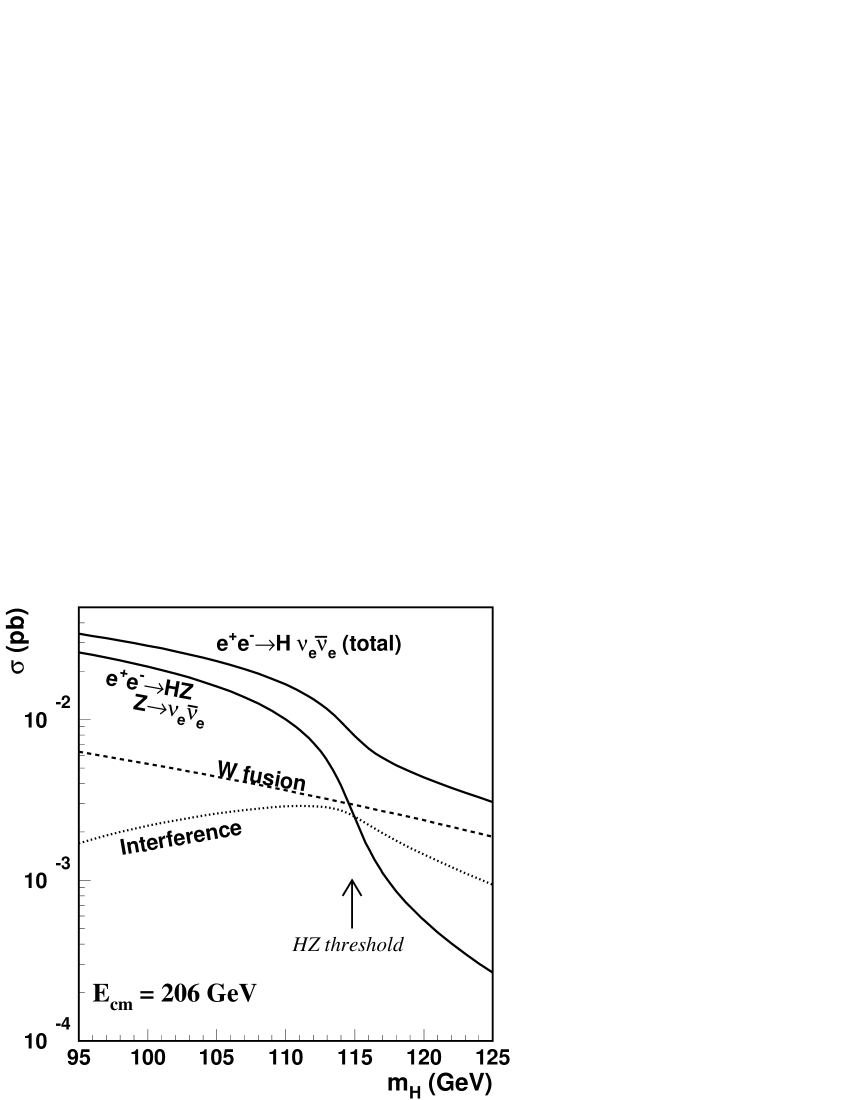
Figure 2.3: Cross-sections for different production diagrams for the process $\mathrm{e^{+}e^{-}}\rightarrow\textrm{H}\nu_{e}\bar{\nu}_{e}$.

The plot is shown for $\sqrt{s}=206\textrm{ GeV}$. For $m_{{\scriptsize\textrm{H}}}<115\textrm{ GeV}$, the Higgsstrahlung process dominates the cross-section. For higher Higgs masses, the W fusion process becomes dominant, but the total cross-section becomes small. There is also an interference term which is important when the two diagrams have similar strength near 115 GeV.

2.4 Decays of the Higgs

The decay of the Higgs is independent of how it is produced, so the same decay channels will occur in the same ratio at any collider. However, the relative usefulness of different decay modes of the Higgs (and associated particles) will vary depending on the background processes at different kinds of colliders. For example, at hadron machines there are many jets arising from soft QCD interactions, so the decays of the Higgs and associated particles into jets would be less useful than those with leptons or photons in the final state. At LEP, the jet-like backgrounds are easier to control through momentum and mass constraints, so the importance of a channel depends more on its branching ratio.

The decay of the Higgs is very dependent on the detailed physics of the Higgs, which implies strong model-dependence. The structure of the electroweak symmetry-breaking puts strong limits on the Z-H-Z vertex, which means that for most models the production rate is similar. The models are primarily distinguished by their decays. In the Standard Model, the expected decays of the Higgs depend on the mass of the Higgs. The general rule is that the Higgs will primarily decay to the heaviest particles kinematically available, since the Higgs coupling is proportional to mass. Thus, for a Higgs with mass between 12 GeV and ~150 GeV, the SM predicts the Higgs will decay primarily to $\textrm{b}\bar{\textrm{b}}$, with small branching fractions into $\tau^{+}\tau^{-}$ and $\textrm{c}\bar{\textrm{c}}$ at lower mass and a rising branching fraction to gauge boson pairs at higher mass. Although the gluon is massless, there is also a substantial Higgs branching fraction to two gluons through top-quark loops. For Higgsstrahlung searches at LEP, $\textrm{b}\bar{\textrm{b}}$ is the most important channel, as seen in Figure 2.4.

Figure 2.4: Predicted branching fractions for a minimal Standard Model Higgs.

The branching fractions are from the standard LHWG database and were calculated using the HZHA program [24].

2.5 Two Higgs Doublet Models

In the minimal SM, after providing longitudinal polarizations to the massive weak bosons there is one degree of freedom left which becomes the Higgs boson. A more general assumption is that there are two doublets of complex scalar fields, $\phi_{1}$ and $\phi_{2}$. Many theorists find advantages in this more extensive Higgs sector. As a group, these models are called “Two-Higgs-Doublet Models” or 2HDMs. The most general 2HDM potential[23] is quite extensive:

$$V = \lambda_{1}(\phi^{\dagger}_{1}\phi_{1}-v_{1}^{2})^{2}+\lambda_{2}(\phi^{\dagger}_{2}\phi_{2}-v_{2}^{2})^{2}$$

$$+\lambda_{3}\left[(\phi^{\dagger}_{1}\phi_{1}-v_{1}^{2})+(\phi^{\dagger}_{2}\phi_{2}-v_{2}^{2})\right]$$

$$+\lambda_{4}\left[(\phi^{\dagger}_{1}\phi_{1})(\phi^{\dagger}_{2}\phi_{2})-(\phi^{\dagger}_{1}\phi_{2})(\phi^{\dagger}_{2}\phi_{1})\right]$$

$$+\lambda_{5}\left[\textrm{Re}(\phi^{\dagger}_{1}\phi_{2})-v_{1}v_{2}\cos\xi\right]^{2}$$

$$+\lambda_{6}\left[\textrm{Im}(\phi^{\dagger}_{1}\phi_{2})-v_{1}v_{2}\sin\xi\right]^{2}.$$

If $\sin\xi\neq 0$, then the theory will break CP explicitly, so we will set $\xi=0$ which makes the potential minimum

$$\left\langle\phi_{1}\right\rangle=\left(\begin{array}[]{c}0\\ v_{1}\end{array}\right),\;\left\langle\phi_{2}\right\rangle=\left(\begin{array}[]{c}0\\ v_{2}\end{array}\right).$$

After significant algebra to remove the Goldstone bosons, we are left with two charged Higgs bosons: $\textrm{H}^{\pm}$, one CP-odd scalar: A⁰, and two CP-even physical scalars: H and h. These last two physical scalars are constructed from a linear combination of the $\phi_{1}$ and $\phi_{2}$ fields as

H $$= \sqrt{2}\left[\left(\Re(\phi^{0}_{1})-v_{1}\right)\cos\alpha+\left(\Re(\phi^{0}_{2})-v_{2}\right)\sin\alpha\right]$$

h $$= \sqrt{2}\left[-\left(\Re(\phi^{0}_{1})-v_{1}\right)\sin\alpha+\left(\Re(\phi^{0}_{2})-v_{2}\right)\cos\alpha\right],$$

where $\alpha$ is the mixing angle between the doublets and the two CP-even scalars. By convention, the h is the less-massive of the two CP-even bosons. The sum $v^{2}_{1}+v^{2}_{2}$ is set by the mass of the W boson, so there are six free parameters: four Higgs boson masses, $\alpha$, and $\tan\beta\equiv v_{2}/v_{1}$.

When one wishes to couple the Higgs fields of the 2HDM model to the particles of the Standard Model, there are several different strategies. In one type of model, one doublet couples to the up-type quarks and leptons and the other to the down-type fermions. This type of model is referred to as a “Type II 2HDM.” The most well-known Type II model is the Minimal Supersymmetric Standard Model (MSSM) [25, 26, 27]. Alternatively, one can construct a model where one doublet couples to bosons and the other to fermions, which is a Type I model. In this type of model, the coupling of the lightest Higgs to fermions is proportional to $\cos\alpha$. Thus, for values of $\alpha\rightarrow\frac{\pi}{2}$, the couplings of the light Higgs to fermions tend toward zero. The model is generally referred to as a “fermiophobic” model, since the light Higgs does not couple to the fermions [28].

Since the fermiophobic Higgs does not couple directly to $\textrm{b}\bar{\textrm{b}}$ or $\tau^{+}\tau^{-}$ as in the Standard Model, what decay channels does this leave? Somewhat surprisingly, a low-mass fermiophobic Higgs decays primarily to two photons. The Higgs does not couple directly to the photon, but it can decay through a W loop or a charged Higgs loop, as shown in the 2.5a. For a low mass fermiophobic Higgs boson, the two photon decay is expected to be dominant, and all the LEP experiments have carried out searches for it. These analyses are reviewed in Chapter 4 before their results are combined with the $\textrm{h}\rightarrow\textrm{WW}/\textrm{ZZ}$ channels to fully cover the fermiophobic search.

(a) Loop diagrams for $\textrm{h}\rightarrow\gamma\gamma$.	(b) Higgs decay to a pair of Z or W bosons.

Figure 2.5: Leading decay diagrams for a fermiophobic Higgs.

The fermiophobic Higgs can also decay to a pair of weak gauge bosons. At the masses which LEP can reach, the Higgs cannot decay to two real W’s or Z’s, so the decay is $\textrm{h}\rightarrow V^{*}V^{*}$, where the star indicates that the vector boson is off its mass shell. How far off mass shell? Consider the differential width for $\textrm{h}\rightarrow\textrm{W}^{(*)}\textrm{W}^{*}\rightarrow\textrm{f}_{1}\bar{\textrm{f}}^{\prime}_{1}\textrm{f}_{2}\bar{\textrm{f}}^{\prime}_{2}$: [29]

$$d\Gamma_{h} = dm^{2}_{(*)}dm^{2}_{*}\frac{g^{6}m_{W}^{2}\sqrt{\lambda(m^{2}_{(*)},m^{2}_{*},m^{2}_{h})}}{16(4\pi)^{8}m_{h}}\cdot$$

$$\left|\frac{{\cal F}_{1}(\theta^{(*)}_{\textrm{f}_{1}},\theta^{*}_{\textrm{f}_{2}})}{(m^{2}_{(*)}-m^{2}_{W}+im_{W}\Gamma_{W})(m^{2}_{*}-m^{2}_{W}+im_{W}\Gamma_{W})}\right|^{2}{\cal F}_{2}(\textrm{f}_{1}){\cal F}_{2}(\textrm{f}_{2}),$$

where $m_{(*)}$ is the mass of the W boson closer to its mass shell, and $m_{*}$ that of the lighter W. The angles $\theta^{(*)}_{\textrm{f}_{1}}$ and $\theta^{*}_{\textrm{f}_{2}}$ are measured in the rest frame of the appropriate W boson. The functions are defined as

$${\cal F}_{1} = 2m_{(*)}m_{*}(1-\cos\theta^{(*)}_{\textrm{f}_{1}}\cos\theta^{*}_{\textrm{f}_{2}})+(m^{2}_{h}-m^{2}_{(*)}-m^{2}_{*})\sin\theta^{(*)}_{\textrm{f}_{1}}\sin\theta^{*}_{\textrm{f}_{2}}$$

$${\cal F}_{2}(\textrm{f}_{\textrm{j}}) = \left\{\begin{array}[]{ll}1&,\textrm{ for leptons}\\ 3\left|V_{\textrm{f}_{\textrm{j}}\bar{\textrm{f}}^{\prime}_{\textrm{j}}}\right|^{2}&,\textrm{ for quarks}\end{array}\right.$$

$$\lambda(a,b,c) = \left(1-\frac{a}{c}-\frac{b}{c}\right)^{2}-\frac{4ab}{c^{2}}.$$

Examining the denominator of the differential width, it is clear that the width is maximized for $m_{(*)}\approx m_{\scriptsize\mathrm{W}}$ and $m_{*}\approx\sqrt{s}-m_{\scriptsize\mathrm{Z}}-m_{\scriptsize\mathrm{W}}$ . This effect can be seen clearly by plotting the invariant masses for the W’s produced by the Pythia MC generator in Figure 2.6. Thus, at LEP fermiophobic Higgs decays should have one vector boson near its mass-shell and the other far off it. This feature strongly influenced the design of analyses intended to search out the Higgs in this channel.

Figure 2.6: Generated mass of W bosons in $\textrm{h}\rightarrow\textrm{WW}$.

This plot shows the masses of the W bosons produced by the PYTHIA Monte Carlo generator with $m_{\textrm{h}}=105\textrm{ GeV}$ and $\sqrt{s}=206$ GeV. The solid curve represents the more massive W produced while the dashed curve which represents the lighter W. The heavier W has an average mass of 71.7 GeV with a pronounced peak at 80 GeV, while the lighter W has an average mass of 22.6 GeV.

The relative rates of the $\textrm{h}\rightarrow\gamma\gamma$ channel and the $\textrm{h}\rightarrow\textrm{WW}/\textrm{ZZ}$ channels within a Higgs model depend on the details of the model. The partial widths of $\textrm{h}\rightarrow\textrm{WW}$ and $\textrm{h}\rightarrow\textrm{ZZ}$ are dominated by direct coupling terms which are strongly constrained by the Higgs’s role in generating the masses of the W and Z bosons. We may thus assume the rates of $\textrm{h}\rightarrow\textrm{ZZ}$ and $\textrm{h}\rightarrow\textrm{WW}$ to be in constant proportion. Conversely, the $\textrm{h}\rightarrow\gamma\gamma$ decay is entirely dependent on loops, which makes it more sensitive to the details of the theory and thus more model-dependent. As a baseline of comparison, the LEP Higgs Working Group settled on a benchmark model which produces the branching ratios plotted in Figure 2.7. All results use these branching ratios unless otherwise stated.

Figure 2.7: Branching fractions of the benchmark fermiophobic model.

2.6 Indirect Measurements of the Higgs Mass

Although the Higgs has not been observed, its presence can potentially be deduced by a careful study of standard electroweak processes. The Standard Model predicts higher-order corrections to many processes which are sensitive to the masses of the bosons and the heavier quarks. For example, the major process studied at LEP for the first five years was $\mathrm{e^{+}e^{-}}\rightarrow f\bar{f}$ via the Z resonance, including $\mathrm{e^{+}e^{-}}\rightarrow\textrm{Z}\rightarrow\textrm{b}\bar{\textrm{b}}$. This process has significant corrections from top quarks, including the diagram in Figure 2.8a. The presence of the top quark in these loop diagrams allowed the LEP Electroweak Working Group to predict $m_{{\scriptsize\textrm{t}}}=173^{+12\>+18}_{-13\>-20}\textrm{ GeV}$ in 1994 [30]. The CDF and D0 collaborations published the first direct observation of the top quark in 1995 with the mass values of $m_{{\scriptsize\textrm{t}}}=176\pm 8(\textrm{stat}.)\pm 10(\textrm{syst}.)\textrm{ GeV}$ [31] and $m_{{\scriptsize\textrm{t}}}=199_{-21}^{+19}(\textrm{stat}.)\pm 22(\textrm{syst}.)\textrm{ GeV}$ [32] respectively. The agreement between the indirect prediction and the observation is quite remarkable.

(a) $\textrm{Z}\rightarrow\textrm{b}\bar{\textrm{b}}$ corrected by a top-containing	(b) $\textrm{Z}\rightarrow f\bar{f}$ corrected by a Higgs loop.
triangle.

Figure 2.8: Example corrections to basic LEP I electroweak diagrams from top and Higgs loops.

The electroweak observables are sensitive to $m_{{\scriptsize\textrm{t}}}$ to order $m^{2}_{{\scriptsize\textrm{t}}}$ , but they are also sensitive to $\log m_{\scriptsize\mathrm{h}}$, which allows indirect limits on $m_{\scriptsize\mathrm{h}}$ to be set with sufficient data. This dependency arises from diagrams such as 2.8b, which is essentially the virtual form of the Higgsstrahlung diagram. The success of the LEP electroweak fits encouraged the combination of the original LEP I results with data from Stanford Linear Detector (SLD), W mass measurements from the Tevatron and LEP II, and even results from neutrino-nucleon scattering and atomic parity violation in Cesium atoms. When the data from all these sources are combined, the electroweak fit establishes a favored region for the Standard Model Higgs. With enough independent data, the electroweak fit becomes a strong test of the internal consistency of the Standard Model.

The most recent results of the electroweak fit for the Higgs mass are given in Figure 2.9 [33].

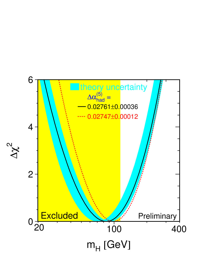
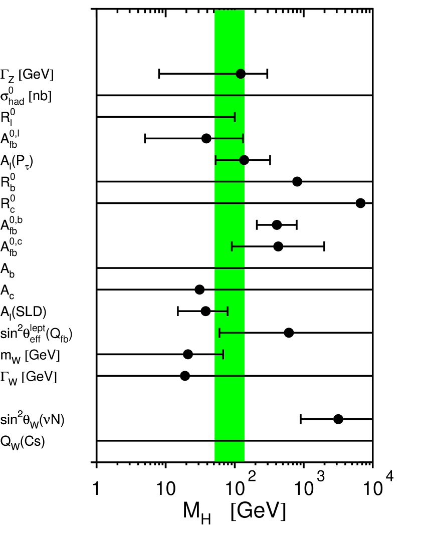
Figure 2.9: Results of the most recent electroweak fit for the Higgs mass.

Several of the results used in this fit are preliminary and the fit itself should also be considered preliminary at this time [33].

Figure 2.9a shows the result of the Standard Model fit for the Higgs combining all the observations. The fit favors a low mass for the Higgs, around 85 or 95 GeV depending on the value of $\Delta\alpha^{(5)}_{{\scriptsize\textrm{had}}}$ chosen. The presence of the Higgs has been excluded by the direct Standard Model search up to $\approx 113$ GeV. The results of the fit suggest that the Higgs might be within the reach of the LEP experimental data.

Figure 2.9b gives the favored Higgs mass region for particular sets of the input data to the fit. Many of the input parameters do not have sufficient sensitivity to the Higgs mass to set useful limits, and several of the sensitive parameters are not in agreement. The left-right asymmetry measured at the SLD and the W mass measurement favor a low Higgs mass (around 40 GeV) while the forward-backward asymmetry measured at LEP and other measurements favor a much heavier Higgs mass above 200 GeV. The overall $\chi^{2}$ of the electroweak fit fairly poor at 29 for 15 degrees of freedom. The electroweak fit indicates that all is not well with the Standard Model and suggests that the problem may be in the Higgs sector. Unfortunately, the electroweak fit is sufficiently complicated that no work has been done to determine if a Type I 2HDM might better fit the electroweak data. A direct search is certainly worthwhile given the indications of the electroweak data.

Chapter 3 The Search Process for $\textrm{h}\rightarrow\textrm{V}^{(*)}\textrm{V}^{*}$

Algebra is a jolly game; we go searching for x, only we don’t know what it is…

Hermann Einstein

Prior to 1999, neither the Standard Model nor the benchmark fermiophobic model predicted any success in a search for a Higgs decaying to massive boson pairs. The maximum energy achieved by the LEP accelerator was 189 GeV, implying a Higgsstrahlung reach to 99 GeV, a mass too low for a significant rate in most models. However, the significant beam energy increases of late 1999 and 2000 extended the search range above 110 GeV : the point in the Standard Model where $\textrm{BR}(\textrm{H}\rightarrow\textrm{W}^{*}\textrm{W}^{*})$ becomes larger than $\textrm{BR}(\textrm{H}\rightarrow\tau^{+}\tau^{-})$, and thus becomes the second-largest decay. At such masses, the decay to massive boson pairs also dominates the benchmark fermiophobic model.

Any Higgs decay to massive boson pairs within the reach of the Higgsstrahlung process at LEP necessarily involved a virtual boson, which incurs a penalty in the rate. The W is lighter than the Z, so it naturally dominates the branching fraction for the LEP mass range. In fact, there is an additional exchange term arising from the distinguishablity of $\textrm{W}^{+}$and $\textrm{W}^{-}$ versus Z and Z, so the $\textrm{h}\rightarrow\textrm{WW}$ is expected to dominate for all Higgs masses. Accordingly, we focused on $\textrm{h}\rightarrow\textrm{WW}$, but supplemented the search with $\textrm{h}\rightarrow\textrm{ZZ}$ where possible.

In the $\textrm{e}^{+}\textrm{e}^{-}\rightarrow\textrm{Zh}\rightarrow\textrm{f}\bar{\textrm{f}}\textrm{W}^{(*)}\textrm{W}^{*}$ search, there are nine different channels, defined by the decays of the Z and the two W bosons. These nine channels are listed in Table 3.1, along with their theoretical branching fractions.

			$\textrm{WW}\rightarrow$
			qqqq	(47%)	qql$\nu$	(43%)	l$\nu$l$\nu$	(10%)
	qq	(70%)	qqqqqq	(32.8%)	qqqql$\nu$	(30.2%)	qq$\textrm{l}\nu\textrm{l}\nu$	(7.0%)
$\textrm{Z}\rightarrow$	$\nu\nu$	(20%)	$\nu\nu\textrm{qqqq}$	(9.4%)	$\nu\nu\textrm{qql}\nu$	(8.7%)	$\nu\nu\textrm{l}\nu\textrm{l}\nu$	(2.0%)
	ll	(10%)	llqqqq	(4.7%)	llqql$\nu$	(4.4%)	lll$\nu$l$\nu$	(1.0%)

Table 3.1: Channels of the $\textrm{h}\rightarrow\textrm{WW}$ search and theoretical branching fractions.

Branching fractions are calculated using the most recent results from the Particle Data Group [21].

We constructed channel names by first listing the decay products of the Z boson and then listing the four decay products from the two W bosons. For example, in the $\textrm{qqqql}\nu$ channel, the Z decays to $\textrm{q}\bar{\textrm{q}}$, one W decays to $\textrm{q}\bar{\textrm{q}}^{\prime}$ and the other W decays to $\textrm{l}\nu$.

The potential search significance of a channel depends on both the expected background level after selection and the intrinsic physical branching fraction of the channel. To estimate the number of expected signal events, assume that all 217 $\textrm{pb}^{-1}$ of 2000 data was taken at $\sqrt{s}=206\textrm{ GeV}$, where the $\textrm{e}^{+}\textrm{e}^{-}\rightarrow\textrm{Zh}$ cross-section for $m_{\scriptsize\mathrm{h}}$=110 GeV is 0.15 pb and the benchmark branching ratio $\textrm{h}\rightarrow\textrm{WW}$ is 86%. The total number of events expected would be 28 events in all channels, assuming 100% efficiency. Applying the branching ratios yields an expectation of less than one event in the $\nu\nu\textrm{l}\nu\textrm{l}\nu$ and $\textrm{lll}\nu\textrm{l}\nu$ channels; these channels are likely to be unimportant for the search. On the other hand, a qqqqqq analysis would provide ~9 events, which could be a significant number depending on the signal-background separation which is possible in the analysis.

Of the nine channels, we have analyzed six of them: qqqqqq, qqqql$\nu$, $\nu\nu$qqqq, $\nu\nu\textrm{qql}\nu$, llqqqq and qql$\nu$l$\nu$. The analyses of each channel follow the same pattern:

1. A set of preselection cuts removed the “obvious” background events. These preselection cuts remove classes of events which appear in the data, but are not well covered by Monte Carlo. These include cosmic muon events, beam-gas events, and some types of two-photon events.

2. More difficult backgrounds were removed at the final selection step using one or more neural networks. All the analyses used a common class of neural network techniques described in Appendix A.2. These networks were trained to produce an output of zero for background events and one for signal events.

3. Final distributions of the selected signal, background, and data were produced, generally using a discriminant combination of the neural networks and a reconstructed Higgs mass as described in Appendix A.3.

How much background needed to be removed? Figure 3.1 is a plot of cross-section measurements made at L3 of different Standard Model processes as a function of center-of-mass energy. Near $\sqrt{s}=91\textrm{ GeV}$, the Z pole is clearly visible in the $\textrm{e}^{+}\textrm{e}^{-}\rightarrow\textrm{q}\bar{\textrm{q}}(\gamma)$ cross-section. At 160 GeV, W pair production crosses threshold, and Z pair production turns on around 183 GeV. Down in the lower right corner is the predicted cross-section for a $m_{\scriptsize\mathrm{h}}=110\textrm{ GeV}$ Higgs. Thus, we attempted to detect a process which is predicted to occur at a rate five orders of magnitude smaller than the many Standard Model background processes, so significant data analysis efforts were required to remove background and isolate any candidate signal events.

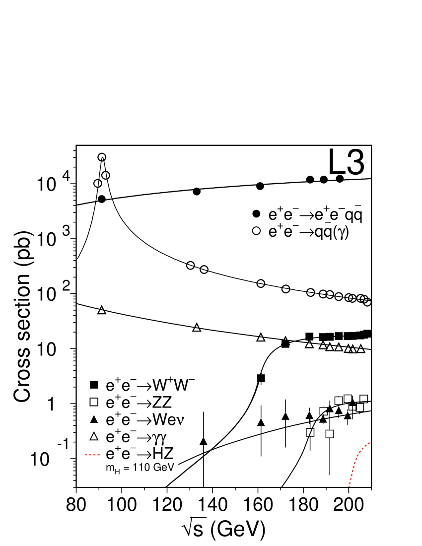
Figure 3.1: Cross-sections for Higgs production and background processes.

The data points are background cross-section measurements from L3.

The rest of this chapter discusses the analyses of the various channels in detail. The results of the search are given in Chapter 4.

3.1 The qqqqqq Channel

The most spectacular events in the $\textrm{h}\rightarrow\textrm{WW}$ search are the qqqqqq events. In this channel, the Z and both W’s decay hadronically, so the physical signature is six jets with many charged tracks and the full collision energy spread around the detector. One pair of jets should have the Z mass, and another should have an invariant mass near $m_{\scriptsize\mathrm{W}}$. The last two jets should be fairly low mass and low energy.

The major backgrounds to this search are $\textrm{e}^{+}\textrm{e}^{-}\rightarrow\textrm{WW}\rightarrow\textrm{qqqq}$, $\textrm{e}^{+}\textrm{e}^{-}\rightarrow\textrm{ZZ}\rightarrow\textrm{qqqq}$, and $\textrm{e}^{+}\textrm{e}^{-}\rightarrow\textrm{q}\bar{\textrm{q}}(\gamma)$ processes. These processes are backgrounds even though at first glance there should be only two or four jets in the event. Any of the quarks in these events may radiate one or more hard gluons, which will hadronize into another jet. This jet will typically have less energy and fewer charged tracks than a primary quark jet. Gluon jets may easily mimic the two weak jets expected from the $\textrm{W}^{*}$ decay. The inner tracking volume of the L3 detector is quite small, so fluctuations in a single jet can be hard to distinguish from two separate jets. The goal of the analysis is to remove the events with poorly reconstructed jets or radiated gluons.

At preselection,we required $0.85<\frac{\mathrm{E}_{\scriptsize\mathrm{vis}}}{\sqrt{s}}<1.15$ to eliminate two photon processes and other low energy background processes. We selected hadronic events by requiring at least 30 calorimetric clusters and 30 tracks, as well as $\mathrm{E}_{\scriptsize\mathrm{BGO}}>70\textrm{ GeV}$ and $\mathrm{E}_{\scriptsize\mathrm{HCAL}}>25\textrm{ GeV}$. We reduced the contamination from $\textrm{e}^{+}\textrm{e}^{-}\rightarrow\textrm{q}\bar{\textrm{q}}(\gamma)$ by requiring the event thrust to be less than 0.9. The thrust variable measures the extent to which all the particles point along a single direction, as would be the case for $\textrm{q}\bar{\textrm{q}}(\gamma)$. Finally, we forced the event to six jets using the Durham algorithm[34] and required each of the six resulting jets to contain at least one charged track. The Durham algorithm is a jet-building algorithm which iteratively combines the two calorimeter clusters with the smallest $Y(i,j)\equiv 2E_{i}E_{j}\frac{1-\cos\theta_{ij}}{s}$ to produce proto-jets. As the number of proto-jets decreases, the $Y$ value for combining the remaining proto-jets rises. We required events to have a minimum $Y$ value for combining the six jets to produce five using the requirement $\textrm{log}_{10}Y_{56}>-4.1$.

After preselection, we applied a constrained fit to the six jets requiring momentum and energy balance. The details of the constrained fit algorithm are available in Appendix C of [35]. Next, we chose the pair of jets with invariant mass closest to $m_{\scriptsize\mathrm{Z}}$ after the fit. This pair was the Higgsstrahlung Z candidate, and the four remaining jets became the Higgs candidate. Of the remaining four jets, we made the pair with invariant mass closest to $m_{\scriptsize\mathrm{W}}$ the $\textrm{W}^{(*)}$ candidate. For selection, we prepared three neural networks with the structure of eleven inputs, twenty-five hidden nodes, and one output node. The eleven inputs are listed in Table 3.2, along with descriptions of the general event features which each variable used.

Variable	Description	Trend
$\textrm{E}^{\textrm{max}}_{\textrm{jet}6}$	Energy of the most energetic jet from the 6 jet fit.
$\textrm{E}^{\textrm{min}}_{\textrm{jet}6}$	Energy of the least energetic jet from the 6 jet fit.	Signal events should have six reasonably equal jets, while many backgrounds have several high energy jets and several very low energy gluon jets.
$n^{\textrm{min}}_{\textrm{jet}6}$	Minimum number of charge tracks in any of the jets from the 6 jet fit.	Gluon jets and other “reconstruction“ jets will have fewer charge tracks than signal jets.
$\theta^{\textrm{min}}_{\textrm{jet}6}$	Minimum angle between any two of the six jets.	Gluon-radiation jets will tend to have a relatively small angle with respect to other jets.
$\log Y_{45}$	Durham Y value where the fit changes from four jets to five jets.
$\log Y_{56}$	Durham Y value where the fit changes from five jets to six jets.	True six jet events should have larger values of the Durham cut values.
$m_{\textrm{eq}}$	Mass determined by a 5C fit assuming four jets and two equal mass dijets.	WW and ZZ background processes should have $m_{\textrm{eq}}=m_{\scriptsize\mathrm{W}}$ and $m_{\textrm{eq}}=m_{\scriptsize\mathrm{Z}}$ respectively.
$\chi_{\textrm{WW}}^{2}$	$\chi^{2}$ of a 5C fit to $\textrm{e}^{+}\textrm{e}^{-}\rightarrow\textrm{WW}\rightarrow\textrm{qqqq}$	WW background events should have a good $\chi^{2}$ for this fit, while signal events should not fit as well.
$m^{4c}_{\textrm{Z}}$	Mass of the Z candidate from the 4C fit.	For signal, this should be close to $m_{\scriptsize\mathrm{Z}}$.
$m^{4c}_{\textrm{W}}$	Mass of the W candidate from the 4C fit.	For signal, this should be close to $m_{\scriptsize\mathrm{W}}$.
$\alpha_{\textrm{W}^{(*)}\textrm{W}^{*}}$	Angle between the decay planes of the W candidate and $\textrm{W}^{*}$ candidate.	This angle is likely to be smaller for gluon jets which fake the $\textrm{W}^{*}$.

Table 3.2: Neural network variables for the qqqqqq selection networks.

We trained the three networks using the same set of Higgs signal events but using a different type of background: either WW, ZZ, or $\textrm{q}\bar{\textrm{q}}$. We cut independently on all three networks, requiring ${\cal N}_{\scriptsize\ \mathrm{WW}}>0.3$, ${\cal N}_{\scriptsize\ \mathrm{ZZ}}>0.3$, and ${\cal N}_{\scriptsize\ \mathrm{q\bar{q}}}>0.7$. Table 3.3 gives the numbers of signal and background events expected and data observed after preselection and selection.

	1999		2000
	Preselection	Selection	Preselection	Selection
WW background	451.1	119.3	823.3	228.4
ZZ background	34.9	14.7	69.8	29.4
$\textrm{q}\bar{\textrm{q}}(\gamma)$ background	184.4	18.9	304.5	35.1
Total MC Backgrounda	671.0	153.0	1199.1	293.0
Data	652	155	1234	288
Signal for $m_{\textrm{h}}=110$ GeV	1.02	0.94	8.0	7.1

^a Includes very small contributions from Zee and $\textrm{e}\nu\textrm{qq}$ processes.

Table 3.3: Preselection and selection totals for the qqqqqq channel.

The final variable was a discriminant combining the three network outputs and the reconstructed Higgs mass from the 4C fit, as described in Appendix A.3.

Besides production from $\textrm{h}\rightarrow\textrm{WW}$, the six-jet signature can also be produced by the $\textrm{e}^{+}\textrm{e}^{-}\rightarrow\textrm{Zh}\rightarrow\textrm{ZZ}^{(*)}\textrm{Z}^{*}\rightarrow\textrm{qqqqqq}$ process. In fact, the same analysis efficiently selects both channels, since the mass reconstruction is sufficiently broad to accept either W or Z di-jet pairs. Therefore we included the $\textrm{h}\rightarrow\textrm{ZZ}$ signal in the analysis, which effectively added 15% to the expected rate relative to using only $\textrm{h}\rightarrow\textrm{WW}$ for the six-jet channel.

3.2 The $\mathrm{qqqql}\nu$ Channel

In this channel, the Z decays hadronically, while one W decays hadronically and the other decays leptonically. The different lepton flavors naturally define three different subchannels: $\textrm{qqqqe}\nu$, $\textrm{qqqq}\mu\nu$, and $\textrm{qqqq}\tau\nu$. Further, the difference between leptons coming from the $\textrm{W}^{(*)}$ and from the $\textrm{W}^{*}$ doubles the number of subchannels. In one set of signatures, the $\textrm{W}^{(*)}$ decays hadronically and the $\textrm{W}^{*}$ decays leptonically, which means the lepton energy is small and the neutrino energy is also small, so the missing energy in the event should be small. In the other set, the $\textrm{W}^{(*)}$ decays to $\textrm{l}\nu$ and the $\textrm{W}^{*}$ decays hadronically, leading to a high-energy lepton and a good deal of missing energy. Since the kinematics of the two cases are quite different, we considered the $\textrm{qqqql}\nu$ channel to have six subchannels. For brevity, we will refer to events where the lepton is produced from the decay of the $\textrm{W}^{(*)}$ as $(\textrm{l}\nu)$ events and events where the lepton comes from the $\textrm{W}^{*}$ as $(\textrm{l}\nu)^{*}$ events.

The major backgrounds to this channel differ somewhat depending on subchannel. The $(\textrm{l}\nu)$ events have significant amount of missing energy, so $\textrm{e}^{+}\textrm{e}^{-}\rightarrow\textrm{qql}\nu$ is a major background, where gluon radiation generates the additional two jets. The $\textrm{qq}\mu\nu$ and $\textrm{qq}\tau\nu$ background events are primarily produced from W pairs, but $\textrm{qqe}\nu$ can be produced either from W pairs or from a non-resonant exchange process producing an electron, a neutrino, and a real W boson which may then decay to $\textrm{q}\bar{\textrm{q}}^{\prime}$. This second process is known as “single-W”. We used a four-fermion generator named EXCALIBUR [13] that includes both the resonant and non-resonant diagrams to produce $\textrm{qqe}\nu$ events and used the KORALW [12] generator for all other WW decays.

In the $(\textrm{l}\nu)^{*}$ case, the lepton and neutrino energies are small, so the major backgrounds are actually the same four-jet and $\textrm{q}\bar{\textrm{q}}(\gamma)$ backgrounds as in the six-jet case. The leptons arise from the semileptonic decay of quarks in jets and from the misidentification of low multiplicity jets as taus.

We classified each event into a subchannel using the most energetic identified lepton in the event. For the $\textrm{qqqqe}\nu$ and $\textrm{qqqq}\mu\nu$ channels, we separated the two subchannels using the variable $\frac{E_{l}}{\mathrm{E}_{\scriptsize\mathrm{vis}}}$, as in Figures 3.2a and 3.2b. In the $\textrm{qqqq}\tau\nu$ channels, the initial lepton energy was difficult to reconstruct, so the subchannels were separated using the visible energy, although somewhat less efficiently as seen in Figure 3.2c.

Figure 3.2: Variables used to define subchannels in the $\textrm{qqqql}\nu$ channel.

The two $\textrm{qqqqe}\nu$ and $\textrm{qqqq}\mu\nu$ subchannels are split at $\frac{\textrm{E}_{l}}{\mathrm{E}_{\scriptsize\mathrm{vis}}}=0.16$, while the tau subchannel separation point is $\mathrm{E}_{\scriptsize\mathrm{vis}}=0.8$.

An event was only considered for identification as a $\textrm{qqqq}\tau\nu$ event if it was not identified as $\textrm{qqqqe}\nu$ or $\textrm{qqqq}\mu\nu$. We used Monte Carlo to determine the identification efficiency matrix given in Table 3.4.

MC Type	$(\textrm{e}\nu)$	$(\textrm{e}\nu)^{*}$	$(\mu\nu)$	$(\mu\nu)^{*}$	$(\tau\nu)$	$(\tau\nu)^{*}$	Total
$\textrm{qqqq}(\textrm{e}\nu)$	45.9	4.5	0.9	1.3	8.6	4.0	65.2
$\textrm{qqqq}(\textrm{e}\nu)^{*}$	2.9	42.5	1.1	1.8	1.1	4.8	54.2
$\textrm{qqqq}(\mu\nu)$	0.2	0.8	40.7	5.7	12.7	2.2	62.3
$\textrm{qqqq}(\mu\nu)^{*}$	0.2	1.0	6.1	42.8	2.9	6.5	59.5
$\textrm{qqqq}(\tau\nu)$	3.7	7.9	4.5	7.6	29.6	5.4	58.7
$\textrm{qqqq}(\tau\nu)^{*}$	0.6	5.8	3.5	6.9	7.9	18.5	43.2

Table 3.4: Identification matrix for $\textrm{qqqql}\nu$.

Each row shows the percentages of signal events generated in a specific subchannel which are identified in each subchannel. Since there is a finite efficiency for lepton identification, not all events can be identified since some have no identified lepton.

To pass preselection, an event must have been identified into one and only one subchannel.

The candidate lepton also had to pass certain “quality” requirements. The purpose of these quality requirements was to remove leptons produced by semileptonic decay of quarks in jets. To improve the smoothness of the systematic error calculation, we did not apply hard cuts on the lepton quality variables. Instead, we fit a sigmoid function by hand for each variable, as shown in Figure 3.3.

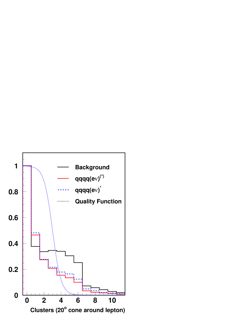
(a)	(b)

Figure 3.3: Sigmoid function used for quality calculations and an example quality variable.

The sigmoid is parameterized as $f(x;a,b,c)=\frac{1}{1+e^{\frac{-c(x-a)}{b}}}$. The parameter $a$ sets the point at which $f=\frac{1}{2}$, $b$ sets the width of the transition from 0 to 1, and $c=\pm 1$ determines whether the $f\rightarrow 0$ or $f\rightarrow 1$ as $x\rightarrow\infty$.

(a) Sigmoid function for several choices of $a$, $b$, and $c$.

(b) Example quality variable from the $\textrm{qqqqe}\nu$ subchannels. Good isolated electrons should have small numbers of calorimeter clusters around them, while electrons from semileptonic decays will be close to jets and their calorimeter clusters.

The parameters were chosen so that $f_{i}(x;a,b,c)$ is near one for good signal leptons and drops to zero for more poorly reconstructed leptons. We multiplied the results for the different variables and placed a cut at 0.1 on the product.

Besides the subchannel identification and quality requirements, we applied additional preselection cuts to remove other obvious backgrounds. To preselect hadronic events, we required 30 calorimetric clusters, 20 charged tracks, 40 GeV of energy in the BGO, and 10 GeV of energy in the HCAL. To select against single-W and $\textrm{q}\bar{\textrm{q}}(\gamma)$ backgrounds, we required the event thrust to be less than 0.9, the fraction of visible energy in a $30^{\circ}$ cone around the beampipe to be less than 60%, and $\left|\cos\theta_{{\scriptsize\textrm{missing}}}\right|<0.92$. We also required the event to contain no photons of greater than 20 GeV. Another major source of background for this channel is $\textrm{e}^{+}\textrm{e}^{-}\rightarrow\textrm{WW}\rightarrow\textrm{qql}\nu$, so we fit the event to two jets after excluding the lepton identified above and required that the dijet mass be greater than 90 GeV.

After preselection, the major remaining background was $\textrm{e}^{+}\textrm{e}^{-}\rightarrow\textrm{WW}$, particularly $\textrm{WW}\rightarrow\textrm{qqqq}$ events where one of the quarks decays semileptonically. For each subchannel, we prepared one network with the ten input variables listed in Table 3.5, twenty hidden nodes, and one output node to remove the WW and $\textrm{e}\nu\textrm{qq}$ backgrounds.

Variable	Description	Trend
$\chi_{\textrm{WW}}^{2}$	$\chi^{2}$ of a 5C fit to $\textrm{e}^{+}\textrm{e}^{-}\rightarrow\textrm{WW}\rightarrow\textrm{qqqq}$	WW background events should have a good $\chi^{2}$ for this fit, while signal events should not fit as well.
$\textrm{E}^{\textrm{max}}_{4\textrm{j}-1\textrm{l}}$	Energy of the most energetic jet from a fit to four jets, having removed the candidate lepton.
$\textrm{E}^{\textrm{min}}_{4\textrm{j}-1\textrm{l}}$	Energy of the least energetic jet from a fit to four jets, having removed the candidate lepton.	$(\textrm{l}\nu)^{*}$ signal events should have four reasonably equal jets, while many backgrounds have several high energy jets and several very low energy gluon jets. $(\textrm{l}\nu)^{(*)}$ signal events will look more like background events.
$\theta^{\textrm{min}}_{4\textrm{j}-1\textrm{l}}$	Minimum angle between any two of the four jets.	Gluon jets tend to be emitted at small angles relative to the emitting quark jet.
$m^{4c}_{\textrm{Z}}$	Mass of the dijet pair after the 4C fit with mass closest to $m_{\scriptsize\mathrm{Z}}$.	For signal events, this should be close to $m_{\scriptsize\mathrm{Z}}$.
$m^{4c}_{\textrm{L}}$	Mass of the lepton-neutrino system after the 4C fit.	For $(\textrm{l}\nu)^{*}$, this should be small, while for $(\textrm{l}\nu)^{(*)}$ it should be close to $m_{\scriptsize\mathrm{W}}$.
$m^{4c}_{\textrm{Q}}$	Mass of the other two jets after the 4C fit.	For $(\textrm{l}\nu)^{*}$, this should be close to $m_{\scriptsize\mathrm{W}}$, while for $(\textrm{l}\nu)^{(*)}$ it should be small.
$p^{4c}_{\textrm{L}}$	Momentum of the lepton-neutrino system after the 4C fit.
$p^{4c}_{\textrm{Q}}$	Momentum of the two jet system after the 4C fit.	For signal events, the momentum of the decay pairs should be small and equal.
$\log Y_{34}$	Durham Y value where the fit changes from three jets to four.	Events with gluon jets will tend to have smaller Y values.

Table 3.5: Neural network variables for the $\textrm{qqqql}\nu$ selection networks.

For the electron and muon subchannels, we cut on the network output at 0.5, while we cut the tau subchannels at 0.3. The numbers of events expected and observed in this channel are listed in Table 3.6, broken down by subchannel. We produced final discriminant distributions using the output of the neural network and the reconstructed mass separately for each subchannel.

	1999		2000		1999		2000
	Preselection	Selection	Preselection	Selection	Preselection	Selection	Preselection	Selection
	$\textrm{qqqqe}\nu$				$\textrm{qqqq}(\textrm{e}\nu)^{*}$
WW background	0.41	0.18	0.75	0.27	1.10	0.37	1.82	0.67
ZZ background	0.47	0.33	0.99	0.64	0.39	0.20	0.49	0.25
$\textrm{q}\bar{\textrm{q}}$ background	0.34	0.17	0.66	0.39	0.78	0.20	1.03	0.38
$\textrm{e}\nu\textrm{qq}$ background	0.68	0.21	1.49	0.43	0	0	0.01	0
Zee background	0.22	0.11	0.56	0.29	0.11	0.07	0.09	0.03
Total MC Bkgd	2.13	1.01	4.47	2.04	2.39	0.85	3.46	1.35
Data	4	1	4	3	2	1	3	1
Signal for $m_{\textrm{h}}=105$ GeV	0.31	0.26	0.91	0.80	0.27	0.23	0.77	0.69
	$\textrm{qqqq}\mu\nu$				$\textrm{qqqq}(\mu\nu)^{*}$
WW background	0.77	0.32	1.42	0.53	0.88	0.29	1.88	0.51
ZZ background	0.31	0.16	0.63	0.39	0.17	0.07	0.32	0.19
$\textrm{q}\bar{\textrm{q}}$ background	0.06	0.06	0.13	0.1	0.17	0.06	0.49	0.24
Total MC Bkgd	1.16	0.55	2.18	1.03	1.24	0.44	2.73	0.96
Data	1	0	1	0	0	0	1	1
Signal for $m_{\textrm{h}}=105$ GeV	0.19	0.16	0.60	0.53	0.24	0.20	0.64	0.56
	$\textrm{qqqq}\tau\nu$				$\textrm{qqqq}(\tau\nu)^{*}$
WW background	5.7	2.0	12.1	4.3	41.7	6.2	78.0	11.9
ZZ background	0.6	0.2	1.2	0.5	2.7	1.1	5.9	2.4
$\textrm{q}\bar{\textrm{q}}$ background	2.9	1.0	4.9	1.8	13.4	2.0	21.2	3.8
$\textrm{e}\nu\textrm{qq}$ background	3.9	0.7	8.2	1.7	0.6	0.1	1.2	0.31
Total MC Bkgd	13.2	4.0	26.5	8.32	58.5	9.5	106.2	18.4
Data	13	3	36	8	64	8	138	22
Signal for $m_{\textrm{h}}=105$ GeV	0.26	0.22	0.63	0.55	0.17	0.14	0.40	0.35

Table 3.6: Preselection and selection for the $\textrm{qqqql}\nu$ analysis.

3.3 The $\nu\nu\mathrm{qqqq}$ Channel

In this channel, the Z decays to neutrinos and the W’s decay hadronically, so all the visible energy in the event comes from the Higgs. The signature is two medium-energy jets with the invariant mass of the W, two low-energy jets with a much smaller invariant mass, and a missing mass of the Z. The total energy in the event should be twice the beam energy and the vector sum of all momenta in the event should be zero. Thus the missing mass is

$$m_{{\scriptsize\textrm{missing}}}=\sqrt{(\sqrt{s}-\mathrm{E}_{\scriptsize\mathrm{vis}})^{2}-p^{2}_{{\scriptsize\textrm{vis}}}}.$$

In this case, the two neutrinos produced by the Z should have an invariant mass of $m_{\scriptsize\mathrm{Z}}$.

The most important background to this channel was the $\textrm{e}^{+}\textrm{e}^{-}\rightarrow\textrm{WW}$ process, particularly the case where $\textrm{WW}\rightarrow\textrm{q}\bar{\textrm{q}}^{\prime}\tau\nu$. A tau decays hadronically 65% of the time, leaving an event with two high energy jets from the $\textrm{q}\bar{\textrm{q}}^{\prime}$ and one low energy jet from the tau. The tau decay also involves a neutrino which contributed to the missing mass. Gluon radiation or jet reconstruction can easily account for a fourth low energy jet.

Another very important background was the $\textrm{e}^{+}\textrm{e}^{-}\rightarrow\textrm{q}\bar{\textrm{q}}(\gamma\gamma)$ process, where the both the electron and positron emit a photon before annihilating, or one emits two photons. After emitting the photons, the electron and positron interact at smaller effective center-of-mass energy ($\sqrt{s}^{\prime}$). This “double-radiative” process has a sharp peak for $\sqrt{s}^{\prime}=m_{\scriptsize\mathrm{Z}}$, where the emission of the photons effectively returns the process to the huge Z resonance at 91 GeV visible in Figure 3.1. We reduced this background by requiring the event thrust to be less than 0.9, the fraction of visible energy in a $30^{\circ}$ cone around the beampipe to be less than 60%, and $\left|\cos\theta_{{\scriptsize\textrm{missing}}}\right|<0.96$.

We preselected events with substantial missing energy by requiring $0.4<\frac{\mathrm{E}_{\scriptsize\mathrm{vis}}}{\sqrt{s}}<0.7$ and chose hadronic events by requiring 20 calorimeter clusters and 10 charged tracks in the event. We also required at least 30 GeV of energy in the BGO and 10 GeV in the HCAL. To select against radiative events, we required no identified photon with more than 10 GeV of energy, less than 10 GeV of energy deposited in either the ALR or luminosity monitor, and that the missing momentum vector not be pointing toward the EGAP. We forced the event to four jets using the Durham algorithm and required at least one charged track in each jet and a minimum jet energy of 6 GeV to select against low energy jets from gluons or poor jet reconstruction.

After preselection, we prepared three networks with the eight inputs described in Table 3.7, twenty hidden nodes, and one output node.

Variable	Description	Trend
$\textrm{E}^{\textrm{max}}_{4\textrm{j}}$	Energy of the most energetic jet from a fit to four jets.
$\textrm{E}^{\textrm{min}}_{4\textrm{j}}$	Energy of the least energetic jet from a fit to four jets.	Signal events tend to have two medium-energy and two low-energy jets, while backgrounds will tend to have higher $\textrm{E}^{\textrm{max}}$ values and lower $\textrm{E}^{\textrm{min}}$ values.
$\theta^{\textrm{min}}_{4\textrm{j}}$	Minimum angle between any two of the four jets.	Gluon jets tend to be emitted at small angles relative to the emitting quark jet.
$\alpha_{\textrm{W}^{(*)}\textrm{W}^{*}}$	Angle between the decay planes of the W candidate and $\textrm{W}^{*}$ candidate.	This angle is likely to be smaller for gluon jets which fake the $\textrm{W}^{*}$.
$m^{5c}_{\textrm{W}}$	Mass of the dijet with invarient mass closest to $m_{\scriptsize\mathrm{W}}$after the 5C fit.	For signal events, this mass should be close to $m_{\scriptsize\mathrm{W}}$.
$m_{\textrm{recoil}}$	Recoil mass of the event.	For signal events, the recoil mass should be $m_{\scriptsize\mathrm{Z}}$. Background events will tend to have smaller recoil mass.
$\log Y_{23}$	Durham Y value where the fit changes from two jets to three.
$\log Y_{34}$	Durham Y value where the fit changes from three jets to four.	Events with gluon jets will tend to have smaller Y values.

Table 3.7: Neural network variables for the $\nu\nu\textrm{qqqq}$ selection networks.

One network was trained to reject WW and $\textrm{e}\nu\textrm{qq}$ backgrounds, a second to reject ZZ, and a third to remove $\textrm{q}\bar{\textrm{q}}(\gamma)$. We used only the $\textrm{h}\rightarrow\textrm{WW}$ signal for training, not the $\textrm{h}\rightarrow\textrm{ZZ}$. At the selection stage, we required ${\cal N}_{\scriptsize\ \mathrm{WW}}>0.4$, ${\cal N}_{\scriptsize\ \mathrm{ZZ}}>0.4$, and ${\cal N}_{\scriptsize\ \mathrm{q\bar{q}}}>0.6$. The numbers of predicted and observed events after preselection and selection are given in Table 3.8.

	1999		2000
	Preselection	Selection	Preselection	Selection
WW background	94.1	10.2	169.1	21.3
ZZ background	8.0	1.9	17.3	3.0
qq background	32.3	2.6	43.6	4.3
$\textrm{e}\nu\textrm{qq}$ background	26.1	1.3	47.5	3.1
Total MC	161.1	16.0	278.6	31.9
Data	147	13	304	28
Signal for $m_{\textrm{h}}=105$ GeV	1.04	0.84	2.93	2.52

Table 3.8: Preselection and selection totals for the $\nu\nu\textrm{qqqq}$ channel.

As in the qqqqqq channel, we can add $\textrm{hZ}\rightarrow\textrm{Z}^{(*)}\textrm{Z}^{*}\textrm{Z}\rightarrow\nu\nu\textrm{qqqq}$ events to our base $\textrm{h}\rightarrow\textrm{WW}$ signal. Of course, any of the three Z bosons can be the one which decays to the neutrino pair, not only the Higgsstrahlung Z. Fortunately, the kinematics of the event minimize the error on the Higgs mass generated by taking $\textrm{Z}^{(*)}\rightarrow\nu\nu$ instead of the Higgsstrahlung $\textrm{Z}\rightarrow\nu\nu$. The selection accepted events where either the radiated Higgsstrahlung Z or the $\textrm{Z}^{(*)}$ from the Higgs decayed to neutrinos, but the missing energy in the $\textrm{Z}^{*}\rightarrow\nu\nu$ case was too small. The accepted signatures made up 20% of the total $\textrm{hZ}\rightarrow\textrm{ZZZ}$ branching fraction, and including them increased the expected channel signal rate by 15%.

3.4 The $\nu\nu\mathrm{qql}\nu$ Channel

In the $\nu\nu\textrm{qql}\nu$ channel, the Z decays to neutrinos, while one W decays leptonically and the other into quarks. In this channel, there are not enough constraints to reconstruct the Higgs mass directly, so the channel is mostly a counting experiment. As in the $\textrm{qqqql}\nu$ channel, the signal divides into six subchannels as a function of the lepton flavor and source ( $\textrm{W}^{(*)}$ or $\textrm{W}^{*}$). We used the same variables to separate the two channels and similar lepton quality requirements as in the $\textrm{qqqql}\nu$ analysis. We required a minimum quality value as the basic level of preselection.

The visible energy in this channel is quite small compared to the other channels, since there are at least three energetic neutrinos in the event. The low visible energy means that two-photon processes become important sources of background and several cuts are applied to eliminate them. A particularly useful variable for reducing the two-photon and $\textrm{q}\bar{\textrm{q}}(\gamma)$ backgrounds was $\sin\Psi\equiv\left|\left(\hat{j}_{1}\times\hat{j}_{2}\right)\cdot\hat{z}\right|$, where $\hat{j}_{1}$ and $\hat{j}_{2}$ are the unit vectors along the directions of the jets determined from fitting the event into a two-jet topology. This variable preferentially selects events in which the jets are at right angles to each other and to the beampipe. Many background events have back-to-back jets or jets with small angles relative to the beampipe. We required events to have $\sin\Psi>0.07$.

For preselection, we also required $\left|\cos\theta_{{\scriptsize\textrm{missing}}}\right|<0.9$, the fraction of visible energy in a $30^{\circ}$ cone around the beampipe to be less than 40%, and that there be less than 7 GeV of energy in the ALR. We also set cuts on the BGO energy, recoil mass, and numbers of clusters and tracks on a subchannel-basis as given in Table 3.9.

Quantity	$\nu\nu\textrm{qq}(\textrm{e}\nu)$	$\nu\nu\textrm{qq}(\mu\nu)$	$\nu\nu\textrm{qq}(\tau\nu)$
BGO Energy/$\sqrt{s}$	0.14 < x < 0.4	0.02 < x < 0.22	0.02 < x < 0.3
Calorimeter clusters	10 < x < 80	10 < x < 75	10 < x < 80
Charge tracks	4 < x < 23	3 < x < 25	5 < x < 25
Recoil mass	> 95 GeV	> 80 GeV	> 115 GeV
	$\nu\nu\textrm{qq}(\textrm{e}\nu)^{*}$	$\nu\nu\textrm{qq}(\mu\nu)^{*}$	$\nu\nu\textrm{qq}(\tau\nu)^{*}$
BGO Energy/$\sqrt{s}$	0.1 < x < 0.42	0.05 < x < 0.35	0.05 < x < 0.4
Calorimeter clusters	15 < x < 80	10 < x < 80	15 < x < 85
Charge tracks	6 < x < 33	5 < x < 35	5 < x < 33
Recoil mass	> 80 GeV	> 80 GeV	> 75 GeV

Table 3.9: Subchannel-specific preselection cuts for $\nu\nu\textrm{qql}\nu$.

The most important background was $\textrm{e}^{+}\textrm{e}^{-}\rightarrow\textrm{WW}\rightarrow\textrm{qql}\nu$, particularly the $\textrm{WW}\rightarrow\textrm{qq}\tau\nu$ channel. We reconstructed an average W pair mass to help reject this background. First, we scaled the energies and masses of the two jets by a common factor until the sum of their energies was $\frac{\sqrt{s}}{2}$, as would be the case in a real WW event. Then, we constructed a “neutrino” to balance the event. We calculated $m_{\scriptsize\mathrm{W}}^{{\scriptsize\textrm{recon}}}$ as the average of the invariant mass of the “neutrino” - lepton system and the scaled di-jet invariant mass. We used this variable along with several others listed in Table 3.10 to prepare one $8\times 20\times 1$ neural network for each subchannel.

Variable	Description	Trend
$\frac{E_{l}}{\sqrt{s}}$	Energy of the candidate lepton normalized to $\sqrt{s}$.	Lepton energy for the $(\textrm{l}\nu)^{*}$channel will be small, while in the $(\textrm{l}\nu)^{(*)}$ channel it will be larger.
$\frac{E_{{\scriptsize\textrm{jet}1}}+E_{{\scriptsize\textrm{jet}2}}}{\sqrt{s}}$	Jet energy sum scaled by the center-of-mass energy.	The jet energy is complementary to the lepton energy - larger for $(\textrm{l}\nu)^{*}$and smaller for $(\textrm{l}\nu)^{(*)}$.
$\alpha$	Angle between the plane containing the two jets and the lepton.	Leptons from quark decay backgrounds will tend to lie in the plane of the jets.
$\theta^{\textrm{min}}_{\textrm{jl}}$	Minimum angle between either jet and the candidate lepton.	Leptons from quark decay will tend to be close in angle to a jet.
$\theta_{\textrm{lm}}$	Angle between the lepton and missing momentum vector.	For semi-leptonic WW events, the direction angle between the lepton and missing momentum should coorespond to the W mass. For other backgrounds, this angle should have no particular value. For signal, we expect some coorelation between the lepton and missing energy.
$m_{\scriptsize\mathrm{W}}^{{\scriptsize\textrm{recon}}}$	Average mass for the $\textrm{WW}\rightarrow\textrm{qql}\nu$ reconstruction.	This mass should be close to $m_{\scriptsize\mathrm{W}}$ for semileptonic WW background events.
$m_{{\scriptsize\textrm{missing}}}$	Recoil mass against the visible part of the event.	For signal events, the recoil mass should be $m_{\scriptsize\mathrm{Z}}$, but energy losses from the third neutrino and in the jets mean that the observed missing mass will be > $m_{\scriptsize\mathrm{Z}}$. Background events will tend to have a smaller recoil mass.
$m_{\textrm{jj}}$	Dijet mass.	For $(\textrm{l}\nu)^{(*)}$ signal events, this will peak around 25 GeV, depending on $m_{\scriptsize\mathrm{h}}$. This variable is not used for $(\textrm{l}\nu)^{*}$networks.

Table 3.10: Neural network variables for the $\nu\nu\textrm{qql}\nu$ selection networks.

For final selection, we placed cuts on ${\cal N}$ around $0.35$, depending on the subchannel. The numbers of events predicted and observed after selection and preselection are listed in Table 3.11. There were insufficient constraints to fully reconstruct the Higgs mass, so we used the visible mass as the final variable, as it was quite correlated with the Higgs mass.

	1999		2000
	$\nu\nu\textrm{qq}(\textrm{e}\nu)+\nu\nu\textrm{qq}(\mu\nu)+\nu\nu\textrm{qq}(\tau\nu)$
	Preselection	Selection	Preselection	Selection
WW background	1.9	0.3	3.8	0.7
ZZ background	0.5	<0.1	0.7	0.0
qq background	0.1	<0.1	0.3	0.0
$\textrm{e}\nu\textrm{qq}$ background	1.2	0.2	2.7	0.5
Total MC	3.7	0.5	7.6	1.2
Data	6	0	15	2
Signal for $m_{\textrm{h}}=105$ GeV	0.29	0.24	0.67	0.60
	$\nu\nu\textrm{qq}(\textrm{e}\nu)^{*}+\nu\nu\textrm{qq}(\mu\nu)^{*}$
WW background	11.2	1.2	23.2	2.7
ZZ background	1.4	0.1	2.2	0.4
qq background	0.4	<0.1	0.5	<0.1
$\textrm{e}\nu\textrm{qq background}$	1.6	0.2	3.8	0.7
Total MC	14.6	1.5	29.8	3.8
Data	15	1	24	6
Signal for $m_{\textrm{h}}=105$ GeV	0.19	0.17	0.43	0.40

Table 3.11: Preselection and selection totals for the $\nu\nu\textrm{qql}\nu$ channel.

3.5 The llqqqq Channel

In this channel, the Z decays to a pair of electrons or muons, while the W’s decay hadronically. The decay of the Z to taus was not considered in the analysis. The BGO and muon chambers give very good resolution on the leptons from the Z decay, so the Z was very well reconstructed and the Higgs mass could be determined from the recoil. The only difficulty with this channel was its small branching ratio, which implied a small number of expected signal events. The event signature is two energetic leptons with the invariant mass of the Z, two energetic jets with about $m_{\scriptsize\mathrm{W}}$, and two smaller jets.

The requirement that the two leptons have an invariant mass close to $m_{\scriptsize\mathrm{Z}}$ removed almost all background events which did not contain legitimate Z bosons. At least one of the leptons in the rejected events generally came from semileptonic quark decay in a jet. The most important remaining background was Z pair production, but good recoil mass resolution allowed the suppression of this background except for $m_{\scriptsize\mathrm{h}}\sim m_{\scriptsize\mathrm{Z}}$.

The first phase of the analysis was identification of the two leptons considered to be the decay products of the Z. The analysis calculated quality values for each pair of identified leptons, considering both the single lepton factors, such as minimum angle to a jet, as well as di-lepton factors such as $\left|m_{\scriptsize\mathrm{Z}}-m_{ll}\right|$. Pairs such as $\mu\textrm{e}$ which would not arise from Z decay were not considered. The pair with the best quality factor was chosen as the candidate pair. This assignment put each event into either the eeqqqq or $\mu\mu\textrm{qqqq}$ subchannel or rejected it.

After the identification, several preselection cuts were applied to select events consistent with slightly more than two jets, while removing as much of the four-jet background as possible. We required at least 30 calorimeter clusters and between 10 and 40 charged tracks in the event. We required $5\textrm{ GeV}<\mathrm{E}_{\scriptsize\mathrm{HCAL}}<65\textrm{ GeV}$, and $0.4<\frac{\mathrm{E}_{\scriptsize\mathrm{BGO}}}{\sqrt{s}}<0.9$ for eeqqqq events and $0.1<\frac{\mathrm{E}_{\scriptsize\mathrm{BGO}}}{\sqrt{s}}<0.5$ for $\mu\mu\textrm{qqqq}$. Since there were no neutrinos in our event signature, we required $0.8<\frac{\mathrm{E}_{\scriptsize\mathrm{vis}}}{\sqrt{s}}<1.2$ for eeqqqq events and $0.7<\frac{\mathrm{E}_{\scriptsize\mathrm{vis}}}{\sqrt{s}}<1.2$ for $\mu\mu\textrm{qqqq}$ events.

After preselection, we applied a 4C fit requiring energy and momentum conservation and then applied a few selection cuts. We required the $\chi^{2}$ of the 4C fit to be less than 3 for eeqqqq and less than 4.5 for $\mu\mu\textrm{qqqq}$ and that the reconstructed Z mass was between 60 GeV and 110 GeV. We also forced the event to a four-jet + two lepton topology and required the $\log Y_{34}$ determined from the fit be larger than -7.5. These cuts removed the remaining “obvious” backgrounds, and then we trained three neural networks to remove the remaining background: one for the eeqqqq subchannel and two for $\mu\mu\textrm{qqqq}$. The eeqqqq neural network and one of the $\mu\mu\textrm{qqqq}$ networks were trained against the ZZ and Zee backgrounds. The second $\mu\mu\textrm{qqqq}$ network was trained against WW and $\textrm{e}\nu\textrm{qq}$ backgrounds. The six variables used in these $6\times 25\times 1$ neural networks are listed in Table 3.12.

Variable	Description	Trend
$\textrm{E}^{\textrm{max}}_{4\textrm{j}-2\textrm{l}}$	Energy of the most energetic jet from a fit to four jets.
$\textrm{E}^{\textrm{min}}_{4\textrm{j}-2\textrm{l}}$	Energy of the least energetic jet from a fit to four jets.	Signal events tend to have two medium-energy and two low-energy jets, while backgrounds will tend to have higher $\textrm{E}^{\textrm{max}}$ values and lower $\textrm{E}^{\textrm{min}}$ values.
$\theta^{\textrm{min}}_{\textrm{jj}}$	Minimum angle between any two of the four jets.	Gluon jets tend to be emitted at small angles relative to the emitting quark jet.
$\theta^{\textrm{min}}_{\textrm{jl}}$	Minimum angle between any jet and any lepton.	Backgrounds where the lepton is produced from quark decay will tend to have smaller values of $\theta^{\textrm{min}}_{\textrm{jl}}$ than signal events.
$m_{\textrm{ll}}$	Di-lepton invarient mass of the event.	For signal events, the dilepton mass should be $m_{\scriptsize\mathrm{Z}}$. Background events where the leptons are not from a Z will tend to have a smaller dilepton mass.
$\log Y_{34}$	Durham Y value where the fit changes from three jets to four.	Events with gluon jets will tend to have smaller Y values.

Table 3.12: Neural network variables for the llqqqq selection networks.

We required that selected events have ${\cal N}_{\scriptsize\ \mathrm{ZZ}}>0.25$ and ${\cal N}_{\scriptsize\ \mathrm{WW}}>0.2$(for $\mu\mu\textrm{qqqq}$). The number of background and signal events expected and data events observed after preselection and selection are given in Table 3.13.

	1999		2000
	Preselection	Selection	Preselection	Selection
	eeqqqq
ZZ background	2.2	0.7	4.6	1.6
Zee background	0.6	0.1	1.1	0.5
$\textrm{e}\nu\textrm{qq}$ background	0	0	0.1	0
Total MC	2.8	1.1	5.8	2.1
Data	1	0	3	2
Signal for $m_{\textrm{h}}=105$ GeV	0.11	0.10	0.31	0.29
	$\mu\mu\textrm{qqqq}$
ZZ background	2.4	0.9	4.5	1.9
WW background	3.4	0.8	6.1	1.1
qq background	0.5	0	0.7	0.1
Total MC	6.3	1.7	11.3	3.1
Data	5	2	12	4
Signal for $m_{\textrm{h}}=105$ GeV	0.12	0.10	0.29	0.27

Table 3.13: Preselection and selection totals for the llqqqq channel.

The llqqqq channel was also able to benefit from a matching signature in $\textrm{h}\rightarrow\textrm{ZZ}$. However, signal Monte Carlo was not available for this process. Since the efficiency and shape for the $\textrm{h}\rightarrow\textrm{ZZ}$ in both the $\nu\nu\textrm{qqqq}$ and qqqqqq channels matched the $\textrm{h}\rightarrow\textrm{WW}$, we simply increased the cross-section for this channel by the appropriate factor to account for the case where Higgsstrahlung Z decayed leptonically. Without signal Monte Carlo, we cannot properly adjust for the case where one of the Higgs decay Z bosons decays leptonically.

3.6 The $\mathrm{qql}\nu\mathrm{l}\nu$ Channel

In the $\textrm{qql}\nu\textrm{l}\nu$ channel, the Z decays hadronically while both W bosons decay to lepton-neutrino pairs. The analysis was lepton-flavor blind, except for lepton quality cuts which were flavor-specific. We required two identified leptons, one with more than 12 GeV of energy and the second with energy greater than 10 GeV. We accepted electrons, muons, or taus, but did not accept minimum-ionizing particle (MIP) candidates as muons or taus.

At the preselection level, we required $0.5<\frac{\mathrm{E}_{\scriptsize\mathrm{vis}}}{\sqrt{s}}<0.85$, since the neutrinos should not carry away more than approximately 40% of the center-of-mass energy. To select events with hadronic content, we required 25 calorimetric clusters, 8 tracks, at least 30 GeV of energy in the BGO, and at least 8 GeV in the HCAL. To remove two-photon and $\textrm{q}\bar{\textrm{q}}(\gamma)$ backgrounds, we required $\left|\cos\theta_{{\scriptsize\textrm{missing}}}\right|<0.92$, an event thrust of less than 0.93, less than 40% of the total visible energy within $30^{\circ}$ of the beampipe, and there be no photon in the event with more than 20 GeV of energy. To remove unmodeled or poorly modeled backgrounds, we required less than 10 GeV in the ALR or luminosity monitor.

After preselection, the dominant backgrounds were W pair production and $\textrm{e}^{+}\textrm{e}^{-}\rightarrow\textrm{e}\nu\textrm{q}\bar{\textrm{q}}$ processes. To remove these backgrounds, we constructed an $8\times 16\times 1$ neural network using the variables listed in Table 3.14.

Variable	Description	Trend
$\textrm{m}_{2\textrm{j}-2\textrm{l}}$	Invarient mass of the two jets after the fit removing the identified leptons.	For signal events, this should be close to $m_{\scriptsize\mathrm{Z}}$, while for WW background it will less than $m_{\scriptsize\mathrm{W}}$.
$\theta^{\textrm{min}}_{\textrm{jj}-\textrm{L}}$	Minimum angle between the more energetic lepton and either of the two jets.
$\theta^{\textrm{min}}_{\textrm{jj}-\textrm{l}}$	Minimum angle between the less energetic lepton and either of the two jets.	Leptons from quark decay in jets tend to be emitted at small angles relative to the emitting jet.
$m^{\textrm{scale}}_{\textrm{jj}}$	Dijet mass from the fit to two jets and one lepton after scaling the energies and masses of the jets by a common factor until $\sum\textrm{E}_{\textrm{j}}=\sqrt{s}$.	For WW background events, the dijet mass should be $m_{\scriptsize\mathrm{W}}$, while it should be considerably larger for signal events.
$m_{\textrm{l}\nu}^{\textrm{scale}}$	Invarient mass of the lepton-missing momentum system after scaling the jets.	For WW background events, this mass should also be $m_{\scriptsize\mathrm{W}}$.
$\theta_{\textrm{ll}}$	Lepton-lepton angle.	For signal events, both leptons should be in the same hemisphere, while background leptons tend to be at higher angles.
$\log\frac{Y_{23}}{Y_{34}}$	Ratio of the Durham Y value where the fit changes from two jets to three to the Y value for three to four.	A signal event will appear either three-jet-like or four-jet-like depending on the direction and energy of the second lepton, while many background events will be two-jet or four-jet.

Table 3.14: Neural network variables for the $\textrm{qql}\nu\textrm{l}\nu$ selection networks.

We required ${\cal N}>0.5$ for selection. The numbers of expected background and signal and observed data after preselection and selection are given in Table 3.15.

	1999		2000
	Preselection	Selection	Preselection	Selection
	$\textrm{qql}\nu\textrm{l}\nu$ without taus
WW background	4.26	0.22	6.40	0.32
$\textrm{e}\nu\textrm{qq}$ background	3.11	0.12	4.53	0.09
ZZ background	0.56	0.19	1.06	0.36
qq background	0.58	0	0.55	0.02
Total MC	8.62	0.55	12.74	0.86
Data	7	0	16	2
Signal for $m_{\textrm{h}}=105$ GeV	0.15	0.09	0.58	0.36
	$\textrm{qql}\nu\textrm{l}\nu$ with taus
WW background	23.6	5.6	33.7	7.5
$\textrm{e}\nu\textrm{qq}$ background	8.6	2.3	12.2	2.3
qq background	2.7	0.6	4.0	0.9
ZZ background	2.5	1.3	3.9	2.2
Total MC	37.6	10.0	54.1	13.1
Data	34	9	62	19
Signal for $m_{\textrm{h}}=105$ GeV	0.22	0.15	0.41	0.28

Table 3.15: Preselection and selection totals for the $\textrm{qql}\nu\textrm{l}\nu$ channel.

After selection, we separated the events into two groups: events where neither lepton was identified as a tau and events where at least of one of the leptons was identified as a tau. The amount of background in the second group was much larger than in the first. We created discriminant final variables for these two subchannels separately, using the reconstructed Higgs mass and the network output. We reconstructed the Higgs mass by scaling the jet masses and energies by a common factor until $m_{jj}=m_{\scriptsize\mathrm{Z}}$, and then calculating the recoil mass off the di-jet.

Chapter 4 Results of the Search

Attempt the end, and never stand to doubt;
Nothing’s so hard but search will find it out.

Robert Herrick

4.1 Search in the Two Photon Channel

All four LEP collaborations have performed searches for a Higgs decaying to two photons using the Higgsstrahlung production mode. The details of each experiment’s analysis are given in journal articles[36, 37, 38, 39, 40], but the general strategies will be outlined here.

The decays of the Z define three search channels: $\textrm{hZ}\rightarrow\gamma\gamma\textrm{q}\bar{\textrm{q}}$, $\textrm{hZ}\rightarrow\gamma\gamma\nu\bar{\nu}$, and $\textrm{hZ}\rightarrow\gamma\gamma\textrm{l}^{+}\textrm{l}^{-}$. For all the channels, the major background is double-radiative Z production as described in Section 3.3. The process tends to produce on-shell, boosted Z bosons and one or more high energy photons that mimic the signal. For the signal, the di-photon spectrum peaks at the Higgs mass, while the background spectrum is fairly flat over a wide range of invariant masses.

In general, photons are experimentally identified as isolated clusters in the electromagnetic calorimeters with no matching track to indicate an electron. Additional selection criteria are also used to reject merged $\pi_{0}$’s and other possible sources of fakes.

DELPHI, L3, and OPAL have developed analyses for each of the three search channels separately, using similar cut-based approaches to reduce the background. In contrast, the ALEPH experiment performs a “global” analysis, focusing on the di-photon system and combining all the Z decay channels together. The results from these selections are presented in Table 4.1.

	Energy		Expected	Benchmark	Expected
Experiment	Range	Candidates	Bkgd	Limit (GeV)	Limit (GeV)
ALEPH	192-209	10	10.8	104.4	104.6
DELPHI	189-209	47	42.2	103.6	105.1
L3	189-209	64	69.5	104.1	104.9
OPAL	88-209	184	185.7	104.8	105.2
LEP		305	308.5	106.5	109.6

Table 4.1: Results of the $\textrm{h}\rightarrow\gamma\gamma$ search.

Each experimental group provides data, background, and predicted signal distributions of the reconstructed Higgs mass to the LEP Higgs Working Group (LHWG). These distributions, added together, are plotted in Figure 4.1 for a mass hypothesis of $m_{\textrm{h}}=100\textrm{ GeV}$.

Figure 4.1: Mass distribution of selected events in the LEP combined $\textrm{h}\rightarrow\gamma\gamma$ search.

The results can also be statistically combined to produce limits or indicate the presence of signal.

4.2 Hypothesis Testing and Limit Setting

In January of 2000, just before the last year of LEP, CERN hosted a workshop to discuss the best way to derive confidence level limits and combine the results from different experiments and search channels [41]. In the Standard Model search, there are four physical channels and at least nine center of mass energies. Thus, there are 36 independent channels to combine from each of the four experiments. To obtain the maximum search power from the analyses, the goal is to consider the shape of the final variables, rather than just execute a global counting experiment. The solution is to consider each bin of each final variable as a separate counting experiment in the form of a log-likelihood ratio:

$$L_{i}=s_{i}-n_{i}\ln\left(\frac{b_{i}+s_{i}}{b_{i}}\right)=s_{i}-n_{i}\ln\left(1+\frac{s_{i}}{b_{i}}\right)$$

where $s_{i}$, $b_{i}$, and $n_{i}$ are the number of expected signal events, expected background events, and observed events in the $i\textrm{th}$ bin, respectively. The ratio compares the data to the hypotheses of background only and signal+background. We can combine bins, center-of-mass energies, and channels simply by adding the log-likelihood ratio values for each bin. The specific form of the statistical estimator chosen by the LHWG is

$$-2\ln Q=2\sum_{i}s_{i}-2\sum_{i}n_{i}\ln\left(1+\frac{s_{i}}{b_{i}}\right).$$

A positive value of $-2\ln Q$ indicates the observed data agrees better with the background-only hypothesis, while a negative value favors the signal plus background hypothesis. The expected values of $-2\ln Q$ in the presence and absence of signal can be obtained by replacing $n_{i}$ with $s_{i}+b_{i}$ and $b_{i}$ respectively. The prefactor was chosen so that in the large number limit, $-2\ln Q\rightarrow\chi^{2}$. Both signal and background are calculated in terms of efficiencies $\epsilon^{s}_{i}$ and $\epsilon^{b}_{i}$ and the number of expected events is extracted by multiplying by the signal and background cross-sections and the luminosity. This means that $-2\ln Q$ scales linearly with luminosity, so the performance gain expected from additional luminosity is easily calculated. Also, the significance of a bin is entirely captured by its signal-to-background ratio, so we can collect bins of similar signal-to-background ratio together to speed the computation.

A single round of computations generates the observed and expected estimator values, but to gauge the importance of any excess or deficit, we determined the range of estimator values consistent with the observation. To determine this range, we create two new distributions from the signal and background distributions by replacing the value in each bin with a value drawn from the Poisson distribution with the expected value of the original bin value. These new distributions simulate what might be observed in a real experiment, as a Monte Carlo trial. We recorded the $-2\ln Q$ values from these distributions and repeat the process 50,000 or more times. The result of these trials is new statistical distributions of $-2\ln Q$.

In Figure 4.2 are the $-2\ln Q$ trial distributions from the $\textrm{h}\rightarrow\gamma\gamma$ search for $m_{\textrm{h}}=106\textrm{ GeV}$.

Figure 4.2: Example of the Background-only and Signal+Background $-2\ln Q$ distributions.

The solid black and gray curves are the $-2\ln Q$ distributions for the signal+background and background only hypotheses, respectively. The dashed line indicates the observed value calculated from the data. Two important confidence levels can be immediately obtained from this plot. The fractional area of the signal+background curve above the observed line indicates the observed confidence level for signal. In the presence of signal, one would expect $\mathrm{CL}_{\scriptsize\mathrm{s+b}}\approx\frac{1}{2}$. Very small values of $\mathrm{CL}_{\scriptsize\mathrm{s+b}}$ statistically exclude the presence of signal. Underfluctuations in data may cause anomolously small values of $\mathrm{CL}_{\scriptsize\mathrm{s+b}}$, so the LHWG exclusion crition is based on a modified confidence level $\mathrm{CL}_{\scriptsize\mathrm{s}}\equiv\frac{\mathrm{CL}_{\scriptsize\mathrm{s+b}}}{\mathrm{CL}_{\scriptsize\mathrm{b}}}$. The second confidence level in the plot is the fractional area of the background-only plot below the observed line, which gives $1-\mathrm{CL}_{\scriptsize\mathrm{b}}$. For data that contains no signal events, $\mathrm{CL}_{\scriptsize\mathrm{b}}$ should be near $\frac{1}{2}$. However, in the presence of a signal $1-\mathrm{CL}_{\scriptsize\mathrm{b}}$ will become very small. An extremely small $1-\mathrm{CL}_{\scriptsize\mathrm{b}}$ ($<5\times 10^{-7}$) is the criterion for the discovery of the Higgs boson.

4.3 Results of the Two-Photon Search

In the benchmark model, we can calculate the $-2\ln Q$ distributions using inputs provided by all four experiments. To visualize the results as a function of mass, we plot the central value of the $-2\ln Q$ distributions for the signal+background hypothesis and the background-only hypothesis as a functions of mass using dashed lines. Then we indicate the $\pm 1\sigma$ and $\pm 2\sigma$ edges from the Monte Carlo trials by shaded regions. Finally, we indicate the observed $-2\ln Q$ values using a solid line. The results of the $\textrm{h}\rightarrow\gamma\gamma$ search are shown in this form in Figure 4.3a. Where the line is in the upper half of the plot, the observation favors the background-only hypothesis and where it is in the lower it favors the signal+background. The shaded regions indicate the level of compatibility between the observed and either hypothesis. At each mass, a “cross-section” vertically through the plot would reveal distributions similar to Figure 4.2.

(a)	(b)
Figure 4.3: Results and limits for the LEP combined $\textrm{h}\rightarrow\gamma\gamma$ search. (a) $-2\ln Q$ results for the benchmark model (b) CL limits for the benchmark model (c) Branching-Ratio limits	(c)

To determine the exclusion levels as a function of mass, we can perform the $\mathrm{CL}_{\scriptsize\mathrm{s+b}}$ integration on each $-2\ln Q_{{\scriptsize\textrm{s}+\textrm{b}}}$ distribution. Using the $-2\ln Q_{{\scriptsize\textrm{b}}}$ distribution, we can also determine the median expected exclusion and the $\pm 1\sigma$ and $\pm 2\sigma$ bands. The results of this calculation are shown in Figure 4.3b. This plot shows an observed 95% CL limit on the benchmark fermiophobic Higgs at $\textrm{m}_{\textrm{h}}=106.5\textrm{ GeV}$ with a expected limit of $\textrm{m}_{\textrm{h}}=109.6\textrm{ GeV}$. These numbers are not identical to those presented by the LHWG because of the use of a different statistical method than that usually employed in the fermiophobic results. There is an excess in signal events observed above background in the high-mass region, but this excess is well within the $\pm 2\sigma$ band.

We can derive model-independent results by scaling up and down the predicted signal cross-section until $\mathrm{CL}_{\scriptsize\mathrm{s}}$ = 95%. This provides a limit on the rate of the production of any Higgs which decays to $\gamma\gamma$, regardless of model. We show the results of this calculation in Figure 4.3c along with the predictions of two models. The upper dotted line shows the prediction of the benchmark model, while the lower dotted line shows the prediction of the Standard Model. The LEP combined $\textrm{h}\rightarrow\gamma\gamma$ results can exclude the benchmark model over a large mass range, but cannot exclude the Standard Model at any mass.

4.4 Results of the $\textrm{h}\rightarrow\textrm{WW}/\textrm{ZZ}$ Search

After all analysis cuts were applied in Chapter 3, the final output of each analysis was a set of final variable distributions for data, predicted background, and signal as a function of Higgs mass hypothesis. These final variable distributions were the “inputs” to the hypothesis-testing and limit-setting algorithms. These distributions are quite complicated, so they can be visualized in several different ways.

The final variable distributions for a given mass are most conveniently plotted by grouping together bins of the final variable which have the same signal-to-background ratio, since the log-likelihood ratio uses only the signal-to-background ratio. To give a sense of the mass-dependence of the analyses, the final variable distributions for each analysis are given for two different mass hypotheses: $m_{\scriptsize\mathrm{h}}$=100 GeV and $m_{\scriptsize\mathrm{h}}$=110 GeV. Most analyses show better signal-to-background ratio for the higher mass hypothesis even though the Higgsstrahlung cross-section is larger for the lower masses. This behavior arises because background events tend to have low reconstructed “Higgs masses,” usually close to $m_{\scriptsize\mathrm{W}}$ or $m_{\scriptsize\mathrm{Z}}$.

The final results of the analysis can also be viewed using a plot of reconstructed Higgs mass directly. In such a plot, any additional information about the “signal-ness” of an event is lost, so the search sensitivity of the plot is limited. Each channel with a reconstructed mass variable (all the channels except $\nu\nu\textrm{qql}\nu$) has a plot of the reconstructed mass for all data and background events along with the signal distribution for a single mass.

The plotting technique with the highest information density is the $-2\ln Q$ plot. These plots show the expected and observed results as a continuous function of Higgs mass hypothesis. Each channel has a $-2\ln Q$ plot, but the scale used is channel-dependent. Each of $-2\ln Q$ plots also has a dark band surrounding the observed line which indicates the magnitude of the systematic error estimated for the channel. We determine the systematic errors by shifting variables in the the signal and background events while keeping the discriminant probability density functions constant. The change in $-2\ln Q$ from the normal results indicates the magnitude of the systematic error. More details of the calculation as well as tables of the major systematic errors channel are given in Appendix B.

We can compare the relative search power of the channels in various ways. In the log-likelihood plot, the $\Delta(-2\ln Q)$ distance between the background-only and signal+background hypotheses is larger for channels and mass hypotheses which have greater search power. Another is a table of the signal-to-background ratio for given number of expected signal events, as in Table 4.2. For each channel, we integrate the final variable distribution from the largest signal-to-background ratio until we reach 0.1, 0.5, and 1.0 expected events. For each expectation we report the signal-to-background ratio. Some channels never expect as many as 0.5 or 1.0 events at $m_{\scriptsize\mathrm{h}}$=110 GeV for any signal-to-background ratio.

	s/b ratio			Total expected
Channel	1.0 signal events	0.5 signal events	0.1 signal events	signal events
qqqqqq	0.14	0.22	0.24	8.05
$\textrm{qqqql}\nu$	0.75	1.8	3.7	2.71
$\nu\nu\textrm{qqqq}$	0.14	0.43	1.1	1.47
$\nu\nu\textrm{qql}\nu$	-	0.12	1.1	0.79
llqqqq	-	-	4.7	0.38
$\textrm{qql}\nu\textrm{l}\nu$	-	-	5.1	0.47

Table 4.2: Comparison of the channels by signal to background ratio for $m_{\scriptsize\mathrm{h}}$=110 GeV.

Cases where a channel expects less than 1.0 or 0.5 events total are indicated by a dash.

4.4.1 Results by Channel

The largest total number of signal events is expected in the qqqqqq channel (Figure 4.4). However, the analysis has no bin with a signal-to-background ratio greater than $\frac{1}{4}$, which is quite low compared to the other channels. The six broad jets of the fully hadronic events are difficult to reconstruct in the L3 detector, which leads to a very poor resolution on the reconstructed Higgs mass. As seen in Figure 4.4d, the channel exhibits a small constant deficit in data relative to the Standard Model background expectation, which follows directly from the small observed counting deficit (443 with 446 expected) and the wide resolution.

(a) Final variable rebinned in s/b for $m_{\textrm{h}}=100$ GeV	(b) Final variable rebinned in s/b for $m_{\textrm{h}}=110$ GeV
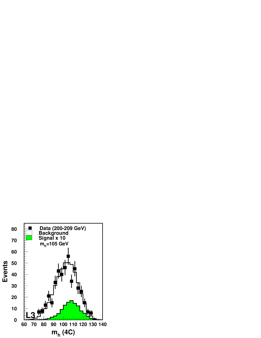
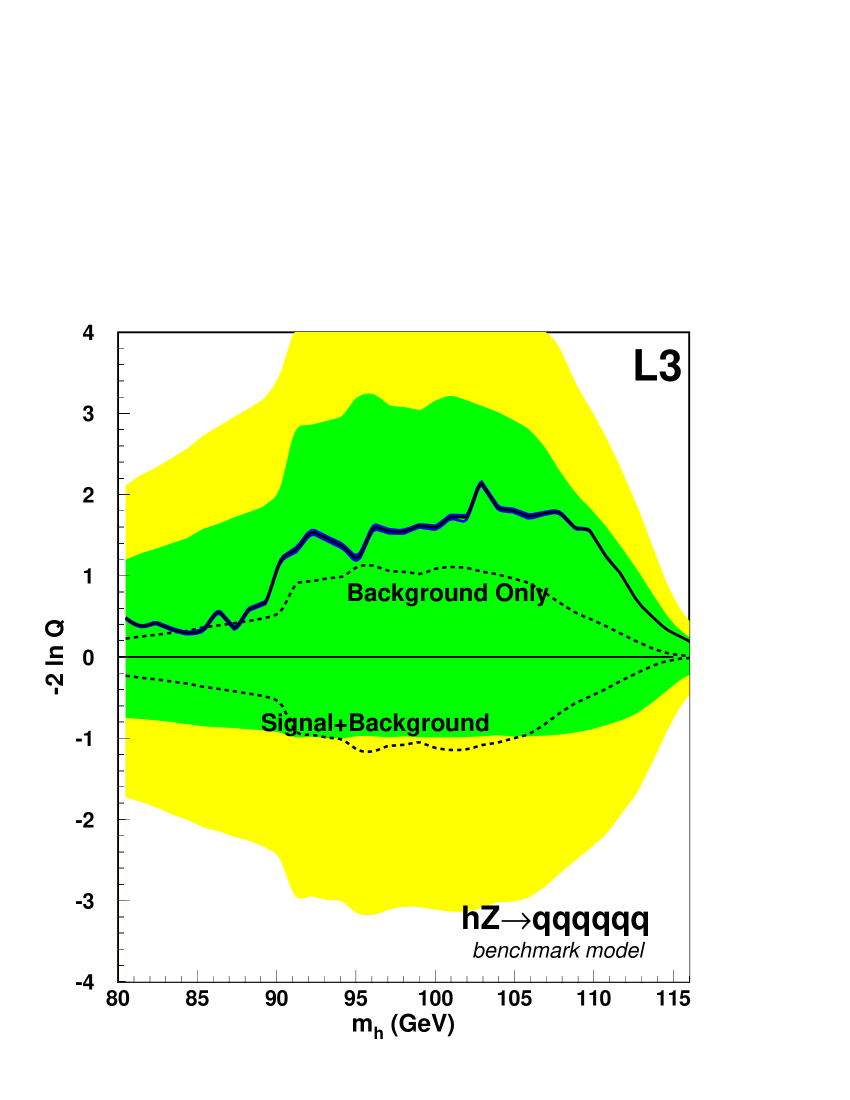
(c) Mass distribution of selected events	(d) $-2\ln Q$ curves for qqqqqq

Figure 4.4: Results for the $\textrm{hZ}\rightarrow\textrm{qqqqqq}$ search.

The $\textrm{qqqql}\nu$ channel has the highest total separation power of any of the channels. Its branching fraction is nearly as large as the qqqqqq branching fraction. The lepton and neutrino in the event improve the event identification and mass resolution. The observed $-2\ln Q$ curve lies within the $\pm 1\sigma$ region for most of the mass range, but the channel indicates an excess over the background-only prediction at masses above 110 GeV.

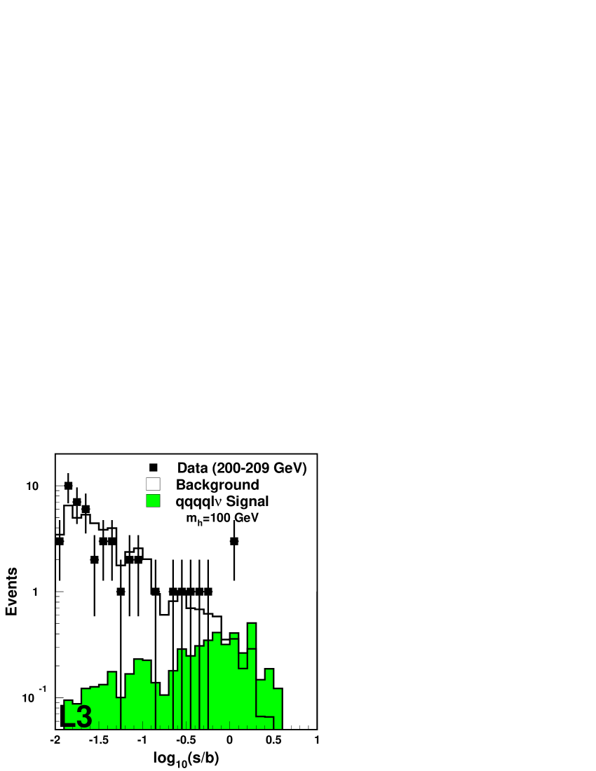
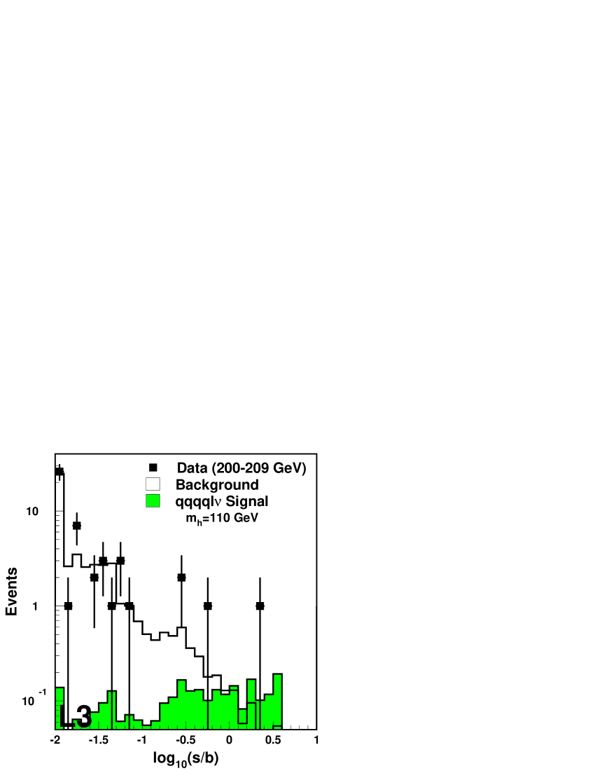
(a) Final variable rebinned in s/b for $m_{\textrm{h}}=100$ GeV	(b) Final variable rebinned in s/b for $m_{\textrm{h}}=110$ GeV
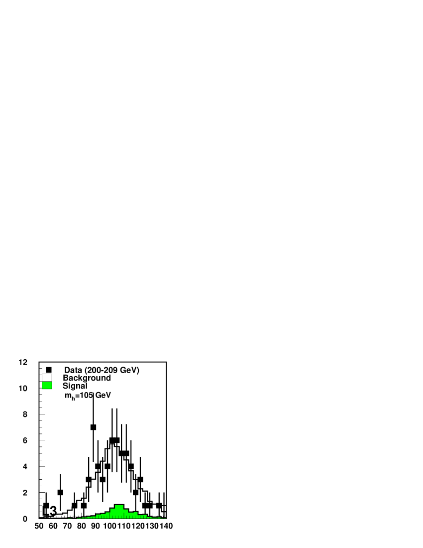
(c) Mass distribution of selected events	(d) $-2\ln Q$ curves

Figure 4.5: Results for the $\textrm{hZ}\rightarrow\textrm{qqqql}\nu$ search.

As shown in Figure 4.6d, the $\nu\nu\textrm{qqqq}$ channel is significantly deficit in data at masses below $m_{\scriptsize\mathrm{h}}$=90 GeV, where the W pair-production background dominates. At higher masses, the results closely follow the background-only expectation except for a candidate event near 100 GeV. The analysis is only effective for masses above $m_{\scriptsize\mathrm{Z}}$. The separation between the signal+background and background-only hypotheses for lower masses is quite small.

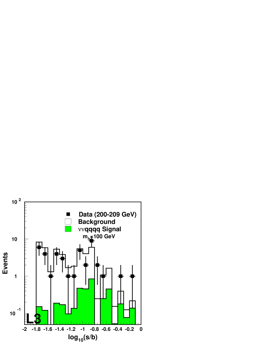
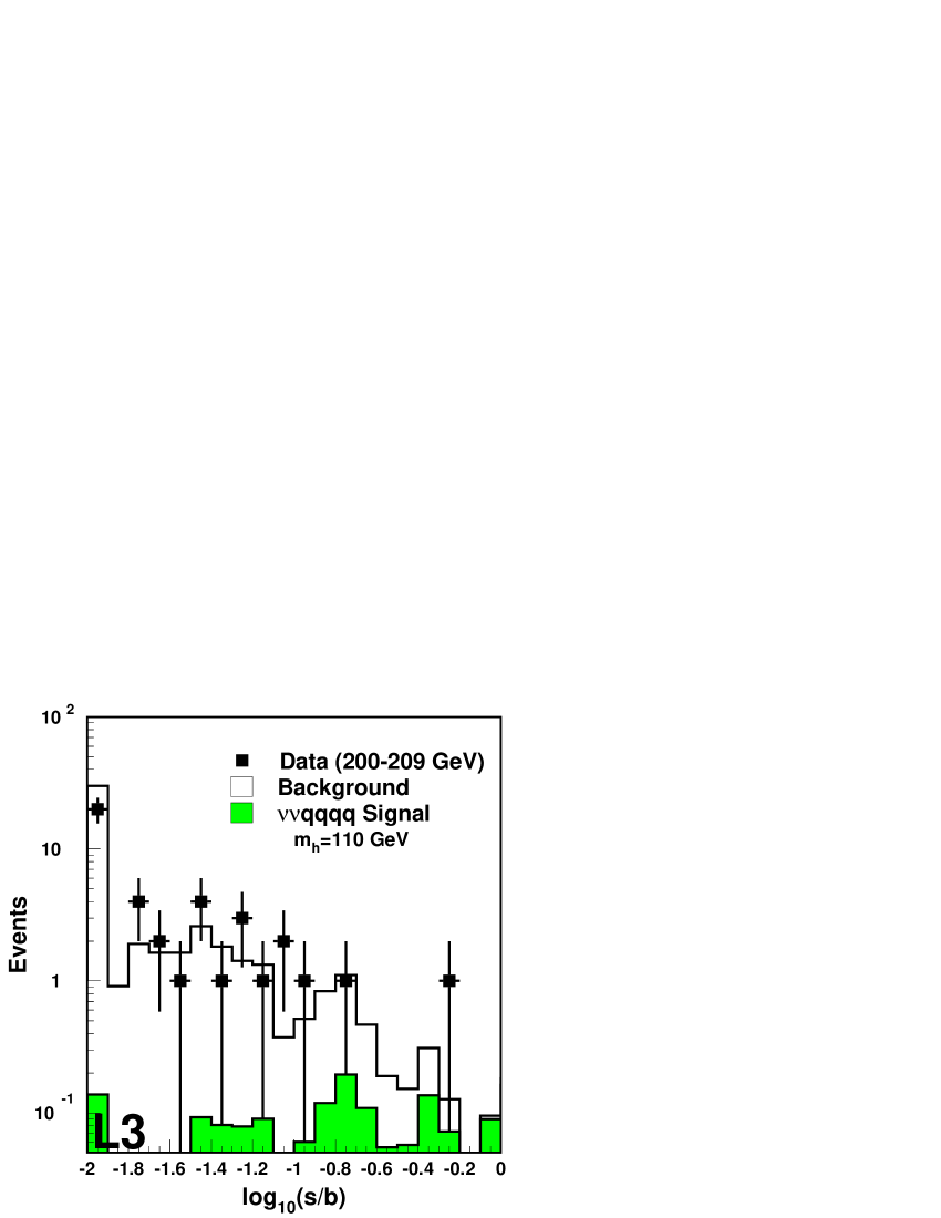
(a) Final variable rebinned in s/b for $m_{\textrm{h}}=100$ GeV	(b) Final variable rebinned in s/b for $m_{\textrm{h}}=110$ GeV
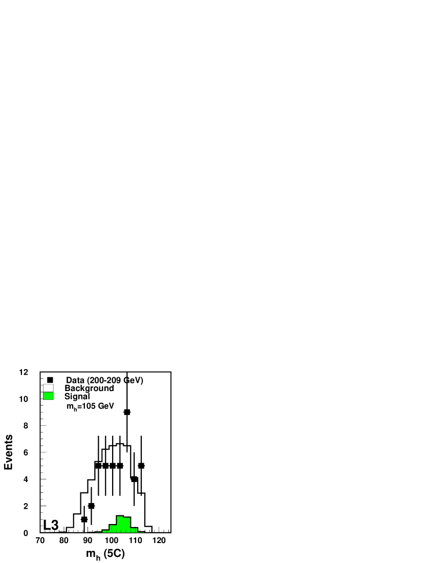
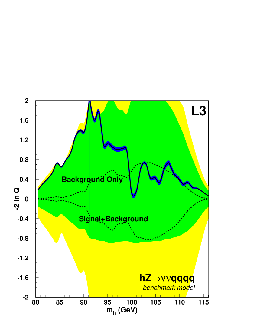
(c) Mass distribution of selected events	(d) $-2\ln Q$ curves

Figure 4.6: Results for the $\textrm{hZ}\rightarrow\nu\nu\textrm{qqqq}$ search.

The $\nu\nu\textrm{qql}\nu$ analysis has remarkably flat performance for lower masses, as shown in Figure 4.7c. Most channels suffer from low-mass backgrounds and the $\textrm{W}^{*}$ and $\textrm{W}^{(*)}$ becoming quite low-mass for $m_{\scriptsize\mathrm{h}}\simeq m_{\scriptsize\mathrm{Z}}$. The visible energy in $\nu\nu\textrm{qql}\nu$ is always small and the analysis is less sensitive to the masses of the Higgs decay bosons since they are hard to reconstruct at all. The observed results have a small constant excess for lower masses, increasing to a slightly larger excess for masses above 110 GeV. There is no mass plot for this channel, since the Higgs mass cannot be reconstructed.

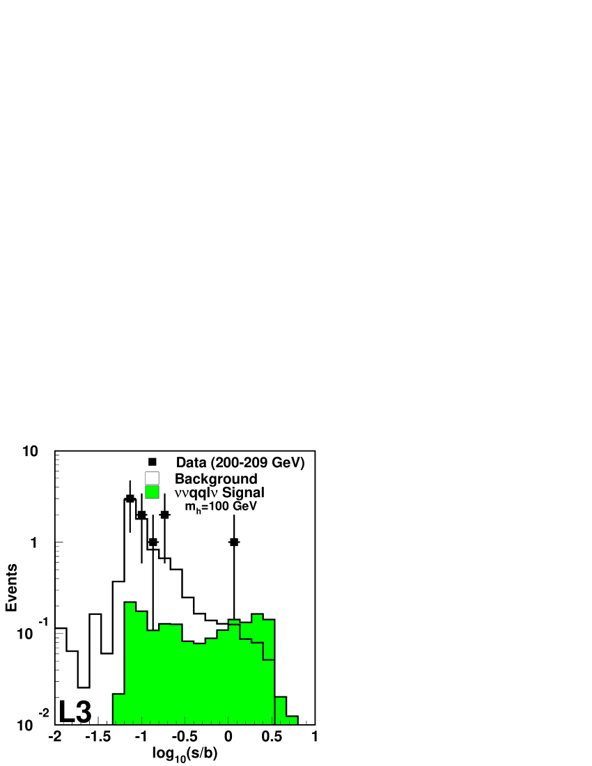
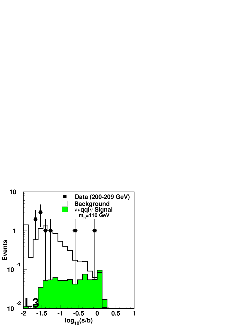
(a) Final variable rebinned in s/b for $m_{\textrm{h}}=100$ GeV	(b) Final variable rebinned in s/b for $m_{\textrm{h}}=110$ GeV
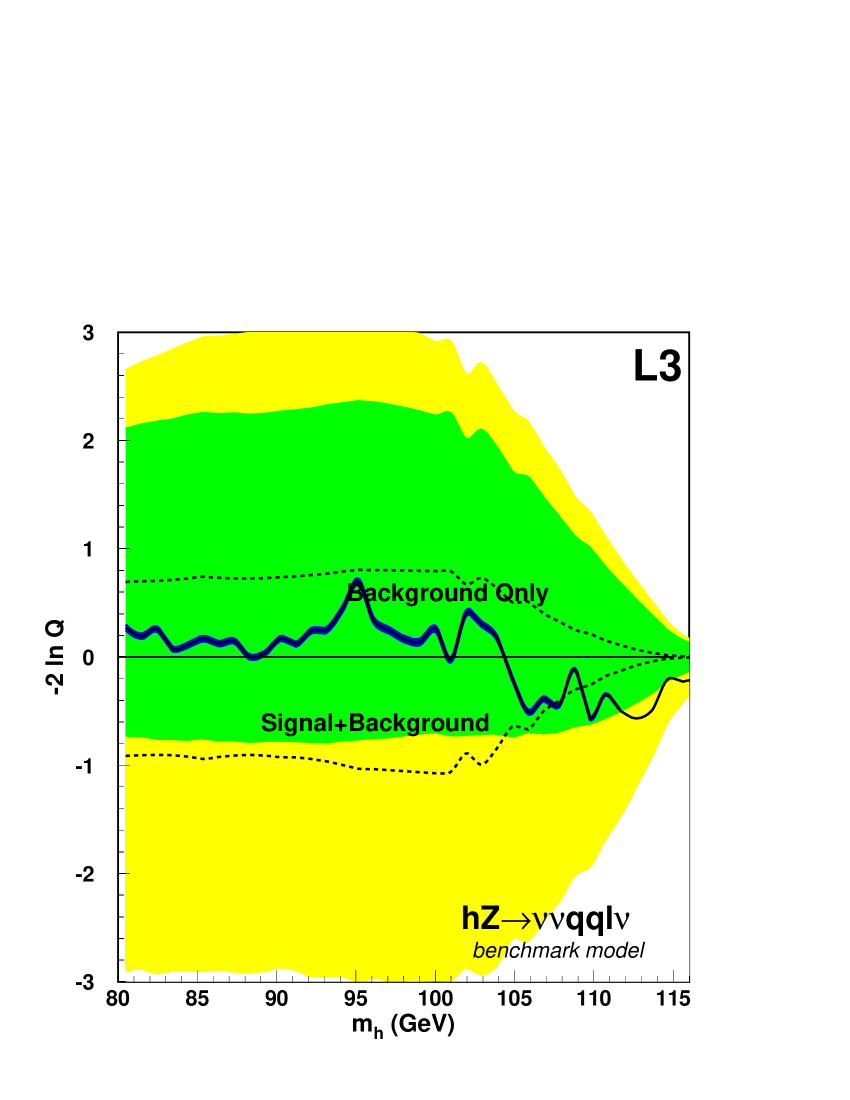
(c) $-2\ln Q$ curves

Figure 4.7: Results for the $\textrm{hZ}\rightarrow\nu\nu\textrm{qql}\nu$ search.

In the llqqqq channel, the effect of the ZZ background can be very clearly seen in 4.8d. The separation between background-only and signal+background has a pronounced narrowing near $m_{\scriptsize\mathrm{Z}}$. The channel selects a very small number of data events which makes the upper side of the $2\sigma$ band extremely narrow. The width is derived from a series of Poisson trials, and there are very few integer values available for a down-fluctuation from an observation of five events. The llqqqq channel is mildly deficit for small mass and high mass and matches the background-only expectation near and slightly above $m_{\scriptsize\mathrm{Z}}$.

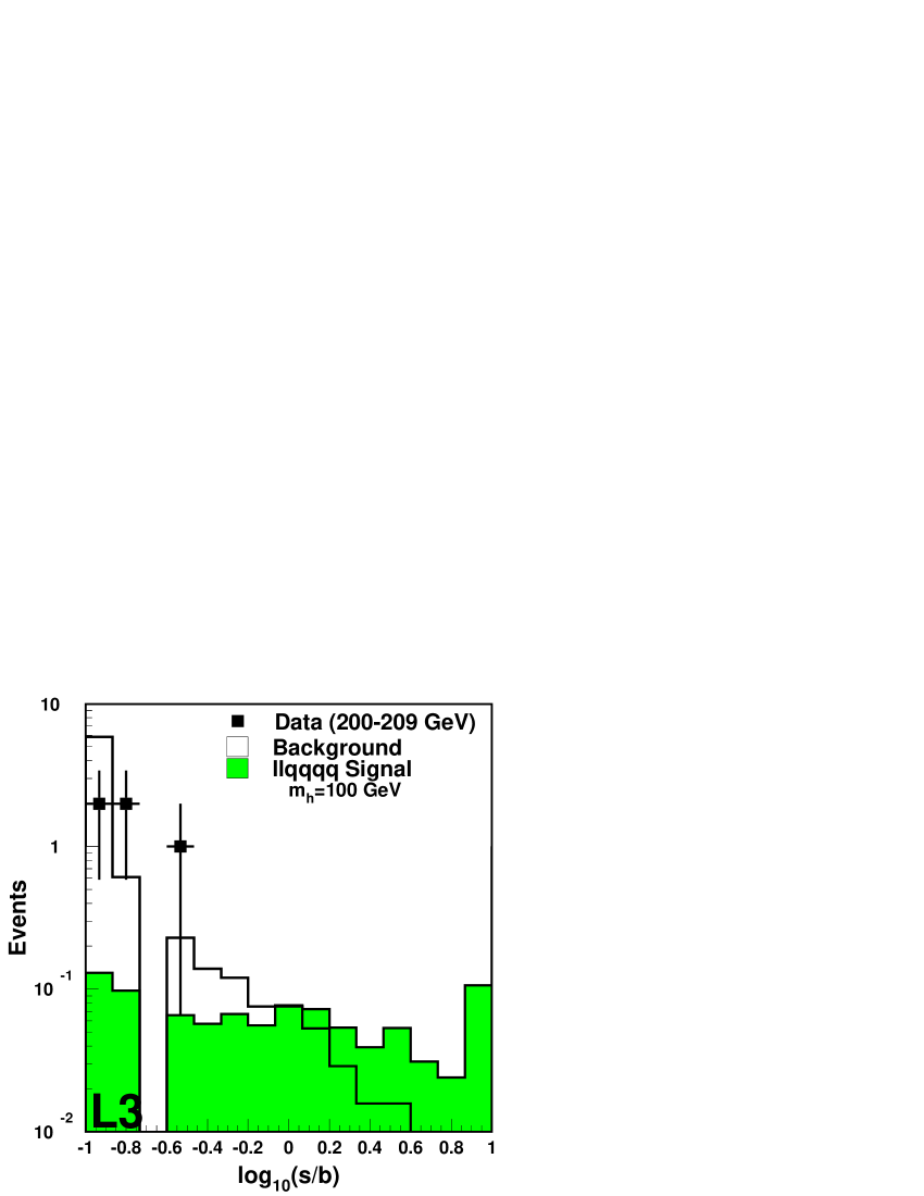
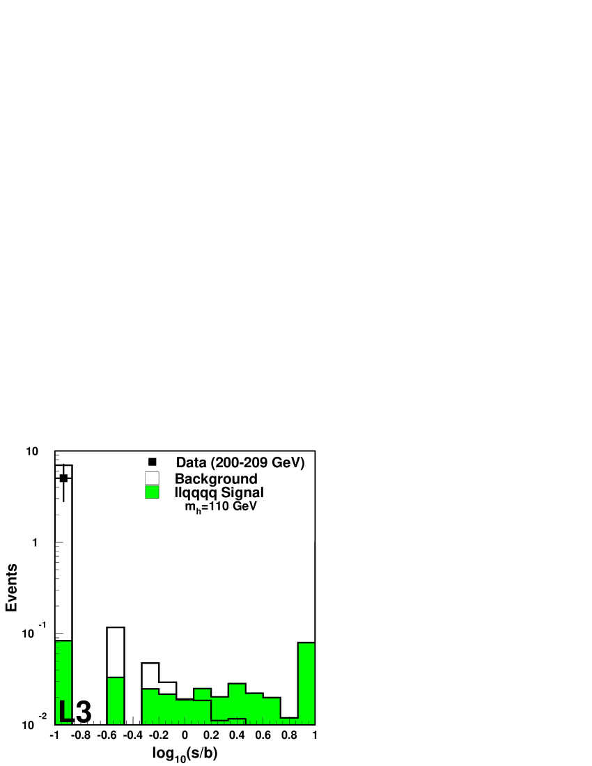
(a) Final variable rebinned in s/b for $m_{\textrm{h}}=100$ GeV	(b) Final variable rebinned in s/b for $m_{\textrm{h}}=110$ GeV
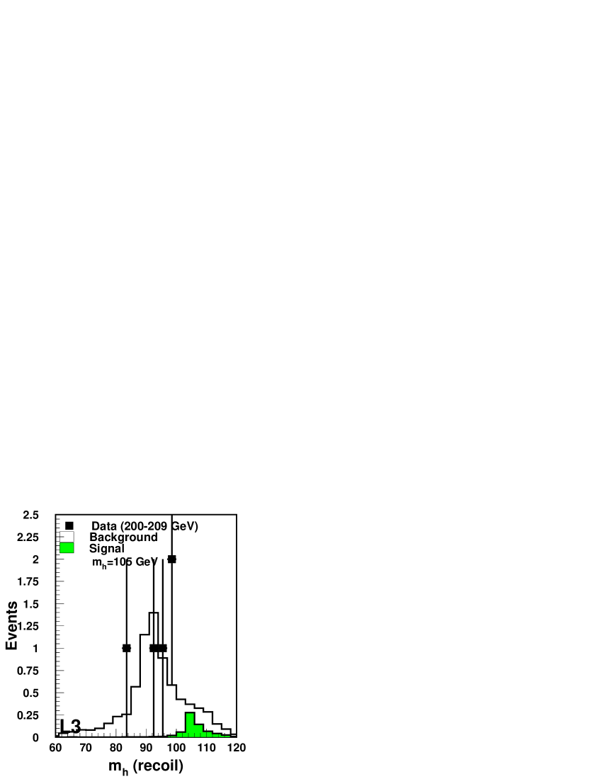
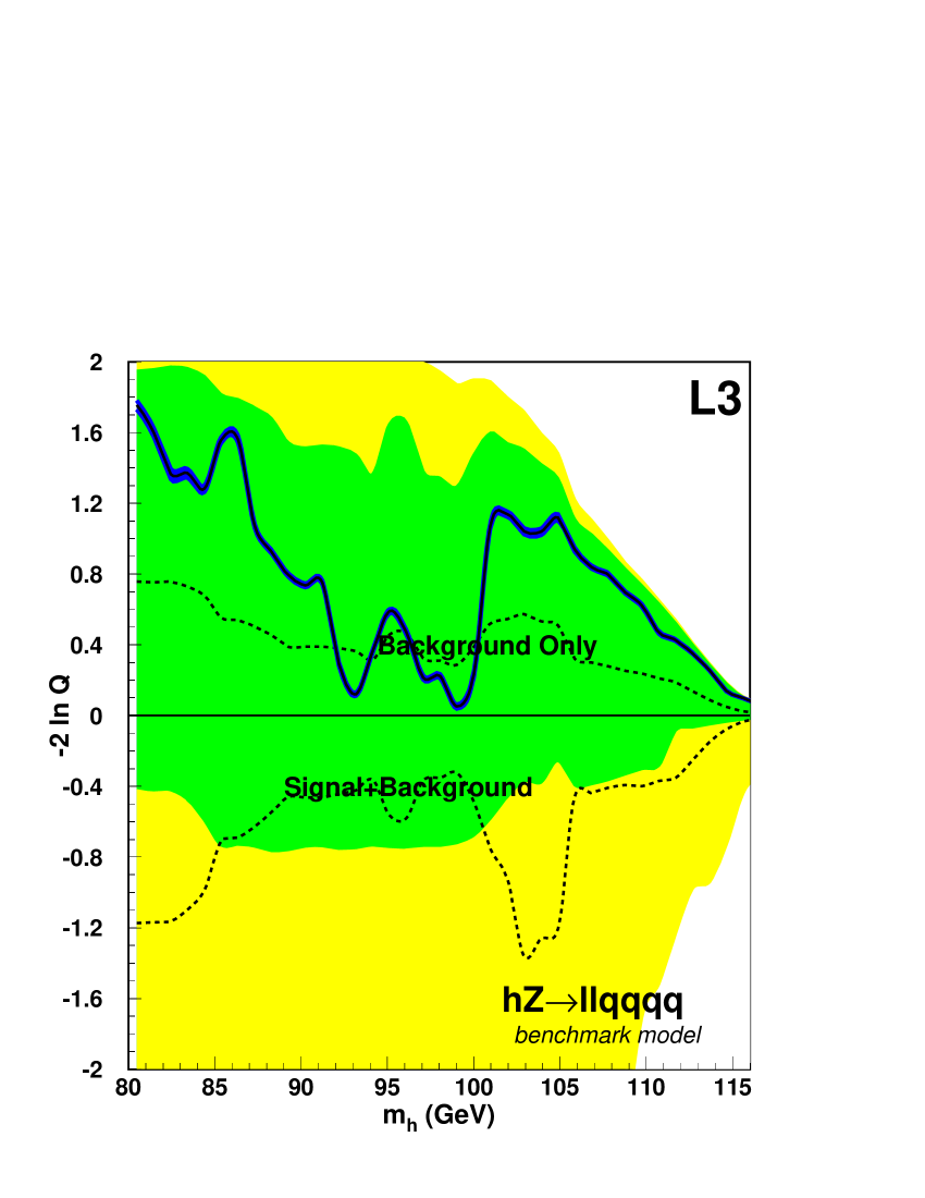
(c) Mass distribution of selected events	(d) $-2\ln Q$ curves

Figure 4.8: Results for the $\textrm{hZ}\rightarrow\textrm{llqqqq}$ search.

The $\textrm{qql}\nu\textrm{l}\nu$ channel has the smallest total search power of the analyzed channels, but it has some very high signal-to-background regions in the analysis. Figure 4.9d shows an excess at lower Higgs mass hypotheses, with a particular spike at 104 GeV. The analysis shows a small deficit for higher mass hypotheses.

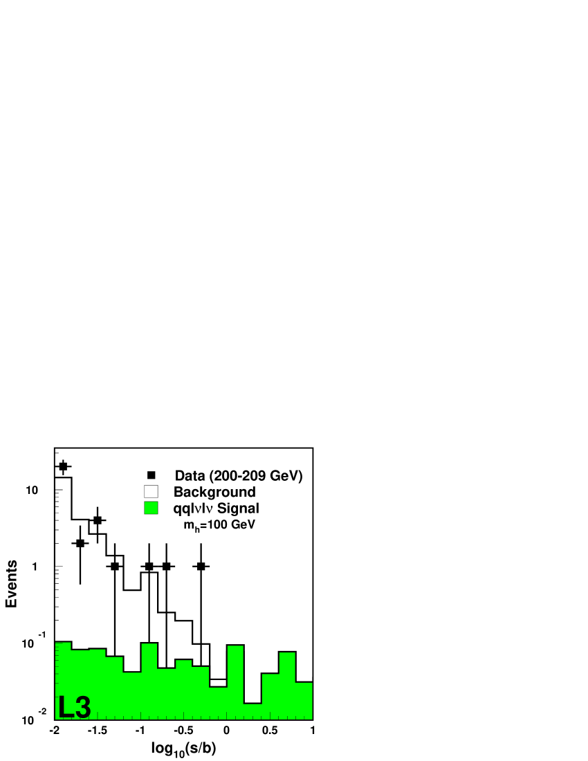
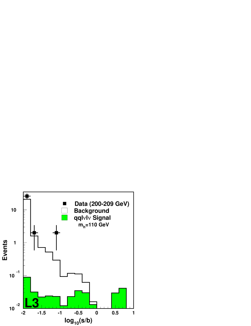
(a) Final variable rebinned in s/b for $m_{\textrm{h}}=100$ GeV	(b) Final variable rebinned in s/b for $m_{\textrm{h}}=110$ GeV
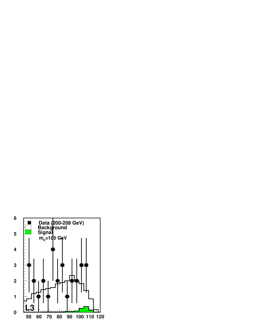
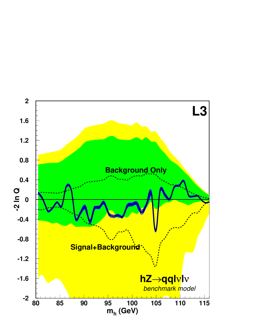
(c) Mass distribution of selected events	(d) $-2\ln Q$ curves

Figure 4.9: Results for the $\textrm{hZ}\rightarrow\textrm{qql}\nu\textrm{l}\nu$ search.

4.4.2 Combined $\textrm{h}\rightarrow\textrm{WW}/\textrm{ZZ}$ Results

The full search power of the analyses is obtained when all the analyses are combined together into a single analysis, as shown in Figure 4.10.

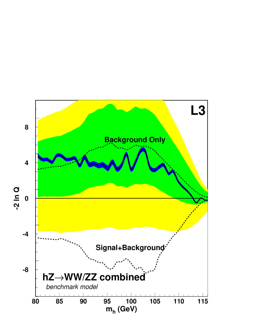
Figure 4.10: $-2\ln Q$ plot for the combined $\textrm{h}\rightarrow\textrm{WW}/ZZ$ search.

With all the channels combined, the $\textrm{h}\rightarrow\textrm{WW}/\textrm{ZZ}$ results can set limits on the production of a fermiophobic Higgs boson as a function of mass. Figure 4.11 shows the exclusion confidence levels under the benchmark fermiophobic model. The dashed line indicates the expected exclusion confidence level and the dark and light areas around the dashed line indicate the $\pm 1\sigma$ and $\pm 2\sigma$ expected regions respectively. The solid line indicates the observed exclusion confidence level, which exhibits the same deficit at low mass and slight excess at higher masses which is clear in the $-2\ln Q$ plot. Ignoring systematic errors, the observed exclusion region would be $83.7\textrm{ GeV }<m_{\scriptsize\mathrm{h}}<104.6\textrm{ GeV}$ with an unexcluded region between $88.9\textrm{ GeV}<m_{\scriptsize\mathrm{h}}<89.4\textrm{ GeV}$. The dotted lines around the solid curve indicate the effect of taking the systematic errors into account. The effect of the systematic errors is small : including errors, the exclusion region is $83.8\textrm{ GeV }<m_{\scriptsize\mathrm{h}}<104.2\textrm{ GeV}$ with an unexcluded region between $88.8\textrm{ GeV}<m_{\scriptsize\mathrm{h}}<89.6\textrm{ GeV}$.

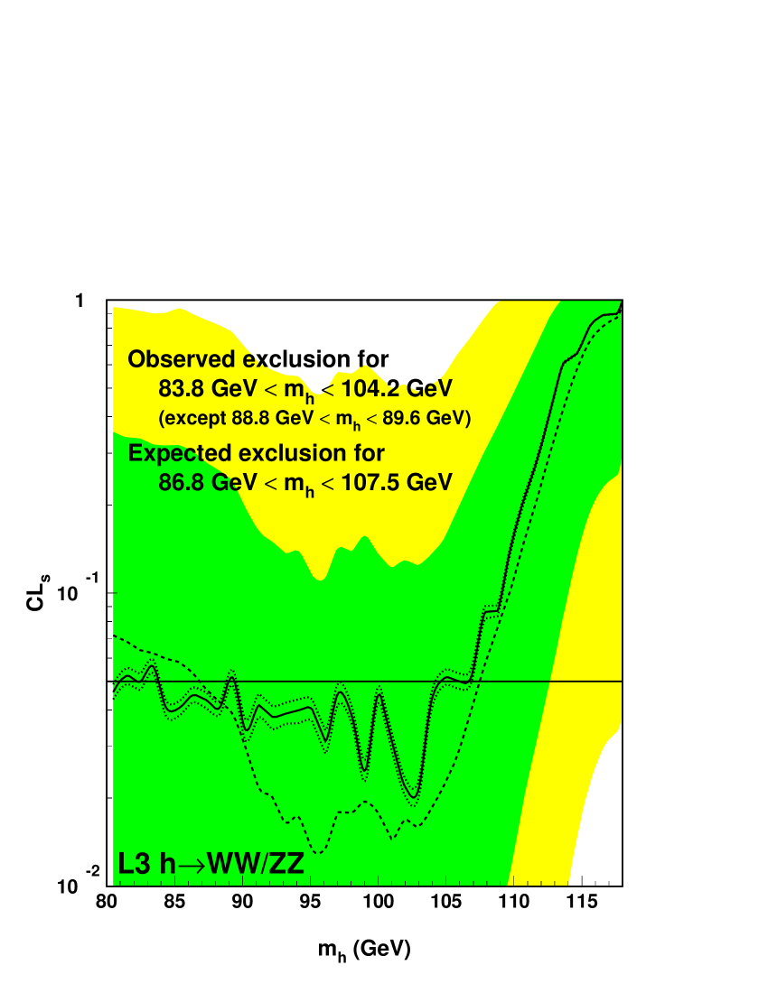
Figure 4.11: Confidence level limits in the benchmark fermiophobic model.

The dotted lines indicate the shifts from the observed confidence levels when systematic errors are taken into account.

Since the systematic errors are small, we neglect them for the more computationally difficult branching ratio limits.

As in the $\textrm{h}\rightarrow\gamma\gamma$ search, we obtain branching ratio limits by scaling the branching ratio to the value where the observed and expected confidence levels are 95%. This process produces the more model-independent result of Figure 4.12.

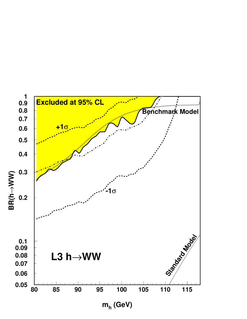
Figure 4.12: Branching ratio limits for the $\textrm{h}\rightarrow\textrm{WW}/\textrm{ZZ}$ search.

The predicted branching ratios of both the benchmark model and the Standard Model are given on the plot as dotted lines. The Standard Model $\textrm{H}\rightarrow\textrm{WW}$ branching ratio is too low by a factor of $\sim 30$ at 110 GeV for these analyses to exclude it, compared to a factor of $\sim 50$ for the LEP combined $\textrm{H}\rightarrow\gamma\gamma$ at the same mass.

4.5 Combined Fermiophobic Results

The results of the massive boson search can be combined with the LEP $\textrm{h}\rightarrow\gamma\gamma$ search results to give wider limits on fermiophobic models. For a single Higgs decay type, model-independent results can be derived by scaling the branching ratio of the Higgs to the given decay type as a function of mass to obtain a 95% CL limit. A general fermiophobic search with both $\textrm{h}\rightarrow\gamma\gamma$ and $\textrm{h}\rightarrow\textrm{VV}$ must consider both branching ratios separately as functions of the mass of the Higgs. A useful choice of parameterization is

$$\mathrm{Br}_{\scriptsize\mathrm{phobic}} = \textrm{BR}(\textrm{h}\rightarrow\gamma\gamma)+\textrm{BR}(\textrm{h}\rightarrow\textrm{WW})+\textrm{BR}(\textrm{h}\rightarrow\textrm{ZZ})$$

$$\mathrm{Br}_{\scriptsize\gamma\gamma} = \frac{\textrm{BR}(\textrm{h}\rightarrow\gamma\gamma)}{\mathrm{Br}_{\scriptsize\mathrm{phobic}}}.$$

Thus $\mathrm{Br}_{\scriptsize\gamma\gamma}$ represents the fraction of fermiophobic decays which are to $\gamma\gamma$ and can range from zero to one, while $\mathrm{Br}_{\scriptsize\mathrm{phobic}}$ represents the total Higgs branching fraction to pairs of gauge bosons. The search algorithm scans values of both $m_{\scriptsize\mathrm{h}}$ and $\mathrm{Br}_{\scriptsize\gamma\gamma}$ and determine the values of $\mathrm{Br}_{\scriptsize\mathrm{phobic}}$ for 95% CL expected and observed exclusion. The resulting plane is the most general result of the LEP fermiophobic search. The process is computationally intensive, since it involves millions of Monte Carlo trials for each scan point in the $40\times 40$ plane.

The results of the scan are plotted in Figure 4.13. The shades of gray indicate the value of $\mathrm{Br}_{\scriptsize\mathrm{phobic}}$ corresponding to an observed 95% confidence level. The dashed lines give the expected boundary locations for the color transitions. There is a an excess observed just above the Z mass independent of $\mathrm{Br}_{\scriptsize\gamma\gamma}$  which can be seen by the darker shades of color extending above the line which should be the color boundary. There are observed deficits for $\mathrm{Br}_{\scriptsize\gamma\gamma}>0.1$ in the low-mass region as well as the 97 GeV mass region. The line crossing the plot from upper left to lower right is the benchmark value of $\mathrm{Br}_{\scriptsize\gamma\gamma}$. The point where this line crosses the $\mathrm{Br}_{\scriptsize\mathrm{phobic}}=1.0$ gives the model-dependent limit. Using a fine-grained search, we obtain a limit of $m_{\scriptsize\mathrm{h}}$> 108.1 GeV with the expected limit of $m_{\scriptsize\mathrm{h}}$> 111.5 GeV, compared to $m_{\scriptsize\mathrm{h}}>106.5\textrm{ GeV}$ observed and $m_{\scriptsize\mathrm{h}}>109.6\textrm{ GeV}$ expected from the $\textrm{h}\rightarrow\gamma\gamma$ alone.

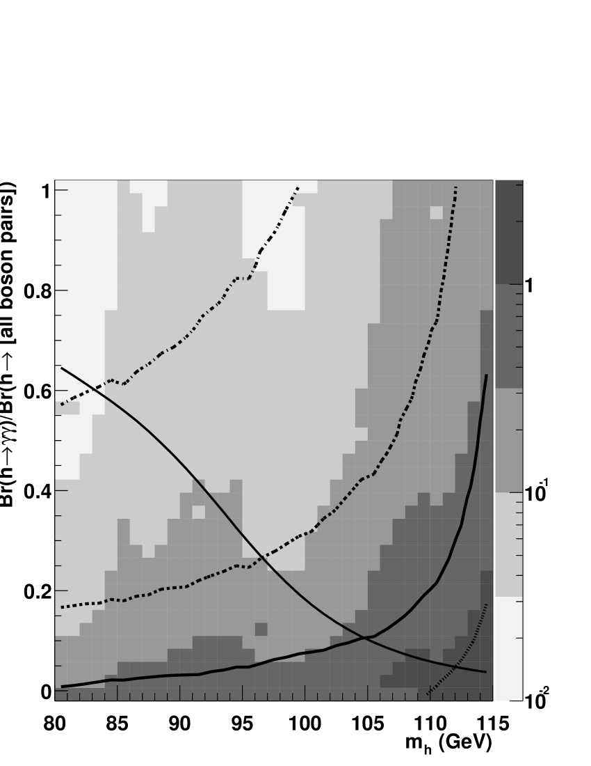
Figure 4.13: Results of the fermiophobic scan.

4.6 Conclusions

The first search for a Higgs boson decaying to massive vector bosons pairs has been remarkablely successful, though it did not discover the Higgs. The search established the first 95% confidence level limits for a Higgs decaying to massive vector boson pairs. Over the next decade, searches at the Tevatron, LHC, and a linear $\textrm{e}^{+}\textrm{e}^{-}$ collider will focus on the WW and ZZ channels for discovering and studying the Higgs [43], and this work should be a resource for these future studies.

Appendix A Final Variable Construction Techniques

Man is a tool-using animal. Without tools, he is nothing,
with tools he is all.

Thomas Carlyle

A.1 KEYS

The final Higgs search results are performed by comparing signal and background distributions. Choppiness will result in numerical difficulties for the limit-setting algorithm so these distributions need to be fairly smooth. However, the high performance of the Higgs search analyses means that very few Monte Carlo background events remain after selection to estimate the background. The solution adopted by the LEP Higgs Working Group is use the KEYS algorithm developed by Kyle Cranmer to smooth the final distributions.

The entire KEYS algorithm is fairly complicated and is fully described in [44], but the basic concept is straightforward. Each event is added to the distribution not as a spike at a given value, but as a Gaussian centered on that value. This technique, known as “kernel estimation,” is widely used. The key question is the width of the Gaussian used. KEYS calculates this width in two steps. First, it constructs an intermediate distribution using fixed widths dependent on the variance of the source data. Then, this intermediate distribution is used to determine the widths for the final smoothed result. Where the intermediate distribution is large, the Gaussians in the final distribution will be narrow. Where the intermediate distribution is small, the Gaussians will be wide. This process is shown in cartoon form in Figure A.1.

Figure A.1: The KEYS kernel-estimation smoothing process.

The actual value of each event in the distribution is given by the vertical lines. We replace each point by a Gaussian whose width depends on the density of points in the immediate neighborhood. Adding many Gaussians would make the distribution approach the dashed-line curve.

This technique is very effective at smoothing many distributions, including neural network distributions. In the case of neural network distributions where the distribution peaks at the edge and values above 1.0 and below 0.0 are not possible, we fold the Gaussians back across the y-axes.

In these analyses, we use our own implementation of the algorithm which uses a many-bin histogram rather than an event list for calculations. This modification greatly speeds the algorithm.

A.2 Neural Networks

In many analyses, there are multiple discriminating variables but usually only one variable can be used in the final fit or search. Traditionally, one applies hard cuts on all but one variables and uses the last as the “final variable”. In some circumstances, this technique limits the performance of the analysis since a simple cut does not extract all the distinguishing power available in a combination of the variables. One technique for combining variables is the neural network. The term “neural network” conjures up many images, but the networks used for analysis purposes are simply non-linear functions constructed in a certain manner with many parameters, where the parameters are determined in an iterative process from examples. There are many possible neural network structures and choices for combination and activation functions, but we will discuss only those used here and leave the general discussion to other texts [45].

Figure A.2: Diagram of a neural network.

This network has four input nodes, five hidden nodes, and one output node.

Consider a neural network as set of nodes, each with many inputs and one output. The output of the node can be connected to other nodes to construct a network, as in Figure A.2. The output of each node is a nonlinear function of its inputs. For the analysis networks, we form a weighted sum of all the inputs to the node and use the result as the argument of a sigmoid function to calculate the node output $O_{j}$:

$$O_{j}=\frac{1}{2}\left(\tanh(\sum_{i}w_{ij}I_{ij}+\beta_{j})+1\right),$$

where the $I_{ij}$ are the inputs to the $j$-th node and the $w_{ij}$ are the weights. Thus, for a network with $n$ inputs, a single hidden layer of $m$ nodes and a single output we can write the output as

$$O=\frac{1}{2}\left[\tanh\left(\sum^{m}_{i=1}w_{iO}\frac{1}{2}\left[\tanh(\sum^{n}_{j=1}w_{ji}I_{j}+\beta_{i})+1\right]+\beta_{O}\right)+1\right].$$

The only question is the determination of $w_{ij}$ and $\beta_{j}$ ; once these are set, a neural network is a straightforward function.

The weights used in the network are determined through a learning process. The network is first initialized with random weights. Then the trainer gives a pattern to the network and the network produces some output. The trainer then compares the desired output with the actual output and adjusts the weights by a small increment to make the output closer to the desired output, propogating the changes back through the network. The trainer repeats this process many times with different patterns until the network converges to a set of weights. There are several mathematical propogation techniques which have been developed for networks. We use the RPROP technique, which is somewhat faster than the classic backpropogation technique but otherwise similar [46]. All of our networks were trained using the Stuttgart Neural Network Simulator (SNNS) package [47]. SNNS features a batch training program and a conversion tool to make a trained network into simple and fast C code.

For high-energy physics use, we compose our patterns out of physically relevant variables using Monte Carlo signal and background to provide simulated patterns. Typically, the patterns specify that the network should output zero for background events and one for signal events. A fairly large number of patterns is required for training. The exact number required is dependent on the number of inputs, hidden nodes, and the level of corellation between inputs, but certainly more than 1000 events each of signal and background should be used if possible. During the training process, the training software presents each pattern in the set in random order and then the process repeats.

The training algorithm seeks to minimize the average error over all the patterns in the set, while the physics goal is generally to minimize the number of background events in the best signal region. In addition, a given pattern set will contain non-physical coorelations from sampling errors, so it is useful to check the performance of the network against a separate set which is not used for training. Between every second training cycle, we determine the network outputs for a test pattern set. From these, we determine the cut position which would leave 70% or 80% of the signal events. Then we count the number of background events which pass this cut. If this number has decreased from the last cycle, we save the network. Thus, the final network selected from the training is the network which has the lowest number of background events in the signal-pure region from the testing, rather than training set. This technique is somewhat complicated, but provides significantly better results than simply accepting the last network from the training.

A.3 Discriminant Final Variable

The neural network as described in Section A.2 is one way to combine multiple variables. However, training a network requires large numbers of signal events, which can obtained by combining many generated mass values together. This means that the mass itself cannot be used as a variable and some other technique is needed to include this important variable. The technique used in our analyses to combine such variables is to produce probability distributions of each of the final variables for each background type and signal mass hypothesis separately and combine them in a discriminant final variables for each event.

Let us take $s_{i}$ to be the probability distribution for variable $i$ for a given signal mass hypothesis, and $b^{j}_{i}$ to be the probability distribution for variable $i$ for background $j.$ We smooth these distributions using the modified version of the KEYS algorithm discussed above. If we consider the values of each variable for a given event as a vector $\overrightarrow{x}$ with components $x_{1},x_{2},\ldots$, then we form the quantity $p_{i}$ which represents probability that event with this value is signal as:

$$p_{i}=\frac{s_{i}(x_{i})}{s_{i}(x_{i})+\sum_{j}b^{j}_{i}(x_{i})}$$

for each variable $i$. Similarly, we can construct $q_{i}^{j}$ which represents the probability that an event with this value $x_{i}$ is of background type $j$:

$$q^{j}_{i}=\frac{b^{j}_{i}(x_{i})}{s_{i}(x_{i})+\sum_{k}b_{i}^{k}(x_{i})}.$$

We combine the values from each variable by multiplying, yielding the discriminant

$$f(\overrightarrow{x})=\frac{\prod_{i}p_{i}}{\prod_{i}p_{i}+\sum_{j}\prod_{i}q^{j}_{i}}.$$

The discriminant calculation may be more clear in the example in Figure A.3. Of course, in the actual calculation we use hundreds of bins to improve the smoothness of the distributions rather than the twenty of the example, but the principle is the same.

Figure A.3: Example of a two-variable discriminant calculation.

In this example, there are two variables. The background distribution is given by the empty curve and the signal distribution is given by the hatched curve. Consider an event with neural network ouput 0.82 and reconstructed mass of 108 GeV.

$$p_{1}=\frac{0.016}{0.016+0.097}=\frac{1.6}{11.3} p_{2}=\frac{0.036}{0.036+0.047}=\frac{3.6}{8.3}$$

$$q_{1}=\frac{0.097}{0.016+0.097}=\frac{9.7}{11.3} q_{2}=\frac{0.047}{0.036+0.047}=\frac{4.7}{8.3}$$

$$f=\frac{\frac{1.6}{11.3}\cdot\frac{3.6}{8.3}}{\frac{1.6}{11.3}\cdot\frac{3.6}{8.3}+\frac{9.7}{11.3}\cdot\frac{4.7}{8.3}}=\frac{5.76}{51.35}\approx 0.11$$

For a more signal-like event, $f$ would be closer to $1.0$, while for a very background-like event, $f\rightarrow 0.0$.

Appendix B Systematic Errors

The goal of systematic errors is quantify how much we don’t know about our data.

B.1 Strategy for Systematic Error Estimation

In the calculation of systematic errors, we want to determine what experimental or other processes might contribute to an error in our result. Given a reasonable estimate of the scale of these effects from inspection of large data and Monte Carlo samples, we determine how our results might be affected. The most important source of systematic errors is disagreements between the background Monte Carlo and data. A great deal of experimental effort each year was put into calibrating the detector and applying measured detector efficiencies to Monte Carlo. After applying these calibrations and measured efficiencies, the ensemble of events in the Monte Carlo match the actual conditions under which the data was taken as closely as possible. At the end of the process, disagreements between Monte Carlo and data may still occur, particularly in selected subsamples of the data.

We estimate the effect of possible shifts in the data using Monte Carlo. Such shifts are likely to be coorlated across variables. For example, one of the most important sources of systematic error is miscalibrations in the energy scale of the calorimeters. A shift in the energy scale would affect jet energies, visible energy, reconstructed masses, recoil masses, and many other quantities. To estimate the effect of an energy scale shift, we shift all the relavent variables at once in the approproriate directions for each event. We produce a set of final input files using the shifted events but keeping the probability density functions constant. We determine the shift in $\textrm{LLR}_{\textrm{b}}$ values compared to the unshifted inputs as a function of mass hypothesis. This process propogates the effect of uncertainities in physical quantities from the detector into the final results.

There are several other important sources of potential error besides the energy scale. Several analyses have significant dependency on the number of charged tracks overall and in jets. These analyses are sensitive to changes in the tracking efficiency. The lepton-containing analyses are sensitive to shifts in the variables used for lepton identification, but the use of smooth lepton quality variables makes the error reasonably well-behaved. Several analyses use event shape variables which depend mostly on cluster counting and can be a significant source of error since the largest known disagreement between L3 Monte Carlo and data is the number of clusters. Finally, there are errors due to the finite numbers of Monte Carlo events available for the analyses, particularly in the channels which are divided into six subchannels. We estimate this error by using the standard formula $\sqrt{\frac{\epsilon(1-\epsilon)}{N_{{\scriptsize\textrm{MC}}}}}$. We consider all errors of a given type to be corrolated between the channels and the center-of-mass energies except for Monte Carlo statistics.

B.2 Systematic Errors by Channel

Although we use the mass-hypothesis-dependent errors for the actual limit calculations, we give mass-averaged values of the systematic error coming from various sources in the tables below as a general guide to the relative importance of the different error sources in each channel.
qqqqqq Systematic Error Source Error Tracking Efficiency 2.1% Event Shape 1.2% Energy Scale 1.3% Monte Carlo Statistics 2% Total 3.4% $\textrm{qqqql}\nu$ Systematic Error Source Error Lepton Identification 3.8% Monte Carlo Statistics 3% Energy Scale 2.9% Tracking Efficiency 1.7% Total 5.9%
$\nu\nu\textrm{qqqq}$ Systematic Error Source Error Energy Scale 6.0% Event Shape 2.6% Monte Carlo Statistics 2% Tracking Efficiency 0.2% Total 6.8% $\nu\nu\textrm{qql}\nu$ Systematic Error Source Error Monte Carlo Statistics 4% Lepton Identification 2.8% Energy Scale 2.0% Tracking Efficiency 0.4% Total 5.3%
llqqqq Systematic Error Source Error Energy Scale 2.2% Tracking Efficiency 2.1% Monte Carlo Statistics 2% Lepton Identification 1.8% Total 4.1% $\textrm{qql}\nu\textrm{l}\nu$ Systematic Error Source Error Energy Scale 5.3% Lepton Identification 4.4% Tracking Efficiency 1.8% Monte Carlo Statistics 2% Total 7.4%

Thanks are due to Rene Brun et al. for a fine data analysis package, subject of course to the proviso: “PAW can do everything, but you cannot do anything with PAW.”

References

- [1] Stephen Myers. The LEP collider: from design to approval to commissioning. http://cern.web.cern.ch/CERN/Divisions/SL/history/lep_doc.html, November 1990.
- [2] Roger Bailey for the SL Division. Webpage: LEP operations in 2000. http://sl.web.cern.ch/SL/opnews/Lep/lep00.html, 2000.
- [3] B. Adeva et al. The construction of the L3 experiment. Nuclear Instruments and Methods in Physics Research A, 289:35–102, 1990.
- [4] A. Acciarri et al. T. Coan. The L3 silicon microvertex detector. Nuclear Instruments and Methods in Physics Research A, 351:300–312, 1994.
- [5] G. Basti et al. The L3 lead-scintillating fiber calorimeter. Nuclear Instruments and Methods in Physics Research A, 374:293–298, 1996.
- [6] L3 Collaboration. Higgs candidates in collisions at GeV. Physics Letters, B495:18–25, 2000.
- [7] A. et al. Adam. The forward muon detector of L3. Nuclear Instruments and Methods in Physics Research, Section A, 383:342, 1996.
- [8] R. Brun et al. Technical Report DD/EE/84-1, CERN, 1984. Revised 1987.
- [9] H. Fesefeldt. Technical Report PITHA 85/02, RWTH Aachen, 1985.
- [10] Torbjörn Sjöstrand. Computer Physics Communications, 82:74, 1994.
- [11] S. Jadach, B.F.L. Ward, and Z. Was. The precision monte carlo event generator KK for two-fermion final states in e+e- collisions. Computer Physics Communications, 130:260–325, 2000.
- [12] M. Skrzypek et al. Computer Physics Communications, 94:216, 1996.
- [13] F.A. Berends, R. Pittau, and R. Kleiss. Computer Physics Communications, 85:437, 1995.
- [14] R. Engel, J. Ranft, and S. Roesler. Physics Review, D 52:1459, 1995.
- [15] Sheldon L. Glashow. Nuclear Physics, 22:579, 1961.
- [16] Steven Weinberg. Physics Review Letters, 19:1264, 1967.
- [17] A. Salam. Weak and electromagnetic interactions. In N. Svartholm, editor, Elementary Particle Theory, page 367. Almqvist and Wiksell, Stockholm, 1968.
- [18] R. Brandelik et al. Evidence for planar events in e+ e- annihilation at high energies. Physics Letters B, 86B(2):243–9, 24 Sept. 1979.
- [19] G. Arnison et al. Experimental observation of isolated large transverse energy electrons with associated missing energy at =540 GeV. Physics Letters B, 122B(1):103–16, 24 Feb. 1983.
- [20] P. Bagnaia et al. Evidence for Z0 to e+ e- at the CERN pp collider. Physics Letters B, 129B(1-2):130–41, 15 Sept. 1983.
- [21] D.E. Groom et al. Review of particle physics. The European Physics Journal, C15:1, 2000.
- [22] Geraldus ’t Hooft and Marcus Veltman. Nuclear Physics, B44:189, 1972.
- [23] John F. Gunion, Howard E. Haber, Gordon Kane, and Sally Dawson. The Higgs Hunter’s Guide. Perseus Publishing, 1990.
- [24] Patrick Janot. The HZHA generator. In Physics at LEP2, volume CERN-96-01-V-2, pages 309–311, 1995.
- [25] H.P. Nilles. Phys. Rep., 110:1, 1984.
- [26] H.E. Haber and G.L. Kane. Phys. Rep., 117:75, 1985.
- [27] R. Barbieri. Riv. Nuovo Cim., 11(4):1, 1988.
- [28] R. Santos and A. Barroso. Renormalization of two-Higgs-doublet models. Physical Review D, 1997.
- [29] Juan Alcaraz and M.I. Josa. Signatures of fermiophobic higgses at LEP. Number 2740 in L3 Internal Notes.
- [30] LEP Electroweak Working Group. Combined preliminary data on Z parameters from the LEP experiments and constraints on the Standard Model. CERN/PPE, 94(187), November 1994.
- [31] CDF collaboration. Physical Review Letters, 74:2626, 1995.
- [32] D0 collaboration. Physical Review Letters, 74:2632, 1995.
- [33] Gerald Myatt for the Electroweak Working Group. Electroweak results and fits to the Standard Model. In Moriond 2002.
- [34] S. Bethke et al. Nuclear Physics B, 370:310, 1992.
- [35] Christopher G. Tully. Baryon Production in Z Decay. PhD thesis, Princeton University, 1997.
- [36] ALEPH Collaboration. Search for gamma-gamma decays of a Higgs boson produced in association with a fermion pair in collisions at LEP. Physical Letters B, 487:241–252, 2000.
- [37] DELPHI Collaboration. Search for a fermiophobic Higgs at LEP 2. Physics Letters B, 507:89, 2001.
- [38] L3 Collaboration. Search for a Higgs boson decaying into two photons in interactions at centre-of-mass energies up to 209 GeV. Physics Letters B, 2002.
- [39] OPAL Collaboration. Search for Higgs boson and other massive states decaying into two photons in collisions at 189 GeV. Physics Letters B, 464:311–322, 1999.
- [40] The OPAL Higgs Working Group. Searches for higgs bosons in extensions to the standard model in collisions at the highest LEP energies. OPAL Physics Note PN472, February 2001.
- [41] F. James, L. Lyons, and Y. Perrin, editors. 1st Workshop on Confidence Limits, number CERN-2000-005 in CERN Yellow Reports, 2000.
- [42] LEP Higgs WG. In LHWG Note 2001-08.
- [43] N. Kauer, T. Plehn, D. Rainwater, and D. Zeppenfeld. HWW as the discovery mode for a light Higgs boson. Physics Letters, B503:113–120, 2001.
- [44] Kyle Cranmer. Kernel estimation in high-energy physics. Computer Physics Communications, 2001.
- [45] Chris Bishop. Neural Networks for pattern recognition. Oxford University Press, 1995.
- [46] M. Riedmiller and H. Braun. A direct adaptive method for faster backpropogation learning: the RPROP algorithm. In Proceedings of the IEEE International Conference on Neural Networks, 1993.
- [47] University of Stuttgart, http://www-ra.informatik.uni-tuebingen.de/SNNS/. SNNS: Stuttgart Neural Network Simulator.