Dalitz Plot Analysis of the Decay $D^{+}\to K^{-}\pi^{+}\pi^{+}$ and Indication of
a Low-Mass Scalar $K\pi$ Resonance

Abstract

We study the Dalitz plot of the decay $D^{+}\to K^{-}\pi^{+}\pi^{+}$ with a sample of 15090 events from Fermilab experiment E791. Modeling the decay amplitude as the coherent sum of known $K\pi$ resonances and a uniform nonresonant term, we do not obtain an acceptable fit. If we allow the mass and width of the $K^{*}_{0}(1430)$ to float, we obtain values consistent with those from PDG but the $\chi^{2}$ per degree of freedom of the fit is still unsatisfactory. A good fit is found when we allow for the presence of an additional scalar resonance, with mass $797\pm 19\pm 43$ MeV/c² and width $410\pm 43\pm 87$ MeV/c². The mass and width of the $K^{*}_{0}(1430)$ become $1459\pm 7\pm 5$ MeV/c² and $175\pm 12\pm 12$ MeV/c², respectively. Our results provide new information on the scalar sector in hadron spectroscopy.

In this paper we present a Dalitz plot analysis of the Cabibbo-favored decay $D^{+}\to K^{-}\pi^{+}\pi^{+}$ using data from Fermilab experiment E791. Previous analyses of this decay e691-kpipi ; e687-kpipi modeled the amplitude as the coherent sum of known $K\pi$ resonances and a uniform non-resonant (NR) term. They observed that the NR term is strongly dominant, unlike other $D$ decays, and that the sum of the decay fractions substantially exceeds unity, indicating large interference. Moreover, the fits did not describe the Dalitz plot distributions well. In our analysis, we obtain similar results but with higher statistics. We study variations in the underlying model, including changes in form factors, tuning of resonance parameters, and the addition of known and new resonance structures. In particular, we investigate the scalar sector for which there has been much uncertainty for many years.

This study is based on the Fermilab E791 sample of $2\times 10^{10}$ events produced from interactions of a 500 GeV/c $\pi^{-}$ beam with five thin target foils (one platinum, four diamond). Descriptions of the detector, data set, reconstruction, and vertex resolutions can be found in Ref. ref791 . A clean sample of $K^{-}\pi^{+}\pi^{+}$ decays (charge-conjugate modes are implicit throughout this paper) was selected by requiring that the 3-prong decay (secondary) vertex be well-separated from the production (primary) vertex and located outside any solid material. The sum of the momentum vectors of the three tracks from the secondary vertex was required to point to the primary vertex, and each of the three tracks was required to pass closer to the secondary vertex than to the primary. We restricted the $p_{T}^{2}$ and $x_{F}$ ranges of the $D^{+}$ candidates to ensure an accurate model of our experiment in the Monte Carlo (MC) simulation. Finally, we required that the odd-charge track (track with charge opposite that of the $D^{\pm}$ candidate) from the secondary vertex be consistent with kaon identification in the Čerenkov counters cerenkov .

We fit the $K^{-}\pi^{+}\pi^{+}$ invariant mass distribution shown in Fig. 1(a) by the sum of $D^{+}$ signal and background terms. The signal was represented by the sum of two Gaussians, with parameters determined by the fit. We used MC simulations and data to determine both the shape and the size of charm backgrounds. The significant sources are reflections from $D_{s}^{+}\to K^{-}K^{+}\pi^{+}$ (via $\bar{K}^{*}K^{+}$ and $\phi\pi^{+}$), in which one kaon is misidentified as a pion. Other sources of charm background are either negligible or broadly distributed and thus safely included when we estimate combinatorial background, which was represented by an exponential function. The number of $D^{+}$ candidates obtained from the fit is $16190\pm 139$.

For the Dalitz plot analysis, we selected candidates in the $K\pi\pi$ mass range 1.85–1.89 GeV/c² (crosshatched region in Fig. 1(a)). This results in 15090 events, with about 6% due to background. Fig. 1(b) shows the corresponding Dalitz plot, $m^{2}_{12}$ vs. $m^{2}_{13}$, in which the kaon candidate is labeled particle 1, and the plot is symmetrized with respect to the two pions (particles 2, 3).

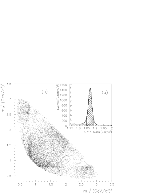
Figure 1: (a) The $K^{-}\pi^{+}\pi^{+}$ invariant mass spectrum. The shaded area corresponds to the background level. The crosshatched region is the sample used for the Dalitz plot analysis. (b) The $D^{+}\to K^{-}\pi^{+}\pi^{+}$ Dalitz plot, symmetrized for the indistinguishable pions.

To study the resonant structure in Fig. 1(b), an unbinned maximum likelihood fit is used. The likelihood ${\cal L}$ is computed as ${\cal L}=\prod_{\rm events}\left[\sum_{i=1}^{3}n_{B_{i}}{\cal P}_{B_{i}}+n_{S}{\cal P}_{S}\right]$, where ${\cal P}_{B_{i}}$ and ${\cal P}_{S}$ are the normalized probability density functions (PDF’s) for background and signal, respectively, and $n_{B_{i}}$ and $n_{S}$ are their fractional contributions. Each background PDF is written as ${\cal P}_{B_{i}}={1\over N_{B_{i}}}b_{i}(M){\cal F}_{B_{i}}(m^{2}_{12},m^{2}_{13})$, where $N_{B_{i}}$ is the normalization, $b_{i}(M)$ is the distribution in the $K\pi\pi$ mass spectrum, and ${\cal F}_{B_{i}}$ is the shape in the Dalitz plot. The shape of the combinatorial background is obtained from a fit to events above the signal peak in the $K\pi\pi$ mass range 1.92–1.96 GeV/c². The shapes of the $D_{s}^{+}\to\bar{K}^{*}K^{+}$ and $D_{s}^{+}\to\phi\pi^{+}$ backgrounds are from MC simulations.

The signal PDF is ${\cal P}_{S}={1\over N_{S}}g(M)\varepsilon(m^{2}_{12},m^{2}_{13})|{\cal A}|^{2}$, where $N_{S}$ is the normalization, $g(M)$ describes the signal shape in the $K\pi\pi$ mass spectrum, and $\varepsilon(m^{2}_{12},m^{2}_{13})$ is the acceptance across the Dalitz plot, including smearing. The signal amplitude $\cal A$ is a coherent sum of a uniform NR amplitude and resonant $K\pi$ amplitudes,

$${\cal A}=a_{0}e^{i\delta_{0}}{\cal A}_{0}+\sum_{n=1}^{N}a_{n}e^{i\delta_{n}}{\cal A}_{n}(m^{2}_{12},m^{2}_{13})\ ,$$ (1)

where each term is Bose symmetrized for the pions: ${\cal A}_{n}={\cal A}_{n}[({\bf 12}){\bf 3}]+{\cal A}_{n}[({\bf 13}){\bf 2}]$. The coefficients $a_{n}$ are magnitudes and the $\delta_{n}$ are relative phases.

Our first fit, referred to as Model A, includes only well-established resonances and fixes their masses and widths to PDG pdg values. This approach has been used in previous Dalitz-plot analyses (e.g., Refs. e687-kpipi ; argus ). The NR amplitude ${\cal A}_{0}$ is represented by a constant; i.e., it has no magnitude or phase variation across the Dalitz plot. Each resonant amplitude ${\cal A}_{n}$ ($n>0$) is written as ${\cal A}_{n}=\ BW_{n}~{}F_{D}^{(J)}~{}F_{n}^{(J)}~{}{\cal M}_{n}^{(J)}$. The $BW_{n}$ factor is the relativistic Breit-Wigner propagator, $BW_{n}=\{m^{2}_{n}-m^{2}-im_{n}\Gamma_{n}(m)\}^{-1}$, where $m$ is the invariant mass of the $K\pi$ pair forming a resonance (either $m_{12}$ or $m_{13}$), $m_{n}$ is the resonance mass, and $\Gamma_{n}(m)$ is the mass-dependent width. The factors $F_{D}^{(J)}$ and $F_{n}^{(J)}$ are Blatt-Weisskopf penetration factors blatt , which depend on the spin $J$ and the radii of the relevant mesons. In Model A, the radii are fixed as $r_{D}=5$ GeV^-1 for the $D$ meson and $r_{R}=1.5$ GeV^-1 for all $K\pi$ resonances argus . No form factors $F$ are used for scalar resonances. The term ${\cal M}_{n}^{(J)}$ accounts for the decay angular distribution. Ref. d3pi gives detailed expressions for all these functions; note that we use the opposite sign for the $BW_{n}$ term, for easier comparison of our results to those of Ref. e687-kpipi .

For Model A, we fix the NR parameters to be $a_{0}=1$ and $\delta_{0}=0$, and include all well-established $K\pi$ resonances; the only free parameters of the fit are the magnitudes $a_{n}$ and phases $\delta_{n}$ of the resonances. The so-called decay fraction for each mode is obtained by integrating its intensity (squared amplitude) over the Dalitz plot and dividing by the integrated intensity with all modes present. The fit results are listed in Table 1. We observe contributions from the same channels reported previously e691-kpipi ; e687-kpipi ; i.e., a high NR decay fraction (over 90%), followed by $\bar{K}^{*}_{0}(1430)\pi^{+}$, $\bar{K}^{*}(892)\pi^{+}$, and $\bar{K}^{*}(1680)\pi^{+}$. We also measure a small but statistically significant contribution from $\bar{K}^{*}_{2}(1430)\pi^{+}$. No other resonances considered are found to contribute. The sum of the decay fractions is $\sim 140\%$, indicating a high level of interference.

To assess the quality of the fit, we developed a fast-MC algorithm which produces binned Dalitz plot densities according to signal and background PDF’s, including detector efficiency and resolution. A $\chi^{2}$ is calculated from the difference between the binned Dalitz-plot-density distribution for data and that for fast-MC events generated using the parameters obtained from the fit of Model A. The $\chi^{2}$ summed over all bins is 167 for 63 degrees of freedom ($\nu$). The largest contributions to this $\chi^{2}$ come from bins at low $K\pi$ mass. In Fig. 2(a) we show the mass-squared projections; the top (bottom) plot shows the lower (higher) mass combination. The points represent data and the solid line represents fast-MC simulation of Model A. The main discrepancies occur below 0.6 (GeV/c²)² and around 2.5 (GeV/c²)². These discrepancies, and the large value of $\chi^{2}/\nu$, motivated us to study alternative ways to model the decay amplitude.

Table 1: Results of the Dalitz plot fits. Models A and B are without $\kappa$; Model C is with $\kappa$. For each mode the first row lists the decay fraction in percent, the second row lists the magnitude of the amplitude ($a_{n}$), and the third row lists the relative phase ($\delta_{n}$). The first error listed is statistical, and the second error (when listed) is systematic.

Mode	Model A	Model B	Model C
NR	$90.9\pm 2.6$	$89.5\pm 16.1$	$13.0\pm 5.8\pm 4.4$
	$1.0$ (fixed)	$2.72\pm 0.55$	$1.03\pm 0.30\pm 0.16$
	$0^{\circ}$(fixed)	$(-49\pm 3)^{\circ}$	$(-11\pm 14\pm 8)^{\circ}$
	–	–	$47.8\pm 12.1\pm 5.3$
$\kappa\pi^{+}$	–	–	$1.97\pm 0.35\pm 0.11$
	–	–	$(187\pm 8\pm 18)^{\circ}$
	$13.8\pm 0.5$	$12.1\pm 3.3$	$12.3\pm 1.0\pm 0.9$
$\bar{K}^{*}(892)\pi^{+}$	$0.39\pm 0.01$	1.0 (fixed)	$1.0$ (fixed)
	$(54\pm 2)^{\circ}$	$0^{\circ}$ (fixed)	$0^{\circ}$ (fixed)
	$30.6\pm 1.6$	$28.7\pm 10.2$	$12.5\pm 1.4\pm 0.5$
$\bar{K}^{*}_{0}(1430)\pi^{+}$	$0.58\pm 0.01$	$1.54\pm 0.75$	$1.01\pm 0.10\pm 0.08$
	$(54\pm 2)^{\circ}$	$(6\pm 12)^{\circ}$	$(48\pm 7\pm 10)^{\circ}$
	$0.4\pm 0.1$	$0.5\pm 0.3$	$0.5\pm 0.1\pm 0.2$
$\bar{K}^{*}_{2}(1430)\pi^{+}$	$0.07\pm 0.01$	$0.21\pm 0.18$	$0.20\pm 0.05\pm 0.04$
	$(33\pm 8)^{\circ}$	$(-3\pm 26)^{\circ}$	$(-54\pm 8\pm 7)^{\circ}$
	$3.2\pm 0.3$	$3.7\pm 1.9$	$2.5\pm 0.7\pm 0.3$
$\bar{K}^{*}(1680)\pi^{+}$	$0.19\pm 0.01$	$0.56\pm 0.48$	$0.45\pm 0.16\pm 0.02$
	$(66\pm 3)^{\circ}$	$(36\pm 25)^{\circ}$	$(28\pm 13\pm 15)^{\circ}$
$\chi^{2}/\nu$	167/63	126/63	46/63

For our second fit, Model B, we allow the mass and width of the scalar $K^{*}_{0}(1430)$ resonance to float. In addition, we include form factors to account for the finite size of the decaying mesons in this scalar transition torn ; cleotau . The amplitude is written as $F^{(0)}_{D}F^{(0)}_{n}BW_{n}$, in which the form factors are Gaussian: $F^{(0)}=\exp(-p^{*}{}^{2}/(2k_{0}^{2}))$. The factor $p^{*}$ is the momentum of the decay products, $k_{0}=\sqrt{6}/r$, and $r$ is the decaying meson radius. These radii ($r_{D}$ and $r_{R}$ introduced above) become additional free parameters in the fit. The results of this fit are listed in the middle column of Table 1. The decay fractions obtained are very similar to those found for Model A, but the $\chi^{2}/\nu$ is improved, dropping from 167/63 to 126/63. The mass and width of the $K^{*}_{0}(1430)$ obtained by the fit are $1416\pm 27$ MeV/c² and $250\pm 21$ MeV/c² respectively, which are close to the PDG values of $1412\pm 6$ MeV/c² and $294\pm 23$ MeV/c² pdg . The meson radii obtained are $r_{D}=0.8\pm 1.0$ GeV^-1 and $r_{R}=1.8\pm~{}3.4$ GeV^-1.

Since Model B still does not give a satisfactory fit, we allow for an additional scalar amplitude (Model C). For this extra amplitude, we use Gaussian form factors similar to those used for the $K^{*}_{0}(1430)$ thresh . The decay fractions and relative phases obtained by the fit are listed in the right-most column of Table 1. In the table we denote the additional scalar resonance as “$\kappa$”. In fact, discussions of the existence of such a resonance are found in the literature kapparef1 ; nokapparef . The fit results are very different from those obtained for Models A and B, the NR decay fraction drops from 90% to $(13\pm 6)$%; the $\kappa\pi^{+}$ channel is dominant with a decay fraction of $(48\pm 12)$; and the sum of all fractions is $\sim 90\%$, with smaller interference effects. The $\chi^{2}/\nu$ decreases to 46/63, substantially lower than those for Models A and B. For the $K_{0}^{*}(1430)$ resonance, we measure $m_{K_{0}^{*}(1430)}=1459\pm 7\pm 12$ MeV/c² and $\Gamma_{K_{0}^{*}(1430)}=175\pm 12\pm 12$ MeV/c². These values are significantly higher and narrower, respectively, than those given by the PDG pdg which are taken from LASS lass . See also dunwoodie . The mass and width of the additional resonance ($\kappa$) are $797\pm 19\pm 43$ MeV/c² and $410\pm 43\pm 87$ MeV/c², respectively. The meson radii obtained in Model C are $r_{D}=5.0\pm 0.5$ GeV^-1 and $r_{R}=1.6\pm 1.3$ GeV^-1. The $K\pi$ mass-squared projections are shown in Fig. 2(b).

Figure 2: $m^{2}(K\pi)_{\rm low}$ and $m^{2}(K\pi)_{\rm high}$ projections for data (error bars) and fast MC (solid line): Models A (a) and C (b).

To better understand our results for Model C, we perform the following test. For Models B and C we use the fast-MC to generate an ensemble of 1000 “experiments,” with each experiment having a sample size Poisson-distributed around our observed sample size. For each experiment we calculate $\Delta w_{B,C}\equiv-2({\rm ln}\,{\cal L}_{B}-{\rm ln}\,{\cal L}_{C})$, where ${\cal L}_{B}$ and ${\cal L}_{C}$ are the likelihood functions evaluated with parameters from Models B and C, respectively. For the ensemble generated without $\kappa\pi^{+}$, $\langle\Delta w_{B,C}\rangle=-123$; i.e., Model B has greater likelihood. For the ensemble generated with $\kappa\pi^{+}$, $\langle\Delta w_{B,C}\rangle=143$; i.e., Model C has greater likelihood. In both cases the rms of the distributions is about 23. For the data, $\Delta w_{B,C}=123$. This value is similar to that obtained for fast-MC events generated according to Model C, and it is very different from that of events generated according to Model B.

We investigate the stability of our results and estimate systematic errors from the following studies. We divide the total sample into disjoint subsamples according to $D$ charge, bins of $p_{T}^{2}$, $x_{F}$, and $K\pi\pi$ invariant mass, and repeat the analysis. We perform fit variations by changing fixed parameters of the fit: background parameterizations, and the mass and width of the $K^{*}(1680)$. We also repeat the analysis for samples selected with tighter and looser event selection criteria. These studies lead to the systematic errors quoted in the text and Table 1. The mass obtained for the $\kappa$, and the mass and width obtained for the $K^{*}_{0}(1430)$, are found to vary relatively little; e.g., $m_{\kappa}$ varies in the range 770–860 MeV/$c^{2}$. The width of the $\kappa$, and the $\kappa\pi^{+}$ and NR decay fractions, are found to vary much more: $\Gamma_{\kappa}$ ranges from 298–543 MeV/$c^{2}$ and the decay fractions range from 28–63% and 31–5%, respectively. The largest NR fraction obtained (31%) remains substantially lower than that obtained without a $\kappa$ resonance.

We have also studied the stability of our results with respect to the theoretical model. For example, we modified the $\kappa$ Breit-Wigner to have a “running mass” term as proposed by Törnqvist torn . We varied the momentum dependence of the $\kappa$ form factors. We introduced Gaussian form factors for all other resonant states. We varied the shape of the NR term. In all cases we obtained similar results for the $\kappa$ mass and width within errors; however, the details of the parameterizations affect the relative $\kappa\pi^{+}$ and NR contributions by up to a factor of two.

Finally, we have checked whether other models without a scalar $\kappa$ provide acceptable fits. We tried a toy model (T) by replacing the $\kappa$ complex Breit-Wigner by a Breit-Wigner amplitude with no phase variation. This model converged to a similar mass and width ($871\pm 10$ MeV/c² and $427\pm 23$ MeV/c², respectively) but with large decay fractions for this extra amplitude and for the NR amplitude, reflecting strong interference. The fast-MC gave $\langle\Delta w_{T,C}\rangle=60$ (rms of 16) for an ensemble generated according to Model C, and $\langle\Delta w_{T,C}\rangle=-60$ for an ensemble generated with toy model parameters. For the data, $\Delta w_{T,C}=45$; i.e., the data prefers that the additional amplitude have a phase variation and not just a larger amplitude at low $K\pi$ mass. We also replaced the scalar $\kappa$ resonance by vector and tensor resonances to test the angular distribution. The vector resonance model (V) converged to mass and width values of $1103\pm 45$ MeV/$c^{2}$ and $350\pm 93$ MeV/$c^{2}$, respectively, with a decay fraction of only 1.8% and a large NR fraction. The fast-MC gave $\langle\Delta w_{V,C}\rangle=140$ (rms of 23) for the ensemble generated according to Model C, and $\langle\Delta w_{V,C}\rangle=-140$ for the ensemble generated with vector parameters. For the data, $\Delta w_{V,C}=116$; i.e., the data prefers that the additional resonance be scalar rather than vector. We were not able to make the tensor model converge, the width being driven to large negative values. We also performed a variety of fits to study the NR shape bediaga in variants of Model A, i.e., without an additional scalar amplitude. We fitted the NR amplitude to polynomials, and we also allowed for different interfering angular distributions, but none of these fits were as good as that of Model C.

In summary, we have performed a Dalitz plot analysis of the decay $D^{+}\to K^{-}\pi^{+}\pi^{+}$. We compared models in which the signal amplitude ${\cal A}$ is the coherent sum of a uniform NR term and Breit-Wigner $K\pi$ resonances. Our best fit is obtained when we include an additional scalar resonance with a phase variation corresponding to that of a Breit-Wigner; this state subsequently accounts for about half of the decay rate. The mass and width obtained are $797\pm 19\pm 43$ MeV/c² and $410\pm 43\pm 87$ MeV/c², respectively. The fit mass and width of the $K^{*}_{0}(1430)$ depend on whether this additional Breit-Wigner is included or not. When not included, $m_{K^{*}(1430)}=1416\pm 27$ MeV/c² and $\Gamma_{K^{*}(1430)}=250\pm 21$ MeV/c² (statistical errors only), in agreement with PDG values pdg . When included, $m_{K^{*}(1430)}=1459\pm 7\pm 5$ MeV/c² and $\Gamma_{K^{*}(1430)}=175\pm 12\pm 12$ MeV/c². Overall we conclude that the scalar contribution to ${\cal A}$ is not adequately described by the sum of a uniform non-resonant term and a $K^{*}_{0}(1430)$ term. Including an additional scalar resonance in ${\cal A}$ results in a good fit to the data while the mass and the width of the $K^{*}_{0}(1430)$ appear higher and narrower, respectively, than previous reported results.

We thank E. van Beveren and N. Törnqvist for useful discussions. We gratefully acknowledge the assistance of the staffs of Fermilab and of all the participating institutions. This research was supported by CNPq (Brazil), CONACyT (Mexico), FAPEMIG (Brazil), the Israeli Academy of Sciences and Humanities, PEDECIBA (Uruguay), the U.S. Department of Energy, the U.S.-Israel Binational Science Foundation, and the U.S. National Science Foundation.

References

- [1] E691 Collaboration, J.C. Anjos et al., Phys. Rev. D 48, 56 (1993).
- [2] E687 Collaboration, P.L. Frabetti et al., Phys. Lett. B 331, 217 (1994).
- [3] J.A. Appel, Ann. Rev. Nucl. Part. Sci. 42, 367 (1992); D. Summers et al., hep-ex/0009015; S. Amato et al., Nucl. Instrum. Methods A 324, 535 (1993); E.M. Aitala et al., Eur. Phys. J. direct C 4, 1 (1999).
- [4] D. Bartlett et al., Nucl. Instrum. Methods A 260, 55 (1987).
- [5] D.E. Groom et al., Eur. Phys. Jour. C 15, 1 (2000).
- [6] ARGUS Collaboration, H. Albrecht et al., Phys. Lett. B 308, 435(1993); CLEO Collaboration, S. Kopp et al., Phys. Rev. D 63, 092001 (2001).
- [7] J.M. Blatt and V.F. Weisskopf, Theoretical Nuclear Physics, John Wiley & Sons, New York, 1952.
- [8] E791 Collaboration, E.M. Aitala et al., Phys. Rev. Lett. 86, 770 (2001).
- [9] N.A. Törnqvist, Z. Phys. C 68, 647 (1995).
- [10] CLEO Collaboration, D.M. Asner et al., Phys. Rev. D 61, 012002 (2000).
- [11] There remains the question about how best to characterize broad states near threshold. This subject is considered in Ref. [9], and also recently by E. van Beveren and G. Rupp, Eur. Phys. J. C 22, 493 (2001).
- [12] E. van Beveren et al., Z. Phys. C 30, 615 (1986); S. Ishida et al., Prog. Theor. Phys. 98, 621 (1997); D. Black et al., Phys. Rev. D 58, 054012 (1998); J.A. Oller et al., Phys. Rev. D 59 074001 (1999); M. Jamin et al., Nucl. Phys. B587, 331 (2000); C.M. Shakin and H. Wang, Phys. Rev. D 63, 014019 (2001); R. Delbourgo and M.D. Scadron, Int. J. Mod. Phys. A 13, 657 (1998); M. Ishida, Prog. Theor. Phys. 101, 661 (1999); J.A. Oller and E. Oset, Phys. Rev. D 60, 074023 (1999); F.E. Close and N.A. Törnqvist, hep-ph/0204205 (2002).
- [13] A.V. Anisovich and A.V. Sarantsev, Phys. Lett. B 413, 137 (1997); S.N. Cherry and M.R. Pennington, Nucl. Phys. A688, 823 (2001); N.A. Törnqvist and A.D. Polosa, in Heavy Quarks at Fixed Target, edited by I. Bediaga, J. Miranda, and A. Reis, Frascati Physics Series, Vol. XX (Laboratori Nazionali di Frascati, Roma, Italy, 2000), p. 385.
- [14] LASS Collaboration, D. Aston et al., Nucl. Phys. B296, 493 (1988).
- [15] A new fit to the LASS data for the S–wave scattering amplitude in the elastic range (up to threshold) yields MeV/c2 and MeV/c2. Private communication from W.M. Dunwoodie for the LASS Collaboration.
- [16] I. Bediaga, C. Göbel, and R. Méndez-Galain, Phys. Rev. Lett. 78, 22 (1997) and Phys. Rev. D 56, 4268 (1997).