The BABAR Collaboration

A sample of about 5500 $\kern 1.79993pt\overline{\kern-1.79993ptB}{}^{0}\rightarrow{D^{*}}^{+}\rho^{-}$ and 700 ${\kern 1.79993pt\overline{\kern-1.79993ptB}{}^{0}\rightarrow{D^{*}}^{+}a_{1}^{-}}$ events is identified, using the technique of partial reconstruction, among 22.7 million $B\kern 1.79993pt\overline{\kern-1.79993ptB}{}$ pairs collected by the BABAR experiment at the PEP-II storage ring. With these events, the $B^{0}$ lifetime is measured to be $1.616\pm 0.064\pm 0.075$ ps. This measurement serves as validation for the procedures required to measure $\sin(2\beta+\gamma)$ with partial reconstruction of $\kern 1.79993pt\overline{\kern-1.79993ptB}{}^{0}\rightarrow{D^{*}}^{+}\rho^{-}$.

1 Introduction

The neutral $B$ meson decay modes $B\rightarrow{D^{*}}^{+}h^{-}$, where $h^{-}$ is a light hadron ($\pi^{-},\rho^{-},a_{1}^{-}$), have been proposed [1] for use in theoretically clean measurements of the Cabibbo-Kobayashi-Maskawa [2] unitarity triangle parameter $\sin(2\beta+\gamma)$. Since the time-dependent CP asymmetries in these modes are expected to be of order 2%, large data samples and multiple decay channels are required for a statistically significant measurement. The low efficiency of reconstructing the $D^{0}$ produced in the ${D^{*}}$ decay leads to significant loss of signal events. Partial reconstruction of the $B$ meson results in substantially larger efficiency, albeit with higher backgrounds. The overall $\sin(2\beta+\gamma)$ sensitivity is expected to be roughly similar for partial and full reconstruction, and about 90% of the partially reconstructed events cannot be fully reconstructed. Therefore, both full and partial reconstruction can and should be used for the $\sin(2\beta+\gamma)$ measurement.

The measurement of the $B^{0}$ lifetime, presented here, constitutes a first step toward measuring $\sin(2\beta+\gamma)$ with partial reconstruction of $\kern 1.79993pt\overline{\kern-1.79993ptB}{}^{0}\rightarrow{D^{*}}^{+}\rho^{-}$. In this analysis, we have developed the procedures for candidate reconstruction, background characterization, vertexing, and fitting, all critical components of the time-dependent $\sin(2\beta+\gamma)$ analysis.

2 The BABAR Detector and Data Sample

The data used in this analysis were collected with the BABAR detector at the PEP-II storage ring. The data consist of 22.7 million $B\kern 1.79993pt\overline{\kern-1.79993ptB}{}$ pairs, corresponding to an integrated luminosity of 20.7 $\mbox{\,fb}^{-1}$ recorded at the $\mathchar 28935\relax{(4S)}$ resonance. In addition, 2.6 $\mbox{\,fb}^{-1}$ were collected about 40 MeV below the resonance. This off-resonance sample is used to study the continuum, $e^{+}e^{-}\rightarrow q\overline{q}$ background, where $q=\{u,d,s,c\}$.

The BABAR detector, described in detail elsewhere [3], consists of five sub-detectors. Surrounding the beam-pipe is a five-layer silicon vertex tracker (SVT), providing precision measurements of the positions of charged particles close to the interaction point and tracking of charged particles with low transverse momentum. Outside the support tube that surrounds the SVT is a 40-layer drift chamber (DCH), filled with an 80:20 helium-isobutane gas mixture. The DCH provides charged particle momentum measurements in a 1.5 T magnetic field, and ionization energy loss measurements that contribute to charged particle identification. Surrounding the DCH is a detector of internally reflected Cherenkov light (DIRC), providing charged particle identification. Outside the DIRC is a CsI(Tl) electromagnetic calorimeter (EMC), used mainly to detect and measure the energy of photons and to provide electron identification. The EMC is surrounded by a superconducting coil, which generates the magnetic field for tracking. Outside the coil, the flux return iron is instrumented with resistive plate chambers, used mainly for muon identification.

PEP-II is an asymmetric energy storage ring, with positron and electron beam energies of about 3.11 and 9.0 GeV. The center-of-mass (CM) frame of the average $e^{+}e^{-}$ collision is therefore boosted along the $z$ direction in the lab frame, enabling time-dependent measurements involving reconstruction of $B$ mesons.

3 Analysis Method

3.1 Partial Reconstruction

To partially reconstruct a $\kern 1.79993pt\overline{\kern-1.79993ptB}{}^{0}\rightarrow{D^{*}}^{+}\rho^{-}$ candidate , only the $\rho$ and the $\pi_{s}$, the soft pion from the decay ${D^{*}}^{+}\rightarrow D^{0}\pi_{s}^{+}$ decay, are reconstructed. The angle between the momenta of the $B$ and the $\rho$ in the CM frame is then computed:

$$\cos\theta_{B\rho}={M_{{D^{*}}^{+}}^{2}-M_{B^{0}}^{2}-M_{\rho}^{2}+E_{\rm CM}E_{\rho}\over 2P_{B}|\vec{p}_{\rho}|},$$ (1)

where $M_{x}$ is the mass of particle $x$, $E_{\rho}$ and $\vec{p}_{\rho}$ are the measured CM energy and momentum of the $\rho$, $E_{\rm CM}$ is the total CM energy of the beams, and $P_{B}=\sqrt{E_{\rm CM}^{2}/4-M_{B^{0}}^{2}}$. Given $\cos\theta_{B\rho}$ and the measured four-momenta of the $\pi_{s}$ and the $\rho$, the $B$ four-momentum may be calculated up to an unknown azimuthal angle $\phi$ around ${\vec{p}}_{\rho}$. For every a value of $\phi$, the expected $D$ four-momentum, ${\cal P}_{D}(\phi)$, is determined from four-momentum conservation, and the $\phi$-dependent “missing mass” is calculated, $m(\phi)\equiv\sqrt{|{\cal P}_{D}(\phi)|^{2}}$. With $m_{\rm max}$ and $m_{\rm min}$ being the maximum and minimum values of $m(\phi)$ obtained by varying $\phi$, we define the missing mass, $m_{\rm miss}\equiv{1\over 2}\left[m_{\rm max}+m_{\rm min}\right]$. This variable peaks around $M_{D^{0}}$, the nominal $D^{0}$ mass, for signal events, with a spread of about 3.5 MeV, while background events are more broadly distributed.

We define the $D^{*}$ helicity angle $\theta_{D^{*}}$ to be the angle between the directions of the $D$ and the $B$ in the $D^{*}$ rest frame. The value of $\cos\theta_{D^{*}}$ is computed as in Ref. [4]. The $\rho$ helicity angle $\theta_{\rho}$ is defined as the angle between the directions of the $\pi^{0}$ (from the decay of the $\rho$) and the CM frame in the $\rho$ rest frame. Since the $\kern 1.79993pt\overline{\kern-1.79993ptB}{}^{0}\rightarrow{D^{*}}^{+}\rho^{-}$ decay is $(87.8\pm 4.5)\%$ longitudinally polarized [5], the $\cos\theta_{\rho}$ and $\cos\theta_{D^{*}}$ distributions of signal events peak toward $\pm 1$. Background events have fairly flat distributions, with $B\kern 1.79993pt\overline{\kern-1.79993ptB}{}$ background increasing in the region of soft $\pi_{s}$ and $\pi^{0}$, making $\cos\theta_{D^{*}}$ and $\cos\theta_{\rho}$ useful for background suppression. With knowledge of $\cos\theta_{D^{*}}$ and $\cos\theta_{B\rho}$, the 3-momentum of the $D$ is determined, up to a two-fold ambiguity and detector resolution effects.

3.2 Event Selection

In order to suppress the continuum background, we select events in which the ratio of the 2nd to the 0th Fox-Wolfram coefficients [6] is smaller than 0.35. Charged $\rho$ candidates are identified by their decay to a “hard” charged pion, $\pi_{h}$, and a $\pi^{0}$. To suppress fake $\pi^{0}$ candidates, the $\pi^{0}$ momentum in the CM frame is required to be greater than 400 MeV. The invariant mass of the $\pi^{0}$ candidate must be within 20 MeV of the nominal $\pi^{0}$ mass. Both the $\pi_{h}$ and $\pi_{s}$ candidate tracks are required to originate within 1.5 cm of the interaction point in the $x-y$ plane (the plane perpendicular to the beam) and within $\pm 10$ cm of the interaction point along the direction of the beams. Tracks are rejected if their specific ionization and/or Cherenkov angle indicate that they are highly likely to be a kaon or a lepton. The invariant mass $m(\rho)$ of the $\rho$ candidate must be between 0.45 and 1.1 GeV.

The computed cosine of the angle between the $B$ and $\rho$ must satisfy $|\cos\theta_{B\rho}|\leq 1$. To suppress combinatoric background, we require $|\cos\theta_{\rho}|>0.3$ and $|\cos\theta_{D^{*}}|>0.3$, and reject events in the range $\cos\theta_{\rho}>0.3$ and $\cos\theta_{D^{*}}<-0.3$.

For each $\rho^{\pm}\pi_{s}^{\mp}$ pair that satisfies the above requirements, $m_{\rm miss}$ is calculated. The pair with the smallest value of $|m_{\rm miss}-M_{D^{0}}|$ in the event is selected, and all others are discarded. Similarly, the “wrong-sign” $\rho^{\pm}\pi_{s}^{\pm}$ pair with the smallest $|m_{\rm miss}-M_{D^{0}}|$ is retained for background studies, as described below. Right-sign events in the range $1.810<m_{\rm miss}<1.840$ GeV are classified as sideband events, and are used for background studies. Right- and wrong-sign events satisfying $m_{\rm miss}>1.845$ GeV are classified as signal region events. All other events are discarded. The efficiency of signal events to satisfy all the signal region criteria is 6.4%.

Events that could be fully reconstructed in the $D^{0}$ decay modes $D^{0}\rightarrow K^{-}\pi^{+}$ or $K^{-}\pi^{+}\pi^{0}$ are tagged as fully reconstructed. In addition to satisfying the partial reconstruction criteria above, fully reconstructed events are identified by requiring that the reconstructed $D$ invariant mass be within 40 MeV of $M_{D^{0}}$, the difference between the $D^{*}$ and $D$ invariant masses be between 142 and 150 MeV, the reconstructed CM $B$ energy be within 50 MeV of $E_{\rm CM}/2$, and $\mbox{$m_{\rm ES}$}>5.25$ GeV, where $\mbox{$m_{\rm ES}$}\equiv\sqrt{E_{\rm CM}^{2}/4-p_{B}^{2}}$ is the beam energy substituted mass and $p_{B}$ is the reconstructed CM momentum of the $B$ meson.

3.3 Measurement of the Decay Time Difference

The decay position $z_{\rm rec}$ of the partially reconstructed $B$ candidate along the beam direction is determined by constraining the $\pi_{h}$ track to originate from the beam-spot in the $x-y$ plane. To account for the $B$ meson flight in the $x-y$ plane, $30~{}\mu{\rm m}$ are added in quadrature to the beam-spot size. The $\pi_{s}$ is not used in this vertex fit in order to simplify the classification of the background, and since its contribution to the vertex precision is small, due to multiple scattering.

The decay position $z_{\rm other}$ of the other $B$ meson along the beam direction, is obtained with all tracks excluding the $\pi_{h}$, the $\pi_{s}$, and any track whose CM angle with respect to either of the two calculated directions of the $D$ is smaller than 1 radian. This “cone cut” reduces $N^{D}_{\rm tr}$, the number of $D$ daughter tracks used in the other $B$ vertex. The remaining tracks are fit with a constraint to the beam-spot in the $x-y$ plane. The track with the largest contribution to the $\chi^{2}$ of the vertex, if greater than 6, is removed from the vertex, and the fit is carried out again, until no track fails this requirement.

The decay time difference $\Delta t=(z_{\rm rec}-z_{\rm other})/\gamma\beta c$ is then calculated, where $\gamma\beta$ is the CM frame boost. The value of $\gamma\beta$ is continuously determined from the beam energies, and averages 0.55. The estimated error $\sigma_{{}_{\Delta t}}$ in the measurement of $\Delta t$ is calculated from the parameters of the tracks used in the two vertex fits.

Events are rejected if the $\chi^{2}$ probability of the $\pi_{h}$ vertex fit is smaller than 1%, or if the $\chi^{2}$ probability of the other $B$ vertex is smaller than 0.5%. We also require $|\Delta t|<15$ ps and $0.3<\sigma_{{}_{\Delta t}}<4$ ps.

The quantities $z_{\rm rec}$ and $z_{\rm other}$ are computed in the same way for fully reconstructed candidates as they are for partially reconstructed candidates. Using the Monte Carlo simulation, it is verified that with the 1 radian cone cut, the $N^{D}_{\rm tr}$ distribution of events that are fully reconstructed in the mode $D^{0}\rightarrow K^{-}\pi^{+}$ or $K^{-}\pi^{+}\pi^{0}$ is in good agreement with the distribution of partially reconstructed events.

3.4 Backgrounds

The types of events in the partially reconstructed on-resonance sample are classified as follows:

1. Signal: $\kern 1.79993pt\overline{\kern-1.79993ptB}{}^{0}\rightarrow{D^{*}}^{+}\rho^{-}$ events, in which the $\pi_{h}$ is correctly identified. This requirement ensures that $z_{\rm rec}$ is the decay position of the $B$ meson, up to the effect of detector resolution. The $\pi_{s}$ or the $\pi^{0}$ candidates may be mis-reconstructed.

2. ${\kern 1.79993pt\overline{\kern-1.79993ptB}{}^{0}\rightarrow{D^{*}}^{+}a_{1}^{-}}$: ${\kern 1.79993pt\overline{\kern-1.79993ptB}{}^{0}\rightarrow{D^{*}}^{+}a_{1}^{-}}$ events, in which the $\pi_{h}$ is a daughter of the $a_{1}$, and hence originates from the decay point of the $B$ meson.

3. Peaking $B^{0}{\kern-1.60004pt\kern 1.79993pt\overline{\kern-1.79993ptB}{}^{0}}$ background: $\kern 1.79993pt\overline{\kern-1.79993ptB}{}^{0}\rightarrow{D^{*}}^{+}\rho^{-}$ and some ${\kern 1.79993pt\overline{\kern-1.79993ptB}{}^{0}\rightarrow{D^{*}}^{+}a_{1}^{-}}$ events, in which the $\pi_{h}$ originates from the other $B$ meson, resulting in the measurement $\Delta t=0$, up to the effect of detector resolution and the selection of tracks used in the other $B$ vertex. The $m_{\rm miss}$ distribution of these events peaks around $M_{D^{0}}$, similar to signal events.

4. “Combinatoric” $B\kern 1.79993pt\overline{\kern-1.79993ptB}{}$ background: Random combinations of $\pi_{h}$, $\pi^{0}$, and $\pi_{s}$ candidates, possibly including true $\rho$ decays.

5. $\overline{B}\rightarrow D^{**}\rho^{-}$, where ${D^{**}}$ stands for a charged or neutral resonance with mass in the range $2.4-2.5$ GeV decaying into ${D^{*}}^{+}\pi$.

6. Continuum, $e^{+}e^{-}\rightarrow q\overline{q}$ events.

3.5 Probability Density Function

An unbinned maximum likelihood fit is used to obtain the $B^{0}$ lifetime $\tau_{{}_{B^{0}}}$ from the data. The fit is performed simultaneously to on- and off-resonance data, and to on-resonance events which were fully reconstructed. The probability density function (PDF) is a function of $\Delta t$, $\sigma_{{}_{\Delta t}}$, and four “kinematic” variables: 1) $m_{\rm miss}$; 2) $m(\rho)$; 3) $m_{\rm ES}$; and 4) $F$, a Fisher discriminant that helps distinguish between $B\kern 1.79993pt\overline{\kern-1.79993ptB}{}$ and $q\overline{q}$ events. The value of $F$ is computed from the total CM energy flow of tracks and neutral EMC clusters (excluding the $\rho$ and the $\pi_{s}$) into nine volumes, defined by nine $10^{\circ}$-wide concentric cones centered around the $\rho$ CM momentum $\vec{p}_{h}$. Each cone is folded to combine the energy flow in both hemispheres with respect to $\vec{p}_{h}$.

The PDF of partially reconstructed on-resonance events is a sum of terms corresponding to the different event types:

$${\cal P}(\vec{\xi}) = f_{\rm signal}\,{\cal P}_{\rm signal}(\vec{\xi})+f_{{D^{*}}a_{1}}\,{\cal P}_{{D^{*}}a_{1}}(\vec{\xi})$$ (2)

$$+ f_{{{\rm peak}B^{0}}}\,{\cal P}_{{{\rm peak}B^{0}}}(\vec{\xi})+f_{{\rm}B\kern 1.25995pt\overline{\kern-1.25995ptB}{}}\,{\cal P}_{{\rm}B\kern 1.25995pt\overline{\kern-1.25995ptB}{}}(\vec{\xi})$$

$$+ f_{{D^{**}}}\,{\cal P}_{{D^{**}}}(\vec{\xi})+f_{q\overline{q}}\,{\cal P}_{q\overline{q}}(\vec{\xi}),$$

where $\vec{\xi}\equiv(m_{\rm miss},m(\rho),F,\Delta t,\sigma_{{}_{\Delta t}})$ is the vector of fit variables,

$${\cal P}_{i}(\vec{\xi})\equiv{\cal M}_{i}(m_{\rm miss})\;{\cal R}_{i}(m(\rho))\;{\cal F}_{i}(F)\;{\cal T}_{i}(\Delta t,\sigma_{{}_{\Delta t}})$$ (3)

is the PDF corresponding to event type $i$, and $f_{i}$ is the fraction of events of type $i$ in the data sample, where $\sum_{i}f_{i}=1$.

The PDF of the off-resonance sample is ${\cal P}_{q\overline{q}}$, which is also used to describe the continuum component of the on-resonance events in Eq. (2).

The PDF of fully reconstructed events is similar to ${\cal P}(\vec{\xi})$, except that ${\cal F}_{i}(F)$ is replaced by the function ${\cal E}(\mbox{$m_{\rm ES}$})$. The fractions $f_{{D^{*}}a_{1}}^{\rm f}$, $f_{{{\rm peak}B^{0}}}^{\rm f}$, and $f_{{\rm}B\kern 1.25995pt\overline{\kern-1.25995ptB}{}}^{\rm f}$ for this sample are determined from the Monte Carlo simulation, and are of order a few percent. The fractions $f_{\rm signal}^{\rm f}$ and $f_{q\overline{q}}^{\rm f}$ are obtained from a 3-dimensional fit to the $m_{\rm miss}$, $m(\rho)$, and $m_{\rm ES}$ distributions of this sample.

The $m_{\rm miss}$ distribution of signal events is parameterized as a bifurcated Gaussian,

$${\cal M}_{\rm signal}(m_{\rm miss})\propto\exp\left(-{(m_{\rm miss}-M)^{2}\over 2\sigma^{2}}\right),$$ (4)

where $M$ is the position of the peak, and the value of $\sigma$ depends on the sign of $m_{\rm miss}-M$. The proportionality constant in this and subsequent PDF expressions is determined by integrating the PDF over the allowed range of the PDF variable. The $m_{\rm miss}$ distributions of the background event types are parameterized as a bifurcated Gaussian plus an ARGUS function [7],

$${A}(m_{\rm miss}) \propto m_{\rm miss}\sqrt{1-\left({m_{\rm miss}/M_{A}}\right)^{2}}$$ (5)

$$\times \exp\left[\epsilon\left(1-\left({m_{\rm miss}/M_{A}}\right)^{2}\right)\right],$$

where ${A}(m_{\rm miss})=0$ for $m_{\rm miss}>M_{A}$, and $M_{A}$ and $\epsilon$ are parameters whose values are determined from fits to data or Monte Carlo simulation, as described in Sec. 3.6.

The ${\cal R}_{i}(m(\rho))$ functions are sums of a relativistic P-wave Breit Wigner function and second-order polynomials. The functions ${\cal F}_{i}(F)$ are bifurcated Gaussians, and ${\cal E}_{i}(\mbox{$m_{\rm ES}$})$ are a Gaussian for signal events and ARGUS functions for the backgrounds.

The $\Delta t$ PDF of signal events is an exponential decay with the $B^{0}$ lifetime, convoluted with a triple-Gaussian resolution function to account for finite detector resolution:

$${\cal T}_{\rm signal}(\Delta t,\sigma_{{}_{\Delta t}}) = {1\over 2\tau_{{}_{B^{0}}}}\int d\Delta t_{t}\;e^{-|\Delta t_{t}|/\tau_{{}_{B^{0}}}}\times\biggl{[}f_{n}\,G_{n}(t_{r},\sigma_{{}_{\Delta t}})$$ (6)

$$+ f_{w}\,G_{w}(t_{r},\sigma_{{}_{\Delta t}})+f_{o}\,G_{o}(t_{r},\sigma_{{}_{\Delta t}})\biggr{]},$$

where $\Delta t_{t}$ is the true decay time difference between the two $B$ mesons, $t_{r}\equiv\Delta t-\Delta t_{t}$ is the $\Delta t$ residual, $G_{n}$, $G_{w}$, and $G_{o}$ are the “narrow”, “wide”, and “outlier” Gaussians, each of the form

$$G(t_{r},\sigma_{{}_{\Delta t}})\equiv{1\over\sqrt{2\pi}s\sigma_{{}_{\Delta t}}}\exp\left(-\,{\left(t_{r}-b\right)^{2}\over 2(s\sigma_{{}_{\Delta t}})^{2}}\right),$$ (7)

where $s$ and $b$ are parameters obtained from the fit to data. The coefficients $f_{i}$ of Eq. (6) satisfy $f_{w}=1-f_{n}-f_{o}$. The same $\Delta t$ PDF parameters are used for signal and ${\kern 1.79993pt\overline{\kern-1.79993ptB}{}^{0}\rightarrow{D^{*}}^{+}a_{1}^{-}}$ events.

The $\Delta t$ PDFs of the combinatoric $B\kern 1.79993pt\overline{\kern-1.79993ptB}{}$, peaking $B^{0}{\kern-1.60004pt\kern 1.79993pt\overline{\kern-1.79993ptB}{}^{0}}$, $\overline{B}\rightarrow D^{**}\rho^{-}$, and continuum are of the form

$${\cal T}_{\rm Bgd.}(\Delta t,\sigma_{{}_{\Delta t}}) = (1-f_{o})\int d\Delta t_{t}\;\biggl{[}f_{\tau}{1\over 2\tau}\,e^{-|\Delta t_{t}|/\tau}+(1-f_{\tau})\,\delta(\Delta t_{t})\biggr{]}$$ (8)

$$\times \biggl{[}f_{n}\,G_{n}(t_{r},\sigma_{{}_{\Delta t}})+(1-f_{n})\,G_{w}(t_{r},\sigma_{{}_{\Delta t}})\biggr{]}+f_{o}{1\over\sqrt{2\pi}s_{o}}\exp\left(-\,{\left(t_{r}-b_{o}\right)^{2}\over 2s_{o}^{2}}\right),$$

where the phenomenological parameter $\tau$ is different from $\tau_{{}_{B^{0}}}$ of Eq. (6). The $\delta(\Delta t_{t})$ term accounts for events in which the $\pi_{h}$ originates from essentially the same point as the tracks dominating the determination of $z_{\rm other}$. Parameter values for each of the different background PDFs are determined from fits to independent control samples in data, as described in Sec. 3.6. The fraction $f_{o}$ of events corresponding to the outlier Gaussian is taken to be zero for the three $B\kern 1.79993pt\overline{\kern-1.79993ptB}{}$ background PDFs, based on studies performed with the Monte Carlo simulation and the data. In the continuum PDF, $f_{o}$ is determined to be about 1% for $s_{o}=10$ ps. In the peaking $B^{0}{\kern-1.60004pt\kern 1.79993pt\overline{\kern-1.79993ptB}{}^{0}}$ PDF $f_{\tau}=0$, reflecting the fact that the $\pi_{h}$ originates from the decay of the other $B$.

3.6 Fit Procedure

The $B^{0}$ lifetime $\tau_{{}_{B^{0}}}$ is obtained through a series of fits. First, the kinematic variable PDF parameters of ${\kern 1.79993pt\overline{\kern-1.79993ptB}{}^{0}\rightarrow{D^{*}}^{+}a_{1}^{-}}$, combinatoric $B\kern 1.79993pt\overline{\kern-1.79993ptB}{}$ and the peaking $B^{0}{\kern-1.60004pt\kern 1.79993pt\overline{\kern-1.79993ptB}{}^{0}}$ background are determined by fitting the distributions of these variables in the Monte Carlo simulated events. The parameters of ${\cal F}_{\rm signal}(F)$, as well as $f_{{D^{*}}a_{1}}$, and $f_{{{\rm peak}B^{0}}}$, are also obtained from the Monte Carlo simulation.

The ${\cal R}(m(\rho))$, ${\cal M}(m_{\rm miss})$, and ${\cal E}(\mbox{$m_{\rm ES}$})$ parameters of signal and continuum events, and the ${\cal F}(F)$ parameters of continuum are obtained by fitting the kinematic variable distributions of the data in the signal region. This 4-dimensional fit is performed simultaneously for partially and fully reconstructed on-resonance data, and for off-resonance data. The fractions $f_{q\overline{q}}$ and $f_{{\rm}B\kern 1.25995pt\overline{\kern-1.25995ptB}{}}$ are also determined in this fit, with $f_{\rm signal}$ obtained from $\sum_{i}f_{i}=1$. The value of $f_{{D^{**}}}$ is set to 0 in this and the subsequent fits, and is later varied when studying systematic errors.

The parameters of ${\cal T}_{{\rm}B\kern 1.25995pt\overline{\kern-1.25995ptB}{}}$ are determined by fitting the data in the $m_{\rm miss}$ sideband. The sideband is populated only by combinatoric $B\kern 1.79993pt\overline{\kern-1.79993ptB}{}$ and continuum events. Consequently, this fit uses $F$ as the only kinematic variable, and is performed simultaneously for on- and off-resonance data. The parameters of ${\cal T}_{q\overline{q}}(\Delta t,\sigma_{{}_{\Delta t}})$ of this sample are also determined in the fit.

The composition of the wrong-sign event sample in the signal region and the parameters of ${\cal T}_{{{\rm peak}B^{0}}}(\Delta t,\sigma_{{}_{\Delta t}})$ are determined from fits to this sample. The parameters of ${\cal T}_{q\overline{q}}(\Delta t,\sigma_{{}_{\Delta t}})$ of this sample are also determined in the fit.

Finally, the signal region parameters of ${\cal T}_{\rm signal}(\Delta t,\sigma_{{}_{\Delta t}})$ and ${\cal T}_{q\overline{q}}(\Delta t,\sigma_{{}_{\Delta t}})$ are determined from a simultaneous fit to the right-sign signal region on-resonance, off-resonance and fully reconstructed data. The parameters of ${\cal T}_{{\rm}B\kern 1.25995pt\overline{\kern-1.25995ptB}{}}(\Delta t,\sigma_{{}_{\Delta t}})$ and ${\cal T}_{{{\rm peak}B^{0}}}(\Delta t,\sigma_{{}_{\Delta t}})$ are taken from the sideband and wrong-sign fits, respectively. Use of the sideband and wrong-sign samples for this purpose is validated using the Monte Carlo simulation.

The samples used to obtain parameters of the different $\Delta t$ PDF components are summarized in Tab. 1.

Table 1: Signal and background $\Delta t$ PDFs and the data samples from which their parameters are determined. The indicated data samples are used simultaneously in the fits, where “on” and “off” refers to on- and off-resonance data, respectively, and “full” refers to the fully reconstructed event sample.

PDF	Data samples	$m_{\rm miss}$ region	Right/wrong-sign
${\cal T}_{{\rm}B\kern 1.25995pt\overline{\kern-1.25995ptB}{}}(\Delta t,\sigma_{{}_{\Delta t}})$	on $+$ off	Sideband	Right-sign
${\cal T}_{{{\rm peak}B^{0}}}(\Delta t,\sigma_{{}_{\Delta t}})$	on $+$ off	Signal region	Wrong-sign
${\cal T}_{\rm signal}(\Delta t,\sigma_{{}_{\Delta t}})$	on $+$ off $+$ full	Signal region	Right-sign
${\cal T}_{q\overline{q}}(\Delta t,\sigma_{{}_{\Delta t}})$

4 Results

The partially reconstructed signal region on-resonance sample contains 50898 events, including $5266\pm 251\pm 34$ $\kern 1.79993pt\overline{\kern-1.79993ptB}{}^{0}\rightarrow{D^{*}}^{+}\rho^{-}$ and $691\pm 36\pm 4$ ${\kern 1.79993pt\overline{\kern-1.79993ptB}{}^{0}\rightarrow{D^{*}}^{+}a_{1}^{-}}$ events, as determined by the kinematic variable fit. The systematic errors are due to the finite numbers of events in the Monte Carlo simulation samples used to obtain the kinematic variable distributions of the two $B\kern 1.79993pt\overline{\kern-1.79993ptB}{}$ backgrounds and ${\kern 1.79993pt\overline{\kern-1.79993ptB}{}^{0}\rightarrow{D^{*}}^{+}a_{1}^{-}}$. The fully reconstructed sample contains $255\pm 20$ signal events.

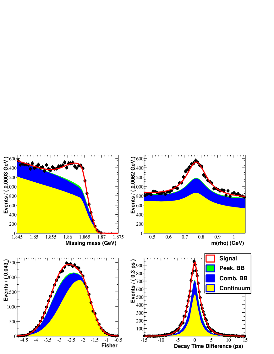
Figure 1: Projections of the PDF of partially reconstructed events onto the on-resonance data in the variables $m_{\rm miss}$ (upper left), $m(\rho)$ (upper right), $F$ (lower left), and $\Delta t$ (lower right). Events in the $\Delta t$ projection plot satisfy the additional criteria $m_{\rm miss}>1.854$ GeV, $0.6<m(\rho)<0.93$ GeV, and $F<-2.1$.

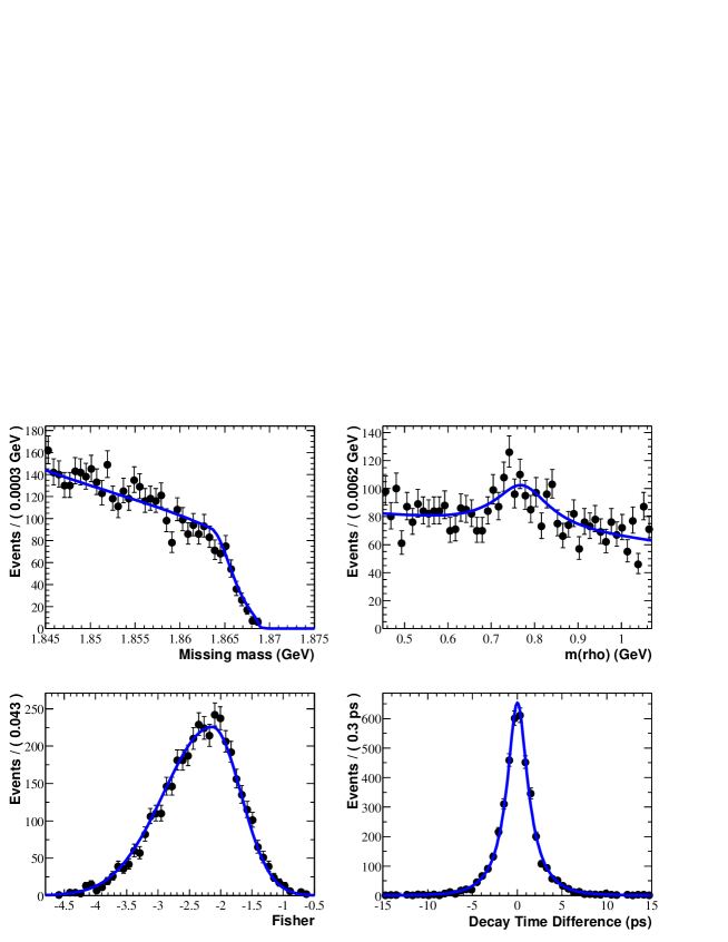
Figure 2: Projections of the PDF of continuum events onto the off-resonance data in the variables $m_{\rm miss}$ (upper left), $m(\rho)$ (upper right), $F$ (lower left), and $\Delta t$ (lower right).

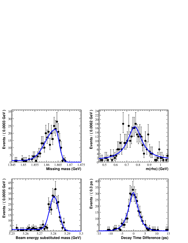
Figure 3: Projections of the PDF of fully reconstructed events onto the fully reconstructed data in the variables $m_{\rm miss}$ (upper left), $m(\rho)$ (upper right), $m_{\rm ES}$ (lower left), and $\Delta t$ (lower right).

Projections of the PDF onto the data are shown in Figs. 1 through 3. The result of the maximum likelihood $\Delta t$ fit is

$$\tau_{{}_{B^{0}}}^{\rm raw}=1.535\pm 0.064~{}{\rm(stat.)}~{}ps,$$ (9)

where the error is statistical only.

Several corrections are applied to this result, in order to account for known sources of bias. A correction of $+0.008\pm 0.011$ ps is due to the assignment of $a_{1}$ daughter tracks to the other $B$ vertex, decreasing the measured $\Delta t$ in ${\kern 1.79993pt\overline{\kern-1.79993ptB}{}^{0}\rightarrow{D^{*}}^{+}a_{1}^{-}}$ events. The resulting value of 1.543 ps is divided by $R_{D}=0.982\pm 0.022$, the ratio between the $B^{0}$ lifetime obtained from a fit to signal Monte Carlo events and the value obtained from a fit to the true $\Delta t_{t}$ distribution of this sample. This correction accounts for the effect of $D$ daughter tracks that pass the cone cut and are used in the other $B$ vertex. A correction of $+0.014\pm 0.013$ ps is applied to this result, to account for a possible bias due to event selection, determined by fitting the true $\Delta t_{t}$ distribution of signal events passing the selection criteria. The magnitudes and errors of all these corrections are obtained from the Monte Carlo simulation.

The fit PDF was used to generate and fit hundreds of Monte Carlo samples, each corresponding to the data sample in number of events and PDF parameters. The value of $\tau_{{}_{B^{0}}}$ obtained from these fits was on average lower than the generated value by $0.031\pm 0.005$ ps. Repeating these studies with different Monte Carlo sample sizes, this bias is understood to be due to limited sample statistics. A correction of this magnitude is therefore added to the value of $\tau_{{}_{B^{0}}}$. The fully corrected result is

$$\tau_{{}_{B^{0}}}=1.616\pm 0.064~{}{\rm(stat.)~{}ps}.$$ (10)

5 Systematic Errors and Cross Checks

Table 2: Systematic errors.

Source	Error (ps)
Statistical error of sideband fit	$0.033$
Statistical error of kinematic fit	$0.029$
Statistical error of wrong-sign fit	$0.002$
Monte Carlo statistics: Calculation of $R_{D}$	$0.036$
Monte Carlo statistics: Kinematic parameter fits	$0.014$
Monte Carlo statistics: Event selection bias	$0.013$
Monte Carlo statistics: ${\kern 1.79993pt\overline{\kern-1.79993ptB}{}^{0}\rightarrow{D^{*}}^{+}a_{1}^{-}}$ bias	$0.011$
$N^{D}_{\rm tr}$ uncertainty	$0.026$
Level of $\overline{B}\rightarrow D^{**}\rho^{-}$ background	$0.023$
Likelihood fit bias	0.016
Variation of fixed parameters	$0.015$
${\cal B}({\kern 1.79993pt\overline{\kern-1.79993ptB}{}^{0}\rightarrow{D^{*}}^{+}a_{1}^{-}})/{\cal B}(\kern 1.79993pt\overline{\kern-1.79993ptB}{}^{0}\rightarrow{D^{*}}^{+}\rho^{-})$	$0.005$
Level of peaking background	$0.003$
Bias from fully reconstructed events	$0.001$
SVT misalignment	$0.008$
$z$-length scale uncertainty	$0.007$
Beam energies uncertainty	$0.002$
Total	$0.075$

Several sources of systematic error are considered. The statistical error matrix obtained from the wrong-sign signal region $\Delta t$ fit is used to vary the parameters of the peaking $B^{0}{\kern-1.60004pt\kern 1.79993pt\overline{\kern-1.79993ptB}{}^{0}}$ background, taking into account their correlations. A fit to the right-sign signal region data follows each variation in these background parameters. The resulting variations in $\tau_{{}_{B^{0}}}$ are added in quadrature to form the total systematic error due to the finite number of events in the wrong-sign sample. With the same procedure, the errors due to the sideband fit are propagated to the wrong-sign signal region and then to the right-sign signal region fits, to obtain the error due to the sideband sample size. The errors due to the finite number of events used in the kinematic variable fits on data and the Monte Carlo simulation are evaluated in the same way.

The Monte Carlo statistical errors in the determination of $R_{D}$, the ${\kern 1.79993pt\overline{\kern-1.79993ptB}{}^{0}\rightarrow{D^{*}}^{+}a_{1}^{-}}$ bias, and the selection bias corrections are taken into account. The fraction of events in which $D$ daughter tracks are used in the other $B$ vertex fit is varied by $\pm 5\%$. The magnitude of this variation is determined by comparing the $N^{D}_{\rm tr}$ distributions of fully reconstructed data and Monte Carlo events. The resulting variation in $R_{D}$ is used to evaluate the systematic error due to this uncertainty.

The contribution of the $\overline{B}\rightarrow D^{**}\rho^{-}$ background is neglected in the fits. To evaluate the systematic error associated with this, we instead take the number of $\overline{B}\rightarrow D^{**}\rho^{-}$ in the data sample to be 2400, corresponding to ${\cal B}(\overline{B}\rightarrow D^{**}\rho^{-})\;{\cal B}({D^{**}}\rightarrow D^{*+}\pi)=0.3\%$. This value is estimated from known branching fractions of the decays $\overline{B}\rightarrow D^{**}\pi^{-}$, $\overline{B}\rightarrow D^{(*)}\rho^{-}$, $\overline{B}\rightarrow D^{(*)}\pi^{-}$, and available limits on ${\cal B}(\overline{B}\rightarrow{D^{**}}\rho^{-})$ [8]. The PDF parameters of this background are taken from the Monte Carlo simulation. Repeating the $\Delta t$ fit yields a 0.023 ps change in the value of $\tau_{{}_{B^{0}}}$, which is taken as the systematic error. The ${D^{**}}$ states simulated are $D_{1}(2420)$, $D_{2}^{*}(2460)$, and $D_{1}(j={1\over 2})$, the latter having mass 2.461 GeV and width 290 MeV. No significant difference is found between these states in terms of their effect on the observable quantities of this analysis.

Two variations of the signal $\Delta t$ PDF are used in fits to the data. In one variation, the parameter $b$ in Eq. (7) is replaced by $b\sigma_{{}_{\Delta t}}$. In the other, the sum of the narrow and wide Gaussians of Eq. (6) is replaced by a Gaussian convoluted with an exponential. The effect of generating Monte Carlo event samples using one PDF and fitting them using another PDF was studied. Based on these data and Monte Carlo studies, a systematic error of $0.016$ ps is estimated due to the choice of signal $\Delta t$ PDF.

The parameters $s$ and $b$ (Eq. (7)) of the signal and continuum PDF outlier Gaussians are fixed in the fit to the right-sign signal region data. To estimate the associated systematic errors, their values are varied within reasonable ranges, and the resulting changes in $\tau_{{}_{B^{0}}}$ are taken as systematic errors.

Additional systematic errors are due to the uncertainty in the relative branching fractions of ${\kern 1.79993pt\overline{\kern-1.79993ptB}{}^{0}\rightarrow{D^{*}}^{+}a_{1}^{-}}$ and $\kern 1.79993pt\overline{\kern-1.79993ptB}{}^{0}\rightarrow{D^{*}}^{+}\rho^{-}$, the level of peaking background, the introduction of a possible bias due to the use of fully reconstructed events, detector alignment and $z$-length calibration, and beam energy uncertainty. The total systematic error is 0.075 ps, dominated by the errors due to sideband and kinematic fit statistical errors, and Monte Carlo statistical errors. The systematic errors are listed in Tab. 2.

Several cross-checks were conducted to ensure the validity of the result. The number of signal events detected is in good agreement with the published branching fraction [8] and our signal reconstruction efficiency. The fit was repeated with different values of the cone cut, ranging between 0.6 and 1.2 radians. The data were fitted in bins of the lab frame polar angle, azimuthal angle, and momentum of the $\pi_{h}$, and in sub-samples corresponding to different SVT alignment calibrations. In all cases, no significant variation of the result was observed.

6 Conclusion

In a sample of 22.7 million $B\kern 1.79993pt\overline{\kern-1.79993ptB}{}$ pairs, we identified $5521\pm 252\pm 34$ $\kern 1.79993pt\overline{\kern-1.79993ptB}{}^{0}\rightarrow{D^{*}}^{+}\rho^{-}$ and $691\pm 36\pm 4$ ${\kern 1.79993pt\overline{\kern-1.79993ptB}{}^{0}\rightarrow{D^{*}}^{+}a_{1}^{-}}$ events using partial and full $B$ reconstruction. These events were used to measure the $B^{0}$ lifetime, with the preliminary result being

$$\tau_{{}_{B^{0}}}=1.616\pm 0.064~{}{\rm(stat.)}\pm 0.075~{}{\rm(syst.)~{}ps}.$$ (11)

This result is in good agreement with earlier published measurements [8], constituting a necessary step in validating the use of partially reconstructed $\kern 1.79993pt\overline{\kern-1.79993ptB}{}^{0}\rightarrow{D^{*}}^{+}\rho^{-}$ events for the measurement of $\sin(2\beta+\gamma)$.

Acknowledgements

We are grateful for the extraordinary contributions of our PEP-II colleagues in achieving the excellent luminosity and machine conditions that have made this work possible. The success of this project also relies critically on the expertise and dedication of the computing organizations that support BABAR. The collaborating institutions wish to thank SLAC for its support and the kind hospitality extended to them. This work is supported by the US Department of Energy and National Science Foundation, the Natural Sciences and Engineering Research Council (Canada), Institute of High Energy Physics (China), the Commissariat à l’Energie Atomique and Institut National de Physique Nucléaire et de Physique des Particules (France), the Bundesministerium für Bildung und Forschung (Germany), the Istituto Nazionale di Fisica Nucleare (Italy), the Research Council of Norway, the Ministry of Science and Technology of the Russian Federation, and the Particle Physics and Astronomy Research Council (United Kingdom). Individuals have received support from the A. P. Sloan Foundation, the Research Corporation, and the Alexander von Humboldt Foundation.

References

- [1] P.F. Harrison and H.R. Quinn (ed.), BABAR Physics Book, Chap. 7.6 (1998); R.G. Sachs, Enrico Fermi Institute Report, EFI-85-22 (1985) (unpublished); I. Dunietz and R.G. Sachs, Phys. Rev. D37, 3186 (1988) [E: Phys. Rev. D39, 3515 (1989)]; I. Dunietz, Phys. Lett. B427, 179 (1998).
- [2] N. Cabibbo, Phys. Rev. Lett. 10, 531 (1963); M. Kobayashi and T. Maskawa, Prog. Theoret. Phys. 49, 652 (1973).
- [3] The BABAR Collaboration, B. Aubert et al., Nucl. Instr. and Methods A479, 1 (2002).
- [4] The CLEO Collaboration, G. Brandenburg et al., Phys. Rev. Lett. 80, 2762 (1998).
- [5] The CLEO Collaboration, ICHEP98 852, CLEO CONF 98-23 (1998).
- [6] G. Fox and S. Wolfram, Phys. Rev. Lett. 41, 1581 (1978).
- [7] The ARGUS Collaboration, H. Albrecht et al., Phys. Lett. B254, 288 (1991).
- [8] See, for example, The Particle Data Group, C. Caso et al., Review of Particle Physics, Eur. Phys. J. C15, 606 (2000).