First electron beam polarization measurements with a Compton polarimeter at Jefferson Laboratory

Abstract

A Compton polarimeter has been installed in Hall A at Jefferson Laboratory. This letter reports on the first electron beam polarization measurements performed during the HAPPEX experiment at an electron energy of 3.3 GeV and an average current of 40 $\mu$A.

The heart of this device is a Fabry-Perot cavity which increased the luminosity for Compton scattering in the interaction region so much that a $1.4\%$ statistical accuracy could be obtained within one hour, with a $3.3\%$ total error.

I Introduction

Nuclear physics experiments using a polarized electron beam require an accurate knowledge of the beam polarization. However, polarization measurements often account for the main systematic uncertainty for such experiments. The Continuous Electron Beam Accelerator Facility (CEBAF), located at Jefferson Laboratory (JLab), is equipped with three types of beam polarimeters. A Mott polarimeter, limited to low energy (few MeV), is available at the injector, while Møller polarimetry is used at low currents (few $\mu$A) in all three experimental halls. The main limitation of both techniques is their invasive character due to the solid target (Au and Fe, respectively) used, preventing beam polarization measurements simultaneous to running an experiment. Moreover, neither of these instruments is capable of operating in the energy and/or current regime delivered at JLab. In contrast, Compton polarimetry, which uses elastic scattering of electrons off photons, is a non-invasive technique. Indeed, the interaction of the electron beam with the ”photon target” does not affect the properties of the beam so that the beam polarization can be measured upstream of the experimental target simultaneously with running the experiment. The applicability of Compton polarimetry has been demonstrated at high-current ($>$ 20 mA) storage rings (NIKHEF [2], HERA [3]) and at high-energy ($>$ 50 GeV) colliders (SLAC [4], LEP [5]). However, at the CEBAF beam conditions (energy of several GeV, current of up to 100 $\mu$A) the Compton cross section asymmetry is reduced to a few percent, which makes Compton polarimetry extremely challenging.

A pioneering technique was selected to increase the Compton interaction rate such that a 1% statistical error measurement could be achieved within an hour: an optical Fabry-Perot type cavity fed by an infrared photon source. The Compton luminosity has been enhanced further by minimizing the crossing angle between the electron and the photon beams, which required setting the cavity mirrors only 5 mm away from the electron beam. This unique configuration allows measurements of the electron beam polarization at moderate beam energies ($>$ 1 GeV) and currents ($>$ 10 $\mu$A). The Fabry-Perot cavity [6], comprising two identical high- reflectivity mirrors, amplifies the photon density at the Compton Interaction Point (CIP) with a nominal gain of 7000. The initial laser beam (NdYAG, 300 mW, 1064 nm) is locked on the resonant frequency of the cavity through an electronic feedback loop [7]. The optical cavity, enclosed in the beam pipe, is located at the center of a magnetic chicane (16 m long), consisting of 4 identical dipoles. The chicane separates the scattered electrons and photons and redirects the primary electron beam unchanged in polarization and direction to the Hall A beam line. The backscattered photons are detected in a matrix of 25 PbWO₄ crystals [8], which are read out by PMT’s. The PMT output signal is amplified and integrated before being sent to ADC’s. This article reports on the first polarization measurements performed during the second part of the data taking of HAPPEX experiment [9] (July 1999) with the Hall A Compton polarimeter at an electron energy of 3.3 GeV and an average current of 40 $\mu$A.

II Towards a polarization measurement

For the HAPPEX experiment CEBAF produced a longitudinally polarized electron beam with its helicity flipped at 30 Hz. This reversal induces an asymmetry, $A_{exp}=\frac{N^{+}-N^{-}}{N^{+}+N^{-}}$, in the Compton scattering events $N^{\pm}$ detected at opposite helicity. In the following, the events are defined as count rates normalized to the electron beam intensity within the polarization window. The electron beam polarization is extracted from this asymmetry via [10]

$$P_{{e}}=\frac{A_{exp}}{P_{\gamma}A_{{th}}},$$ (1)

where $P_{\gamma}$ denotes the polarization of the photon beam and $A_{{th}}$ the analyzing power. The measured raw asymmetry $A_{raw}$ has to be corrected for dilution due to the background-over-signal ratio $\frac{B}{S}$, for the background asymmetry $A_{B}$ and for any helicity-correlated luminosity asymmetries $A_{F}$, so that $A_{exp}$ can be written to first order as

$$A_{exp}=\left(1+\frac{B}{S}\right)A_{raw}-\frac{B}{S}A_{B}+A_{F}.$$ (2)

The polarization of the photon beam can be reversed with a rotatable quarter-wave plate, allowing asymmetry measurements for both photon states, $A_{raw}^{(R,L)}$. The average asymmetry is calculated as

$$A_{exp}=\frac{\omega_{R}A_{raw}^{R}-\omega_{L}A_{raw}^{L}}{\omega_{R}+\omega_{L}},$$ (3)

where $\omega_{R,L}$ denote the statistical weights of the raw asymmetry for each photon beam polarization. Assuming that the beam parameters remain constant over the polarization reversal and that $\omega_{R}\simeq\omega_{L}$, false asymmetries cancel out such that

$$\displaystyle A_{exp} \simeq \frac{A_{raw}^{R}-A_{raw}^{L}}{2}(1+\frac{B}{S}).$$ (4)

III Data taking and event preselection

Before starting data taking, the electron beam orbit and its focus in the central part of the chicane have to be optimized to reduce the background rate observed in the photon detector which was generated by a halo of the electron beam scraping on the Fabry-Perot mirror ports [12]. The vertical position of the electron beam was adjusted until the overlap between the electron and the photon beam was maximized at the CIP. This was achieved by measuring the count rate in the photon detector while adjusting the field of the chicane dipoles. Because of a slow drift of the electron beam, its position had to be readjusted every couple of hours to minimize systematic effects (cf section IV). Polarimetry data were accumulated continuously while running the HAPPEX experiment. Each one hour run consisted of five pairs of signal - with the cavity resonant (cavity ON) - and background - when the cavity was intentionally unlocked (cavity OFF), approximatively one third of the time - runs. Signal and background events were recorded for alternating values of the photon beam polarization inside the cavity. With an average power of 1200 W inside the cavity, the count rate observed in the photon detector was $\sim$ 90 kHz and the background rate of the order of 16 kHz.

For the data presented here, only the central crystal was used in the backscattered photon detection. The electronics was triggered when the amplitude of a signal recorded in the PMT coupled to that central crystal exceeded a preset threshold value. The state (Cavity ON/Cavity OFF) of a recorded event is determined by the photon beam diagnostics outside the cavity and by the cavity-locking feedback parameters [7]. The first event selection imposed a minimum current of 5 $\mu$A and variations smaller than 3 $\mu$A within each run as well as minor cuts to account for malfunctions of the experimental setup. The modulation of the electron beam position and energy [9] imposed by the HAPPEX experiment induced a significant loss of events ($\sim$ 36 %) in limiting systematic effects (cf section IV).

IV Experimental asymmetry

The raw asymmetry normalized to the electron beam intensity, $A_{raw}$, is determined at 30 Hz for each pair of opposite electron helicity states. Averaging all pairs for both photon polarizations yields the mean raw asymmetry (eq. 3) The mean rates with cavity ON ($r^{1}$) and cavity OFF ($r^{0}$) are obtained by averaging over both electron and both photon states within each run. The dilution factor of the asymmetry is thus $(1+\frac{B}{S})=\frac{r^{1}}{r^{1}-r^{0}}$. The average signal and background rates were respectively about 1.9 and 0.4 kHz/$\mu$A. The experimental asymmetry of about $0.013$ was determined with a relative statistical accuracy $\sim$ 1.4% within an hour. Fluctuations of the signal over background ratio $\frac{B}{S}$ and of the statistical precison of the background asymmetry estimation $A_{B}$ within a run account for a small contribution to the error budget (cf table I).

Any correlation between the Compton scattering luminosity and the electron helicity induces a false asymmetry which adds to the physical asymmetry (eq. 2). For each pair $i$ of opposite electron helicity, a systematic difference of the transverse electron beam position or angle $\Delta p_{i}=\frac{p_{i}^{+}-p_{i}^{-}}{2}$ ($p_{i}=x,y,\theta_{x},\theta_{y}$) gives rise to an asymmetry

$$A_{p}^{i}=\left.\frac{1}{r^{i}(p=p_{i})}\frac{\partial r^{i}}{\partial p}\right|_{i}\Delta p_{i},\quad\text{with}\quad r^{i}=\frac{N_{i}}{t_{i}I_{i}}.$$ (5)

The two beams, crossing in the horizontal plane, each have a transverse size of $\sim$ 100 $\mu$m. The Compton luminosity is therefore highly sensitive to the vertical position of the electron beam (fig. 1), of the order of 0.2%/$\mu$m. Thus, a systematic position difference of $\sim$ 100 nm would generate a false asymmetry of 0.02%, corresponding to $\sim$ 1.5% of the experimental asymmetry. To minmize the systematic error, the second event selection accepts only data lying within 50 $\mu$m from the luminosity optimum. Again, averaging over the two helicity states of the photon beam cancels this contribution if the beam properties remain stable over the duration of the run. However, a slow drift of the beam parameters induces a change in the count rate sensitivity. The asymmetry induced by a difference $\Delta p_{i}$ can therefore be different for the two photon states, thus creating a residual false asymmetry. This residual contribution is estimated by calculating $A_{p}^{i}$ for each pair and summing over the four positions and angles. Averaging over all pairs is done using the statistical weights of the experimental asymmetry. Helicity-correlated false asymmetries represent on average 1.2% of the experimental asymmetry and remain its main source of systematic error (cf table I).

V Photon beam polarization

The photon beam polarization can not be measured at the CIP during the experiment since any instrument placed in the photon beam interrupts the build-up process. Instead, the polarization at the exit of the cavity was monitored on-line during data taking. Absolute polarization measurements were performed at the CIP and at the exit of cavity during maintenance periods when the cavity is removed. These measurements allow to model the transfer function of the light from the CIP to the outside detectors, which then result in an evaluation of the photon beam polarization during the experiment [11]. The polarization is found to be $P_{\gamma}^{R,L}=\pm 99.3^{+0.7}_{-1.1}\%$, for both right- and left-handed photons.

VI Analyzing Power

The Compton scattering cross section has to be convoluted with the response function of the calorimeter:

$\displaystyle\frac{d\sigma^{\pm}_{smeared}}{dk_{r}^{\prime}}=\int^{\infty}_{o}\frac{d\sigma^{\pm}_{c}}{dk^{\prime}}\,g(k^{\prime}-k^{\prime}_{r})\,dk^{\prime}$

where $k^{\prime}$ is the backscattered photon energy, $k^{\prime}_{r}$ is the energy deposited in the calorimeter, $\frac{d\sigma^{\pm}_{c}}{dk^{\prime}}$ is the helicity-dependent Compton cross section and $g(k^{\prime})$ is the response function of the calorimeter. The latter is assumed to be gaussian with a width $\sigma_{res}(k^{\prime})=a\oplus b/\sqrt{k^{\prime}}\oplus c/k^{\prime}$ where $(a,b,c)$ are fitted to the data. The observed energy spectrum (fig. 2) has a finite width at the threshold. This can be due either to the fact that the threshold level itself oscillates or to the fact that a given charge can correspond to different voltage amplitudes at the discriminator level. To take this into account the threshold is modelled using an error function $p(k^{\prime}_{s},k^{\prime}_{r})=erf(\frac{k^{\prime}_{r}-k^{\prime}_{s}}{\sigma_{s}})$ in which $\sigma_{s}$ is fitted to the data. Hence, the observed count rate can be expressed as :

$\displaystyle N^{\pm}(k^{\prime}_{s})={\cal{L}}\times\int^{\infty}_{0}p(k^{\prime}_{s},k^{\prime}_{r})\,\frac{d\sigma^{\pm}_{smeared}}{dk_{r}^{\prime}}\,dk^{\prime}_{r}$

where $\cal{L}$ is the interaction luminosity. An example of a measured energy spectrum and a fit using the procedure described in this section is shown in fig. 2. Finally, the analyzing power of the polarimeter can be calculated:

$\displaystyle A_{th}=\frac{N^{+}(k^{\prime}_{s})-N^{-}(k^{\prime}_{s})}{N^{+}(k^{\prime}_{s})+N^{-}(k^{\prime}_{s})}$

and is of the order of 1.7 %. In calculating the energy spectrum, the raw ADC spectrum had to be corrected for non-linearities in the electronics, resulting in a systematic error of 1 %. Another 1 % comes from the uncertainty in the calibration which is performed by fitting the Compton edge. Variations of the parameter $a,\,b,\,c,\,k^{\prime}_{s},\,\sigma_{s}$ around the fitted values where used to estimate the systematic error associated with our imperfect modelling of the calorimeter response. This contributes 1.9% to the systematic error which is mainly due to the high sensitivity of the analyzing power to the value of the threshold ($\sim$ 1%/MeV around 30 MeV). This represents the main source of systematics in our measurement (cf table I).

VII Results and conclusions

We have measured for the first time the JLab electron beam polarization at an electron energy of 3.3 GeV and an average current of 40 $\mu$A. The 40 measurements of the electron beam polarization, which was of the order of 70% [12], are displayed in fig. 3. The average error budget for these data is given in table I. These results are in good agreement with the measurements performed with the Hall A Møller polarimeter [13]. Moreover, the Compton polarimeter provides a relative monitoring of the polarization with an error of 2% due to the absence of correlations between consecutive runs in the systematic errors associated with the photon detector ($A_{th}$) and with the photon polarization ($P_{\gamma}$). These results show that the instrument presented here is indeed capable of producing a fast and accurate polarization measurement. The challenging conditions of JLab (100 $\mu$A, few GeV) have been succesfully adressed with a low-power laser coupled to a Fabry-Perot cavity. Moreover, the level of systematic uncertainties reached in these first measurements, is encouraging for forth-coming achievements. Several hardware improvements have been added to the setup since then: new front-end electronic cards, feed-back on the electron beam position and a detector for the scattered electron, consisting of 4 planes of 48 micro-strips. Data taken during recent experiments [14] [15] are being analyzed and are expected to reach a 2% total error at 4.5 GeV and 100 $\mu A$.

VIII Acknowledgments

The authors would like to acknowledge Ed Folts and Jack Segal for their constant help and support, as well as the Hall A staff, the HAPPEX and Hall A collaboration and the Accelerator Operations group. This work was supported by the French Commissariat à l’Energie Atomique (CEA) and the Centre National de la Recherche Scientifique (CNRS/IN2P3). The Southern Universities Research Association (SURA) operates the Thomas Jefferson National Accelerator Facility for the US Department of Energy under Contract No. DE-AC05-84ER40150.

TABLE I.: Average relative error budget.

Source			Systematic	Statistical
$P_{\gamma}$			1.1%
$A_{exp}$	Statistical			1.4%
	$B/S$	0.5%
	$A_{B}$	0.5%	1.4%
	$A_{{F}}$	1.2%
$A_{{th}}$	Non-linearities	1%
	Calibration	1%	2.4%
	Efficiency/Resolution	1.9%
Total			3.0%	1.4%

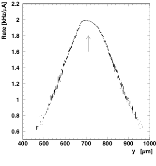
FIG. 1.: Count rate normalized to the beam current versus vertical position of the electron beam.

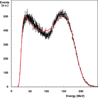
FIG. 2.: Energy spectrum of Compton photons, detected in the central PbWO₄ crystal. The solid curve is the fit, which accounts for the calorimeter resolution and efficiency.

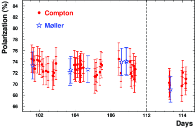
FIG. 3.: Polarization measured by the Compton (full circles) and the Møller (stars) polarimeters during the HAPPEX experiment. For the Møller data the total error is shown, for the Compton the statistical and total error is indicated separately.

REFERENCES

- [1] Corresponding author.
- [2] I. Passchier et al., Nucl. Instr. Meth. A 414, 446 (1998).
- [3] D.P. Barber et al., Nucl. Instr. Meth. A 329, 79 (1993).
- [4] M. Woods, Proc. of the Workshop on High Energy Polarimeters, Amsterdam, 1996, eds. C.W. de Jager et al., p. 843.
- [5] D. Gustavson et al., Nucl. Instr. Meth. A 165, 177 (1979).
- [6] J.P. Jorda et al., Nucl. Instr. Meth. A 412, 1 (1998).
- [7] N. Falletto et al., Nucl. Instr. Meth. A 459, 412 (2001).
- [8] D. Neyret, T. Pussieux et al., Nucl. Instr. Meth. A 443, 231 (2000).
- [9] K. A. Aniol et al. [HAPPEX Collaboration], Phys. Lett. B 509, 211 (2001).
- [10] C. Prescott, SLAC internal report, SLAC TN 73 1.
- [11] N. Falletto, Ph.D. thesis (in french), Université Grenoble I; Report CEA/DSM/DAPNIA/SPhN-99-03-T.
- [12] M. Baylac, Ph.D. thesis (in french), Université Lyon I ; Report CEA/DSM/DAPNIA/SPhN-00-05-T.
- [13] .
- [14] S. Frullani, J. Kelly and A. Sarty (spokespersons), JLab experiment E91-011.
- [15] E. Brash, M. Jones, C. Perdrisat and V. Punjabi (spokespersons), JLab experiment E99-007.