The multilevel trigger system of the DIRAC experiment

Abstract

The multilevel trigger system of the DIRAC experiment at CERN is presented. It includes a fast first level trigger as well as various trigger processors to select events with a pair of pions having a low relative momentum typical of the physical process under study. One of these processors employs the drift chamber data, another one is based on a neural network algorithm and the others use various hit-map detector correlations. Two versions of the trigger system used at different stages of the experiment are described. The complete system reduces the event rate by a factor of 1000, with efficiency $\geq$95% of detecting the events in the relative momentum range of interest.

, , , , , , , , , , , , , , , ,

1 Introduction

The DIRAC experiment [1] at CERN measures the lifetime of atoms consisting of $\pi^{+}$ and $\pi^{-}$ mesons ($A_{2\pi}$). This $A_{2\pi}$ lifetime is directly related to the difference $a_{0}-a_{2}$ between the $s$-wave $\pi\pi$ scattering lengths with isotope spin values 0 and 2.

This difference is calculated in the framework of the chiral perturbation theory with high precision but has not been measured experimentally with a corresponding accuracy yet. Theoretical calculations predict the $A_{2\pi}$ lifetime to be close to $3\cdot 10^{-15}$ s.

The experiment is using the 24 GeV proton beam from the PS accelerator at CERN. The DIRAC experimental setup (Fig. 1) is a magnetic spectrometer with detectors arranged in one upstream and two downstream arms. The spectrometer is placed in the secondary beam produced by the primary protons hitting a fixed target. The upstream part, along the secondary beam path before the dipole magnet, contains microstrip gas chambers (MSGC), a scintillating fiber detector (SFD) and a scintillation hodoscope (IH – ionization hodoscope). The downstream arms include drift chambers (DC), scintillation hodoscopes with vertically and horizontally oriented scintillators (VH and HH respectively), gas Cherenkov counters (Ch), preshower detectors (PSh) and finally muon counters (Mu) placed behind iron absorbers.

Figure 1: Schematic top view of the DIRAC spectrometer. MSGC – microstrip gas chambers, SFD – scintillating fibre detectors, IH – ionization hodoscopes, DC – drift chambers, VH,HH – vertical and horizontal hodoscopes, Ch – Cherenkov counters, PSh – preshower detectors, Mu – muon detectors.

The $A_{2\pi}$ disintegrate into pairs of oppositely charged pions with a very low relative momentum ($Q$), typically less than 3 MeV/$c$. Such pion pairs have to be efficiently detected for the measurement of the $A_{2\pi}$ lifetime.

Targets of different materials and thicknesses are used during data taking. For each target the beam intensity is adjusted to obtain an approximately constant counting rate. The PS delivers the beam in spills of duration 400–500 ms. With a typical proton beam intensity of $10^{10}$ p/spill and a $94\mu$ thick Ni target, single rates in the upstream detectors are about $3\cdot 10^{6}$ counts/spill whereas in the downstream detectors they are up to $8\cdot 10^{5}$ and $6\cdot 10^{5}$ counts/spill in the positive and negative arms respectively.

The trigger logic should provide a reduction of the event rate to a level acceptable to the data acquisition system. Pion pairs are produced in the target mainly in a free state with a wide distribution over their relative momentum $Q$. The on-line event selection rejects events with pion pairs having $Q_{L}>30\,$MeV/$c$ or $Q_{x}>3\,$MeV/$c$ keeping at the same time high efficiency for detection of pairs with $Q$ components below these values.

2 The trigger system

A multilevel trigger is used in DIRAC. It comprises a simple and fast first level trigger and several higher level trigger processors with different selection criteria for various components of the relative momentum of pion pairs.

Due to the requirements of the data analysis procedure the on-line selection of only real pion pairs originating from a single proton–target interaction is not enough. In addition, a large number of uncorellated, accidental, pion pairs are also necessary. These accidental pairs are used to reconstruct the relative momentum distribution for free (non-atomic) pion pairs without Coulomb interaction in the final state. The measurement of this distribution is indispensable for the correct calculation of the numbers of produced and detected $A_{2\pi}$. Therefore, within a preselected coincidence time window, the trigger system should apply very similar selection criteria for real and accidental coincidences. The statistical error of the $A_{2\pi}$ lifetime measurement depends on the numbers of both real and accidental detected pairs. The optimal ratio of real to accidental events at the present experimental conditions is achieved with a $\pm 20$ ns coincidence time window between the times measured in the left (VH1) and right (VH2) vertical hodoscopes.

The trigger scheme was upgraded since the start of the experiment. In this paper we present two trigger options: one was successfully used during the first year of data taking and another one is being currently used.

The block diagram of the trigger structure is presented in Fig. 2. In the diagram of Fig. 2a the first level trigger T1 in coincidence with the trigger T2 starts digitization of the detector signals in the data acquisition (DAQ) modules (ADC, TDC etc.). At the next level the OR of the trigger processors T3 and the neural network trigger DNA (DIRAC Neural Atomic trigger) selects further events by forcing additional constraints to the relative momentum. The triggers T2 and DNA start with a fast pretrigger (T0). A negative decision of T3 and DNA provokes clearing of all data buffers and the trigger and data acquisition systems return to the READY state. A positive decision of the T3+DNA logic starts the readout process.

Figure 2: General block diagram of the DIRAC multilevel trigger. Variants a and b were used at the earlier and later stages of the experiment, respectively.

In the latest option of the trigger system (Fig. 2b) a powerful drift chamber trigger processor T4 was added and the neural trigger DNA was upgraded to a DNA/RNA version (Revised Neural Atomic trigger) with improved performance. This made it possible to obtain better trigger selectivity and higher efficiency. Hence the T2 and T3 stages were not needed any more.

In addition to the mainstream trigger selection aimed at detecting pionic atoms, there are also several special calibration triggers which can be running in parallel with the main one or used separately for dedicated measurements. They start the DAQ directly, bypassing the selection of higher level triggers. When these triggers are used in parallel with the main one appropriate prescaling factors are implemented to maintain a reasonable total event rate. Any trigger stage higher than T1 can be disabled (set to a transparent mode).

3 Trigger 1

The first level trigger (T1) [2] fulfils the following tasks:

1. Selects events with signals in both detector arms downstream the magnet;

2. Classifies the particle in each arm as a pion or an electron. Protons and kaons are equally included in the “pion” class. Muons could be identified with the use of the muon detector. However this detector is only used for off-line analysis and special dedicated measurements;

3. Arranges the coincidences between the two arms. The coincidence time window defines the ratio between the real and accidental events in the collected data;

4. Applies a coplanarity cut for pion pairs: a difference between the hit slab numbers in the horizontal hodoscopes in the two arms (HH1 and HH2, respectively) should be $\leq 2$. This criterion determines selection for the $y$ component of the pair relative momentum;

5. Selects in parallel events from several physical processes needed for the setup calibration: e⁺e^- pairs, decays $\Lambda\rightarrow p+\pi^{-}$, $K^{\pm}$-decays to three charged pions, $\pi^{+}\pi^{-}$ pairs without the coplanarity cut.

All T1 modules are ECL line programmable multichannel CAMAC units. Most of them are commercial modules except the dedicated coplanarity processor developed at JINR. To reduce the time jitter of the trigger, meantimer units removing the dependence of timing on hit coordinate are used in all VH and HH channels.

The pion ($\pi 1,\pi 2$) and electron (e1,e2) signatures in each of the downstream arms are defined as a coincidence between different detectors:

$$\mathrm{VH1(2)}\cdot\mathrm{HH1(2)}\cdot\overline{\mathrm{Ch1(2)}}\cdot\mathrm{PSh1(2)}=\pi 1(\pi 2)$$

$$\mathrm{VH1(2)}\cdot\mathrm{HH1(2)}\cdot\mathrm{Ch1(2)}\cdot\mathrm{PSh1(2)}=\mathrm{e1(e2)}.$$

Here VH1, VH2 etc. denote the logical OR of all signals from the corresponding detector. The signatures from both arms are combined to produce the final first level trigger. The timing of “$\pi$” and “e” signals is defined by the vertical hodoscope of the corresponding arm, as the VH has the best time resolution among all detectors. At the trigger level VH slabs are aligned in time with an accuracy of 1 ns. Further off-line time corrections provide 175 ps resolution for the time difference between the signals in the two arms.

The definitions of the subtriggers are the following.

• The pion pair “atomic” trigger: $A_{2\pi}=\pi 1\cdot\pi 2\cdot\mathrm{Copl}$ , where “Copl” is the positive decision of the coplanarity selection processor. The coplanarity processor (15 ns decision time) reduces the trigger rate by a factor of 2.

• The electron pair trigger: ${\mathrm{e}^{+}\mathrm{e}^{-}=\mathrm{e}1\cdot\mathrm{e}2}$.

• The pion pair trigger (no coplanarity selection): $\pi^{+}\pi^{-}=\pi 1\cdot\pi 2$.

• The $\Lambda$-decay trigger $\Lambda\rightarrow p+\pi^{-}$:

  $$\Lambda=(\mathrm{VH}1[17]\cdot\mathrm{HH}1\cdot\overline{\mathrm{Ch1}}\cdot\mathrm{PSh1})(\mathrm{VH}2[1\div 16]\cdot\mathrm{HH}2\cdot\overline{\mathrm{Ch2}}\cdot\mathrm{PSh2}).$$

  As a matter of fact, this is the same definition as that for the $\pi^{+}\pi^{-}$ trigger but here only vertical hodoscope slab 17 in VH1 and slabs $1\div 16$ in VH2 out of the total 18 slabs of each arm are used. This reflects the kinematics of $\Lambda$-decay where the proton (in arm 1) and the $\pi^{-}$ (in arm 2) hit very different VH slab ranges.

• The $K$-decay trigger ($K^{+}\rightarrow\pi^{+}\pi^{+}\pi^{-}$, $K^{-}\rightarrow\pi^{-}\pi^{-}\pi^{+}$):

  $$\mathrm{K}=\pi 1\cdot\pi 2\cdot Maj[\mathrm{VH}\geq 3]\cdot Maj[\mathrm{HH}\geq 3]\cdot Maj[\mathrm{VH}<5],$$

  where $Maj$ denotes the majority logic applied to the number of hits in the slabs of both VH or both HH hodoscopes. Thus, from the pions detected in two arms only the events with at least 3 particles in the downstream detectors are selected and at the same time too complicated events with a high multiplicity $\geq 5$ are rejected. Simultaneous majority selection in the vertical VH and horizontal HH hodoscopes helps to suppress edge-crossing of the adjacent hodoscope slabs by single particles which could imitate the passage of two independent particles in one hodoscope.

For the last two subtriggers ($\Lambda$ and $K$) the coincidence time window is reduced by a factor of 2.5 as there is no need to collect accidental events for these categories. It is evident that the $\Lambda$- and $K$-triggers do not provide detection of clean $\Lambda$ and $K$ events but they enhance their proportions in the final data sample.

The block diagram of the combination of various subtriggers is shown in Fig. 3. All signals pass through the mask register and after prescaling are combined with an OR function. Any subtrigger can be enabled or disabled by proper programming of the mask register. Timing of all subtriggers is the same. Independent prescaling of each subtrigger channel allows one to adjust the relative rates and to keep the ratio of the main and calibration trigger rates at an optimum level. A specific trigger mark is recorded for every event, so the data can be sorted by trigger type at the off-line analysis and on-line monitoring.

Figure 3: Combination of different subtrigger modes in the 1st level trigger.

The final first level trigger signal T1, as shown in Figs. 2a and 2b, initiates operation of the DAQ modules (gating of ADC, starting of TDC etc.) either directly or after a coincidence with the T2 decision. It also triggers higher level processors. Depending on the decisions of the trigger processors the event data will either be converted and moved to the data collection memories or discarded. During this period generation of a new T1 signal is inhibited.

4 Pretrigger T0

Some trigger processors, especially T2 and DNA/RNA, need a fast initial signal to start evaluating an event. An early fast pretrigger (T0) is provided for that purpose. It is a simple coincidence of signals from at least one slab in each of the VH1, VH2, PSh1 and PSh2 detectors, the coincidence time window being the same as for the T1 trigger ($\pm 20\,$ns). To obtain a T0 signal as early as possible the VH signals are taken directly from the discriminator outputs of the upper PMs, i.e. before the meantimers. As a consequence, T0 has a 3 ns jitter which disappears in the final trigger due to further coincidence of various decisions with T1.

5 Trigger 2

Trigger 2 (its general ideas are considered, in particular, in [3]) uses the upstream SFD and IH detectors to select pairs with small distances along the $x$ direction ($\Delta x$). This leads to rejection of events with a high component of the relative momentum along $x$ ($Q_{x}$). Typical relative momenta of pions from the $A_{2\pi}$ breakup correspond to particle distances $\Delta x\leq 9$ mm in the upstream detectors.

The T2 trigger includes three independent modes combined by an OR function (Fig. 4): in Mode 1  and Mode 2  the data from two IH planes (A and B) are used and in Mode 3  the information from SFD is evaluated. Only the X-planes of each detector are used.

Figure 4: Different T2 trigger modes. Mode 1: $\Delta x\leq 6$ mm in one plane. In two staggered planes $\Delta x\leq 3$ mm. Mode 2: $\Delta x\leq 12$ mm. Mode 3: $\Delta x\leq 9$ mm.

Mode 1 selects events with two charged particles hitting the same slab in the plane X-A of IH and the corresponding element in the plane X-B. Selection of double hits is based on charge discrimination with a threshold corresponding to detection of double ionization. An IH scintillator slab is 6 mm wide, therefore a double ionization signal in a plane arises if $\Delta x\leq 6$ mm. However the plane X-B is shifted with respect to X-A by half-width of a slab, hence only particle pairs with $\Delta x\leq 3$ mm are accepted by Mode 1.

To ensure the same selection efficiency for two uncorrelated particles as for pions originating from a $A_{2\pi}$ breakup, dedicated integrators have been designed and implemented in all IH channels of the X-planes. The integration is started by T0. The integrator accumulates the input charge during a preset time interval and then compares it with the double ionization threshold.

The outputs of the double ionization threshold discriminators are connected to a trigger logic circuit (TLC) which requires a coincidence between the double ionization signal from a slab in the plane X-A with a signal from the matching slab in X-B. As the slabs in the planes X-A and X-B are staggered, the coincidence in TLC is performed for two possible matching combinations.

In Mode 2 hits (of any amplitude over the single ionization level) in adjacent slabs of planes A or B of IH are required. This mode accepts the events with $\Delta x\leq 12$ mm.

Mode 3 provides independent selection of events with small $\Delta x$ using the SFD [4]. Signals from the fiber columns (the fiber diameter is 0.5 mm) of the SFD X-plane after peak-sensitive discriminators [5] are coupled in pairs and come to a SFD trigger logic circuit (TLC). TLC tests if hits with distance $x\leq$9 mm are present in the SFD hit pattern. This value of the $\Delta x$ interval has been chosen as it coincides exactly with the range of distances for pions from $A_{2\pi}$ dissociation (the distance range in TLC can be varied from 1 to 15 mm). However, the SFD trigger efficiency drops at $\Delta x<1$ mm as the tracks cannot be resolved when two particles hit the same fiber column or a pair of adjacent coupled columns.

Decisions of all 3 modes are combined with an OR function in order to increase the trigger efficiency: Mode 1 recuperates the events rejected by Mode 3 due to very small $\Delta x$, Mode 1 and Mode 2 compensate inefficiency of the SFD detector itself (which is not negligible) while Mode 3 recovers the events lost by Mode 1 and Mode 2 due to presence of small gaps between the IH scintillators.

The resulting global T2 signal is synchronized with a delayed T0 signal; this decreases the time jitter of T2 decisions down to the 3 ns jitter of T0. In further coincidence with T1 the timing of T1$\cdot$T2 is defined by the T1 signal.

The selection efficiency for low $Q$ events of T2 is around 90–95%, and its rejection power is about 1.3–1.4. Both numbers vary slightly according to the beam conditions (beam time structure and background level).

6 Trigger 3

Further rejection of high $Q$ events is provided by the T3 processor. Its implementation initially considered in [6] is presented in detail in [7]. T3 makes a fast analysis of hit patterns in the vertical hodoscopes VH1, VH2 and the ionization hodoscope IH.

For pairs with low longitudinal component of the relative momentum ($Q_{L}$) there is a correlation between the hits in VH1 and VH2 (see Fig. 5): for any slab hit in VH1 there is a limited group of slabs in VH2 where the corresponding hit could be found. The algorithm becomes much more selective if the information about the slabs hit in the ionization hodoscope IH is additionally used to define the particle’s X-coordinates before the magnet (obtained from IH hit slab numbers) and consequently indicate the appropriate VH1–VH2 correlation map. T3 applies a $Q_{L}\leq 30\,$MeV/$c$ cut in its current configuration.

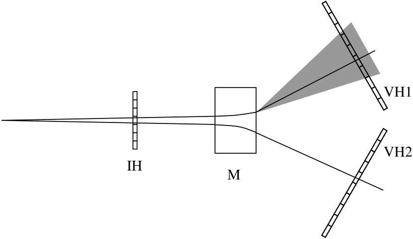
Figure 5: Logic of the T3 selection.

The input data for T3 are two 18-bit patterns from the meantimers of the VH1 and VH2 hodoscopes and a 16-bit pattern from IH. The IH pattern used is produced by the logic of the double ionization event selection (as in T2). It provides the X-coordinate region(s) where double ionization in one slab or two hits in adjacent slabs are detected (similar to Mode 1+Mode 2 of T2 but requesting double ionization in any of the IH X-planes).

The T3 logic is based on LeCroy Universal Logic Module 2366. The Xilinx FPGA (Field Programmable Gate Array technology) chip of this module has been programmed with the corresponding trigger algorithm. The implemented correlation maps of the VH1, VH2 and IH signals were obtained with Monte-Carlo simulation of the DIRAC setup and further tested with real experimental data.

The module configuration is stored in a binary file. Before data taking it is loaded into the Xilinx chip via the CAMAC bus. Files with different configurations may be downloaded to adapt the T3 performance to specific needs. The input signals to T3 are latched by T1 (or T1$\cdot$T2) and 120 ns later the decision of T3 about the event is delivered.

There is also a special “transparent” T3 operation mode. A signal in the dedicated “transparent” input forces T3 to accept the event. This mode is used for calibration triggers ($e^{+}e^{-}$, $\Lambda$ etc.) when there should be no event suppression by T3: these event flags come into the “transparent” input and hence prevent the event from being probably rejected.

The T3 rejection power for typical experimental conditions is around 2.0 with respect to T1. The T3 efficiency for pairs with $Q_{x}\leq 3\,$MeV/$c$, $Q_{y}\leq 3$ MeV/$c$ and $Q_{L}\leq 30\,$MeV/$c$ is 97%.

7 DNA and RNA neural network triggers

The DNA (DIRAC Neural Atomic) trigger [8] is a processing system based on a neural network algorithm. The DNA hardware is based on the custom-built version of the neural trigger used initially in the CPLEAR experiment [9]. The flexibility of the implemented algorithm allowed the system to be incorporated in the DIRAC trigger system too.

DNA receives the hit patterns from the vertical hodoscopes VH1, VH2, the X-planes of the ionization hodoscope IH and optionally the preshower detectors PSh1 and PSh2. In contrast to T3, DNA uses a straight-forward IH hit-map (i.e. without double ionization selection by IH logic). The detectors used for that trigger are shown in Fig. 6.

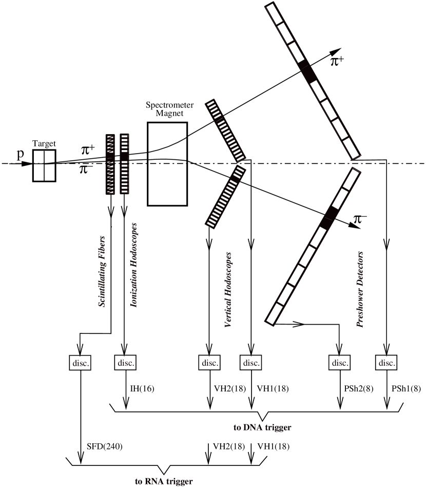
Figure 6: DIRAC detectors used for the neural network triggers DNA and RNA. Numbers of signals from each detector are given in parentheses.

DNA is able to handle the events with up to 2 hits in each vertical hodoscope VH and up to 5 hits in each IH X-plane. If the number of hits exceeds these values in any of these detectors, DNA accepts the event for further off-line evaluation. In case there is only 1 hit in an IH plane, it is assumed that two particles cross the same IH slab.

Each IH plane is used independently in combination with both VHs. Therefore DNA consists of two identical parts. Each DNA part is based on three electronic modules: the interface and decision card [10], the neural network cards [11] and the POWER-PC VME master CPU card (Motorola MVME 2302). The subdecisions of the two parts are combined in a logical OR to minimize inefficiency due to gaps between the IH slabs.

The neural network was trained to select particle pairs with low relative momenta: $Q_{x}<3\,$MeV/$c$, $Q_{y}<10\,$MeV/$c$ and $Q_{L}<30\,$MeV/$c$. The events which do not satisfy any of these conditions are considered “bad” and rejected. The training of the system was done initially with Monte-Carlo simulated events and then, before the implementation in the DIRAC trigger system, checked with real experimental data.

The DNA logic starts with T0 and in about 210 ns evaluates an event. Since DNA does not take into account any Cherenkov or horizontal hodoscopes information, an event selected by DNA is only further processed if it is also accepted by the T1 (or T1$\cdot$T2) trigger. The DNA rejection is approximately 2.3 in respect to T1. Its efficiency in the low $Q$ region is 94%.

To increase the selection efficiency, the DNA logic at the later stage of the experiment was supplemented with the RNA trigger system. The RNA operation is similar to that of DNA. Instead of the IH data, RNA uses the information from the X-plane of the scintillating fiber detector SFD. Figure 6 shows the related detectors used. Finer granularity upstream the magnet (0.5 mm in SFD in comparison with 6 mm in IH) provides higher trigger efficiency for pion pairs with small opening angles. The RNA decision time is 250 ns.

The OR between DNA and RNA provides a rate rejection of 1.9–2.0, at the same time increasing the efficiency in the low momentum $Q$ range to 99%.

8 Trigger 4

Trigger 4 is the final trigger stage. It reconstructs straight tracks in the X-projection of the drift chambers and analyses them with respect to relative momentum. T4 starts with a T1 trigger signal.

T4 includes two stages: the track finder and the track analyser. The track finder (an identical processor is used for each arm) receives the numbers of the fired wires from all drift chamber X-planes. Drift time values are not used in the T4 logic. The block diagram of the T4 operation is shown in Fig. 7.

Figure 7: T4 operation block diagram. Only the drift chamber X-planes involved in T4 are shown.

The track finder operation is based on an endpoint algorithm. Drift chamber planes X1 (or X2) and X5 (or X6) are the base planes for the track search (in total there are 6 X-planes in each spectrometer arm). Every pair of the hits in the base planes is considered as end points of a straight line. Each of allowed hit combination is used to select a pattern window for the intermediate planes. A track is assumed to be found if the number of hits within the window exceeds a preset value. The window width and position can be set for every plane independently. The minimum number of hits per track is also variable (a typically used value is 4). A unique number, “track identifier”, which contains the encoded numbers of the fired wires in the base planes, is ascribed to the found track. Parasitic combinations (i.e. repeated track identifiers) are suppressed by the track finder.

If tracks are found in both arms, the track analyser continues the event evaluation. The look-up memory of the track analyser contains all possible combinations of the track identifiers for pion pairs with $Q_{L}\leq 30\,$MeV/$c$ and $Q_{x}\leq 3\,$MeV/$c$. These “allowed” combinations are obtained with simulation using the precise geometry of the setup. The track analyser receives the track identifiers from both arms and compares them with the content of the look-up memory. If a relevant combination is found, the T4 processor generates a positive decision signal which starts the data transfer to the VME buffer memories. Otherwise, the Clear and Reset signals are applied to the DAQ and trigger systems.

T4 is able to operate in different modes which are defined by several parameters loaded at the start of the data taking run. In the standard mode:

• Presence of the positive decision of the DNA/RNA trigger at the T4 input is mandatory;

• A special “transparent” input is activated. If the signal at this input is present when T4 starts, T4 always generates a positive decision. The calibration trigger marks are sent to this input thus disabling their rejection;

• Timeout for the T4 decision is enabled. If a decision is not reached before the end of the timeout interval, a positive decision is generated unconditionally.

The T4 decision time is not fixed and depends on the complexity of the event. Being in average around 3.5 $\mu$s, it varies from less than 1.5 $\mu$s for simple events to more than 20 $\mu$s for the most complicated ones. To avoid large dead time losses (and due to some restrictions imposed by MSGC Clear process) the timeout interval is set to 10 $\mu$s.

The track finder stage provides additional rejection of 10–20% events depending on background conditions. Rejected events are ones without tracks in DC X-planes. The main part of the rate reduction comes from the track analyser. The complete T4 provides a rejection factor of around 5 with respect to the T1 rate or around 2.5 with respect to DNA/RNA. The T4 efficiency in the low $Q$ region exceeds 99%.

9 Trigger control and operation

The whole trigger system is fully computer controlled: no manual operations are needed in order to modify the trigger conditions. The developed trigger software allows one to vary the electronic logic or the front-end settings. At the beginning of the data taking phase the corresponding parameters of all electronic modules are loaded using the files which define the status of the front-end and trigger electronics in accordance with the selected trigger (thresholds, enabled trigger levels or modes, prescaling factors for different calibration triggers etc.).

The complete trigger system operates in the following way. In the first trigger version, Fig. 2a, a coincidence of the T1 and T2 triggers starts digitization in the FERA [12] modules (ADC, TDC etc.) and in the drift chamber electronics. The positive T3 and DNA decisions joined in a logical OR trigger the MSGC electronics and allow the readout of the whole event to buffer memories. When an event is rejected, the data in the FERA and DC branches are cleared and no readout takes place; no Clear is applied to MSGC as they were not started yet. The T1$\cdot$T2 signal inhibits generation of a new T1 and T0 until the end of the Clear processes followed by either readout or discarding of the data after a negative decision.

At the typical experimental conditions quoted in Sec. 1 the T1 rate is close to 5000/spill, the rate of accepted events is 1800–2000/spill (the ratio of the rates exceeds the reduction factor 1.9 of T3+DNA due to the dead time of the data acquisition and trigger systems). The calibration $e^{+}e^{-}$, $\Lambda$ and $K$ triggers (used with the prescaling factors 7, 3 and 2, respectively) constitute 15% of the accepted event sample. With these rates an overflow of the buffer memories in some readout branches occurs occasionally and the rate capability of the data acquisition system is near the limit when the setup receives several beam bunches close in time. To eliminate these drawbacks a different trigger version, Fig. 2b, is used.

In this revised trigger version the drift chamber processor T4 and the additional neural trigger chain RNA were implemented. The T2 and T3 stages were skipped as they did not add considerably to the rate or dead time reduction anymore.

In Fig. 2b digitization starts with T1. Similarly to the previous scheme, in case of the negative decision of DNA+RNA the data in the FERA and $DC$ branches are cleared. The positive DNA+RNA decision starts the MSGC electronics and gives the confirmation to T4 to begin processing.

The negative T4 decision leads to Clear of data in all branches including MSGC. Note that MSGC clearing takes more time than that in any other branch and for this reason MSGCs start later. Therefore dead time losses from the MSGC clear process occur only when T4 rejects an event already accepted by DNA+RNA. All events accepted by T4 are transferred to the VME memories to be read out for further off-line analysis.

At the same T1 rate of 5000/spill the DNA+RNA rate is 2000–2200/spill and the T4 rate of accepted events is around 700/spill. The sum of the calibration triggers is around 20% at the applied prescaling factors 14, 6 and 4 for $e^{+}e^{-}$, $\Lambda$ and $K$-triggers, respectively.

The performance of the trigger is illustrated in Figs. 8–11. In Fig. 8 the acceptance of different triggers as a function of the relative momentum $Q$ is presented. The curves for events selected by T1, T1$\cdot$(DNA+RNA), T1$\cdot$T4 and for the complete trigger T1$\cdot$(DNA+RNA)$\cdot$T4 are shown. In Figs. 9 and 10 the efficiencies of triggers are shown with respect to T1 (the ratios of the curves in Fig. 8 to the T1 curve). The efficiency for selecting low $Q$ events by the trigger processors is evident.

Figure 8: Total relative momentum $Q$ for events selected by different trigger levels.

Figure 9: Efficiency of DNA+RNA, T4 and (DNA+RNA)$\cdot$T4 triggers with respect to T1 as a function of total $Q$.

Figure 10: Same as in Fig. 9 with an expanded $Q$ scale.

Figure 11: Efficiency of DNA+RNA, T4 and (DNA+RNA)$\cdot$T4 triggers with respect to T1 as a function of $Q_{L}$ for events with $Q_{x}<3\,$MeV/$c$ and $Q_{y}<3\,$MeV/$c$.

The efficiencies of triggers as a function of the longitudinal component of the relative momentum, $Q_{L}$, when $Q_{x}<3\,$MeV/$c$ and $Q_{y}<3\,$MeV/$c$ are presented in Fig.9. The T4 efficiency alone with respect to T1 is over 99% in the whole region $|Q_{L}|<30\,$MeV/$c$. Common selection by DNA+RNA and T4 results in the 98% efficiency for $|Q_{L}|<22\,$MeV/$c$ and 95% for $|Q_{L}|<30\,$MeV/$c$.

The complete trigger provides a factor of 1000 in rate reduction with respect to the single counting rates of the downstream detectors keeping a high efficiency in the range of low pair relative momenta.

10 Trigger quality control

Improper trigger functioning could lead to losses of events or systematic biases in the collected data which cannot be corrected later at the off-line analysis. For that reason the trigger quality is under permanent control.

The counting rates of different triggers and their submodes at all trigger levels are measured by CAMAC scalers. Their content is read out and recorded at the end of every accelerator spill and is also displayed by the on-line monitoring program. This provides control over the trigger stability.

The trigger efficiency is under control as well. One of the TDC modules (the “trigger register”) is intended for detection of trigger marks. Each decision of every trigger level, its submode type and arrival time per event are recorded. This information is available for the off-line analysis and on-line monitoring.

To test the efficiency of all higher than T1 triggers, their rejection power and acceptance in terms of the relative momentum $Q$, data are periodically collected with T1 as the only active trigger. The other triggers perform their analysis and send their trigger marks to the trigger register (T4 decisions, due to its longer processing time, are written in a special “mail box” in the DC buffer memory). A regular off-line express-analysis permits the detection of any deviations in the trigger performance. The results presented in Figs. 8–11 were obtained just from such data collected with T1 trigger.

To check the operation of the whole trigger system, including the primary T1 and T0 steps, a special minimum bias trigger is sometimes used. Two minimum bias trigger options are available with the simplest logic: IH$\cdot$VH1 or IH$\cdot$VH2, i.e. with only one upstream and one downstream detector involved. The events thus triggered may contain hits in other detectors as well and eventually even other trigger processors may select them. In these cases all the corresponding trigger marks should be generated. Off-line analysis of the data from all the detectors together with the recorded trigger marks makes it possible to test the trigger efficiency at all trigger stages.

One more trigger is arranged for tests of the front-end, trigger and readout electronics. Artificially generated signals are sent to inputs of the front-end electronics of all the detectors (except SFD, MSGC and DC). Relative delays between the generator signals coming to different detector groups are adjusted to be like those from real particles. As a result, all electronic channels in the trigger and readout modules can be tested.

11 Conclusions

The trigger system of DIRAC has been operating since 1999. It passed through several upgrade steps and at present provides considerable trigger rate reduction which satisfies the rate capabilities of the data acquisition system and the volume of the buffer memories used. The system proved to be reliable and convenient for the users.

References

- [1] B.Adeva et al.: Lifetime measurement of atoms to test low energy QCD predictions, Proposal to the SPSLC, CERN/SPSLC 95-1, SPSLC/P 284, December 1994.
- [2] L.Afanasyev, M.Gallas, V.Karpukhin, A.Kulikov, NIM, A479 (2002) 407–411.
- [3] F.Takeutchi: Study of the trigger logic with front-end detectors II, Report at the DIRAC trigger/electronics meeting, CERN, February 1996.
- [4] V.Agoritsas et al., NIM A411 (1998) 17–30.
- [5] A.Gorin et al., NIM A452 (2000) 280–288.
- [6] V.Karpukhin, A.Kulikov, V.Yazkov: Third level trigger for DIRAC. Versions of implementation, DIRAC Note 96-27, CERN, 1996.
-
[7]
M.Gallas: The Complete Software-Programmable
Third Level Trigger for DIRAC,
Application Note AN-60, LeCroy Corporation, 1999.
M.Gallas: Third level trigger of the DIRAC experiment, To be published in NIM A482/1-2. - [8] P.Kokkas, M.Steinacher, L.Tauscher, S.Vlachos, NIM A471 (2001) 358–367.
- [9] F.R.Leimgruber et al., NIM A365 (1995) 198–202.
- [10] M.Steinacher: Interface and decision card; the design, Revision 2.0, Internal Report, University of Basel, 1999.
- [11] M.Steinacher: Hardware implementation of a fast neural network, In Proceedings of the Sixth International Workshop on Software Engineering, Artificial Intelligence and Expert Systems (AIENP 1999), Parisianou Press, Heraclion, 2000.
- [12] Fast Encoding and Readout ADC System Possibilities, Application Note AN-4004A, LeCroy Corporation.