G. Calderini
Stanford Linear Accelerator Center
2575 Sand Hill rd. Menlo Park, CA 94025
(for the B AB AR Collaboration)

Using 22.7 million $B\overline{B}$ events recorded with the BABAR detector, the inclusive branching fractions for the production of $J/\psi$, $\psi(2S)$ and $\chi_{c}$ in $B$ decays are presented. Combining the charmonium state with a $K^{\pm}$, $K^{0}$, $K^{*\pm}$, $K^{*0}$ or $\pi^{0}$, $B$ decays are reconstructed exlusively and branching fractions are determined. A preliminary study is also presented for the $B\rightarrow\eta_{c}K$ decay mode.

Contributed to the Proceedings of HEP2001

International Europhysics Conference on High Energy Physics,

7/12/2001—7/18/2001, Budapest, Hungary

1 Introduction

Reconstruction and study of charmonium mesons in $B$ decays is a crucial component of the measurement of time-dependent CP-violating asymmetries[1].

The analyses described in the following paper are based on a sample of 20.7 fb^-1 collected with BABAR at the $\mathchar 28935\relax(4S)~{}$resonance with an additional 2.6 fb^-1 collected below the $B\overline{B}~{}$threshold. A determination of the $B$ meson branching fractions depends upon an accurate measurement of the number of $B$ mesons in the data sample. The number of $B\overline{B}~{}$events is determined by comparing the rate of multi-hadron events in data collected both on and off resonance. The continuum contribution to the on-resonance sample is estimated by rescaling the number of off-resonance hadronic events by the ratio of the number of observed $\mu^{+}\mu^{-}$ events in the two samples. This procedure yields a total of $22.72\pm 0.36$ million $B\overline{B}~{}$events.

2 Inclusive decays of $B$ to states containing Charmonium

${J\mskip-3.0mu/\mskip-2.0mu\psi\mskip 2.0mu}$ candidates are selected by requiring two identified leptons of opposite charge. Electrons are identified based on the ratio $E/p$ of the energy deposited in the calorimeter to the measured momentum from tracking information, the shape of the calorimetric cluster and the ionization in the tracking detectors. Muons are identified by requiring a minimum ionizing signal in the calorimeter. In addition, the shape and penetration of the distribution of hits in the instrumented flux return are used. The number of ${J\mskip-3.0mu/\mskip-2.0mu\psi\mskip 2.0mu}$ events is determined by fitting the invariant mass distribution to a probability density function obtained from a simulation including contribution from both final state radiation and bremsstrahlung. The fit yields $15739\pm 177$ ${J\mskip-3.0mu/\mskip-2.0mu\psi\mskip 2.0mu}$ $\rightarrow e^{+}e^{-}$ and $13683\pm 154$ ${J\mskip-3.0mu/\mskip-2.0mu\psi\mskip 2.0mu}$ $\rightarrow\mu^{+}\mu^{-}$ signal events (Figure 1).

Figure 1: Invariant mass distributions for inclusive $J/\psi$ production in $B$ decays

The $\psi(2S)~{}$candidates are reconstructed in the $\psi(2S)~{}$$\rightarrow l^{+}l^{-}$ and $\psi(2S)~{}$$\rightarrow J/\psi\pi^{+}\pi^{-}$ decays. In the latter case the signal yield is extracted by a fit to the mass difference between the $\psi(2S)~{}$and the ${J\mskip-3.0mu/\mskip-2.0mu\psi\mskip 2.0mu}$ reconstructed candidates. We find $552\pm 50$ decays to $e^{-}e^{-}$, $437\pm 44$ decays to $\mu^{+}\mu^{-}$, $405\pm 37$ decays to $J/\psi(e^{+}e^{-})\pi^{+}\pi^{-}$ and $400\pm 34$ decays to $J/\psi(\mu^{+}\mu^{-})\pi^{+}\pi^{-}$.

The $\chi_{c1}~{}$and $\chi_{c2}~{}$candidates are selected by combining a reconstructed ${J\mskip-3.0mu/\mskip-2.0mu\psi\mskip 2.0mu}$ with a photon. The signal yield is determined by fitting the mass difference between the $\chi_{c~{}}$ and the ${J\mskip-3.0mu/\mskip-2.0mu\psi\mskip 2.0mu}$ candidates. The shape of the signal is extracted from Monte Carlo, with the mass difference between the $\chi_{c1}~{}$and $\chi_{c2}~{}$peaks fixed to the PDG value [2]. The fit gives $476\pm 71$ $\chi_{c1}~{}$and $86\pm 59$ $\chi_{c2}~{}$candidates for the $J/\psi\rightarrow e^{+}e^{-}$ decay and $545\pm 60$ $\chi_{c1}~{}$and $104\pm 56$ $\chi_{c2}~{}$candidates for the $J/\psi\rightarrow\mu^{+}\mu^{-}$ decay.

Mode	Br($\times 10^{-2}$)
$B\rightarrow J/\psi~{}X$	$1.044\pm 0.013\pm 0.028$
$B\rightarrow\psi(2s)~{}X$	$0.275\pm 0.020\pm 0.029$
$B\rightarrow\chi_{c1}X$	$0.378\pm 0.034\pm 0.026$
$B\rightarrow\chi_{c2}X$	$<0.21~{}(90\%~{}CL)$

Table 1: Measured branching fractions for inclusive charmonium production in $B$ decays.

Values for the branching fractions are extracted from the yields[3]. A $90\%$ CL limit is set on the $B$ decay to $\chi_{c2}~{}$. The results for the inclusive production of ${J\mskip-3.0mu/\mskip-2.0mu\psi\mskip 2.0mu}$, $\psi(2S)~{}$and $\chi_{c~{}}$ in $B$ decays are summarized in Table 1, where the first uncertainty is statistical error and the second is systematics.

3 Exclusive decays of $B$ to Charmonium

The reconstruction of exclusive decay modes containing charmonium presents a very low background in most of the channels. For this reason the lepton identification criteria are loosened for one of the two ${J\mskip-3.0mu/\mskip-2.0mu\psi\mskip 2.0mu}$ decay products. As in the inclusive analysis, $\psi(2S)~{}$candidates are reconstructed by their decay to $e^{-}e^{-}$, $\mu^{+}\mu^{-}$ and $J/\psi~{}\pi^{+}\pi^{-}$. The $\chi_{c~{}}$ candidates are selected through their decay to $J/\psi\gamma$.

The charmonium states are selected in a window around their expected mass[2] for the decays to leptons. In the decays to ${J\mskip-3.0mu/\mskip-2.0mu\psi\mskip 2.0mu}$ states the mass difference distribution between the charmonium candidate and the reconstructed ${J\mskip-3.0mu/\mskip-2.0mu\psi\mskip 2.0mu}$ is used instead.

Selected candidates are then paired with a $K^{+}$, $K_{s}^{0}~{}$(either $\pi^{+}\pi^{-}~{}$or $\pi^{0}\pi^{0}~{}$), $K^{*+}$ (either $K^{+}$$\pi^{0}$ or $K_{s}^{0}~{}$$\pi^{+}$), $K^{*0}~{}$(either $K^{+}\pi^{-}$ or $K_{s}^{0}~{}$$\pi^{0}$), $\pi^{0}$ or $K_{L}$ to form a $B$ candidate. The two most significant observables used to identify the signal are the difference $\Delta E~{}$in the center-of-mass frame between the reconstructed $B$ energy and half the nominally available energy, $\sqrt{s}/2$, and the energy-substituted mass, $m_{ES}=\sqrt{s/4-{P_{B}^{*2}}}$, where $P_{B}^{*}$ is the center-of-mass momentum of the $B$ candidate. A sample of these distributions is given in Figure 2 for $J/\psi K_{S}$ events.

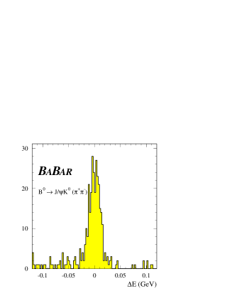
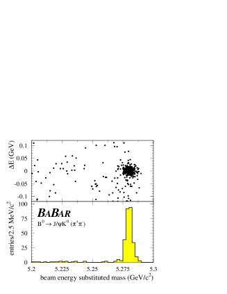
Figure 2: Example of the $\Delta E~{}$(left) and $m_{ES}$ (right) distributions for the decay $B^{0}\rightarrow J/\psi K_{s}^{0}$

In the case of multiple candidates per event, only the candidate with the smallest $|\Delta E|$ is selected. For all modes except $B\rightarrow J/\psi K_{L}$ and $B\rightarrow J/\psi K^{*}$, the number of signal events is determined from the observed number of events in the $(\Delta E,m_{ES})$ region after background subtraction. In addition to the usual combinatorial component, the background distribution shows an excess of events in the signal region. The combinatorial contribution is estimated by using an ARGUS function in the fit to the $m_{ES}$ distribution. The peaking background component is obtained from simulation of inclusive $B$ decays to charmonium, after removing the signal events.

The signal yields for the $K^{*0}$ and $K^{*+}$ modes are determined simultaneously from a likelihood fit, which is needed to account for the cross-feed between the $K^{*}$ decay channels.

A different technique is used for the $B\rightarrow J/\psi K_{L}$ decay mode. In this case only the $K_{L}$ direction is measured with information from the calorimeter and the instrumented flux return. Given this direction and the reconstructed charmonium candidate, the $K_{L}$ energy is extracted by using the $B$ mass as a constraint. To eliminate cross-feed from other decay modes, a veto has been introduced for events which have been selected already in other exclusive modes. This procedure yields a purity of about $50\%$. Due to this method, the $m_{ES}$ distribution cannot be used to determine the signal yield. The $\Delta E_{J/\psi K^{0}_{L}}$ distribution is used in a log-likelihood fit. The shapes of the signal and inclusive charmonium background components are taken from Monte Carlo simulations. The shape of the non-charmonium background component is taken from an ARGUS fit to the $\Delta E_{K^{0}_{L}}$ distribution for events in the ${J\mskip-3.0mu/\mskip-2.0mu\psi\mskip 2.0mu}$ mass sideband. After the background subtraction, this channel gives a signal yield of $183\pm 14$ events (Figure 3, left plot).

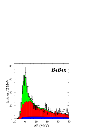
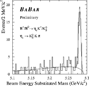
Figure 3: (Left plot) $\Delta E~{}$distribution for $B^{0}\rightarrow J/\psi K_{L}$ decays. Points are data, solid line is the Monte Carlo simulation. The three components are respectively signal, background events which include a real $J/\psi$, and non-$J/\psi$ background. (Right plot) preliminary study of $B$ decay to $\eta_{c}K$. In the above plot the $\eta_{c}$ candidate is reconstructed through $K_{S}K\pi$ decays.

Mode		Yield	Br($\times 10^{-4}$)
$B^{0}\rightarrow J/\psi K^{0}$	$K_{S}^{0}\rightarrow\pi^{+}\pi^{-}$	$265.5\pm 2.9$	$8.5\pm 0.5\pm 0.6$
	$K_{S}^{0}\rightarrow\pi^{0}\pi^{0}$	$62.5\pm 3.8$	$9.6\pm 1.5\pm 0.7$
	$K_{L}^{0}$	$183\pm 14$	$6.8\pm 0.8\pm 0.8$
	All		$8.3\pm 0.4\pm 0.5$
$B^{+}\rightarrow J/\psi K^{+}$		$1109\pm 4$	$10.1\pm 0.3\pm 0.5$
$B^{0}\rightarrow J/\psi\pi^{0}$		$13.6\pm 0.9$	$0.20\pm 0.06\pm 0.02$
$B^{0}\rightarrow J/\psi K^{*0}$		$594\pm 8.5$	$12.4\pm 0.5\pm 0.9$
$B^{+}\rightarrow J/\psi K^{*+}$		$377.4\pm 16.9$	$13.7\pm 0.9\pm 1.1$
$B^{0}\rightarrow\psi(2S)K^{0}$		$56.0\pm 3.4$	$6.8\pm 1.0\pm 1.1$
$B^{+}\rightarrow\psi(2S)K^{+}$		$207.3\pm 6.2$	$6.3\pm 0.5\pm 0.8$
$B^{0}\rightarrow\chi_{c1}K^{0}$		$26.1\pm 2.5$	$5.4\pm 1.4\pm 1.1$
$B^{+}\rightarrow\chi_{c1}K^{+}$		$145.1\pm 7.2$	$7.5\pm 0.8\pm 0.8$
$B^{0}\rightarrow\chi_{c1}K^{*0}$		$32.6\pm 6.0$	$4.8\pm 1.4\pm 0.9$
$B^{0}\rightarrow J/\psi\pi^{+}\pi^{-}$		$29.1\pm 9.4$	$0.46\pm 0.11\pm 0.08$

Table 2: Summary of the signal yields and extracted branching fractions for the different $B$ decays reconstructed into exclusive charmonium final states by the BABAR analyses described in this paper.

The information on the signal yields and the measured branching fractions for all presented exclusive modes[4] is summarized in Table 2, while Figure 4 shows a comparison of the new preliminary BABAR results to the current PDG values.

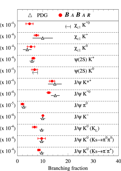
Figure 4: Comparison of the preliminary results from the BABAR summarized in the previous table and the published PDG values.

In addition to the analyses described above, a very preliminary study has been recently performed by BABAR, on exclusive reconstruction of $B$ decays to $\eta_{c}K$ modes. The $\eta_{c}$ has been studied in the $K_{S}K^{+}\pi^{-}$, $K^{+}K^{-}\pi^{0}$ and $K^{+}K^{-}K^{+}K^{-}$ ($\phi\phi$ plus non-resonant) decay modes. The energy-substituted mass distribution for the decay $\eta_{c}\rightarrow K_{S}K^{+}\pi^{-}$ is presented as an example in Figure 3, right plot. No value has been extracted yet for the branching fractions in these decay modes.

4 Summary

Using 22.7 million $B\overline{B}~{}$events recorded by the BABAR detector, the inclusive branching fractions for the production of ${J\mskip-3.0mu/\mskip-2.0mu\psi\mskip 2.0mu}$, $\psi(2S)~{}$and $\chi_{c~{}}$ are presented. Combining the charmonium state with either a $K^{\pm}~{}$, $K^{0}$, $K^{*\pm}~{}$, $K^{*0}~{}$or $\pi^{0}$, $B$ decays are reconstructed exclusively and their branching fractions are determined.

References

- [1] BaBar Collaboration, “Observation of CP-violation in the meson system”, Phys.Rev.Lett. 87, 091801 (2001).
- [2] Particle Data Group, D.E. Groom et al., Eur. Phys. Jour. C 15(2000)1.
- [3] BaBar Collaboration, “Measurement of inclusive production of charmonium states in meson decays”, BABAR-CONF-00/04, hep-ex/0008049
- [4] BaBar Collaboration, “Measurement of branching fractions for exclusive decays to charmonium final states”, BABAR-PUB-01/07, hep-ex/0107025