EUROPEAN ORGANIZATION FOR NUCLEAR RESEARCH

CERN-EP-2002-014

15 February 2002

Measurement of the Hadronic
Photon Structure Function $F_{2}^{\gamma}$
at LEP2

The OPAL Collaboration

The hadronic structure function of the photon $F_{2}^{\gamma}(x,Q^{2})$ is measured as a function of Bjorken $x$ and of the photon virtuality $Q^{2}$ using deep-inelastic scattering data taken by the OPAL detector at LEP at $\mathrm{e}^{+}\mathrm{e}^{-}$ centre-of-mass energies from 183 to 209 GeV. Previous OPAL measurements of the $x$ dependence of $F_{2}^{\gamma}$ are extended to an average $Q^{2}$ of $\langle Q^{2}\rangle=780$ $\mathrm{GeV}^{2}$ using data in the kinematic range $0.15<x<0.98$. The $Q^{2}$ evolution of $F_{2}^{\gamma}$ is studied for $12.1<\langle Q^{2}\rangle<780$ $\mathrm{GeV}^{2}$ using three ranges of $x$. As predicted by QCD, the data show positive scaling violations in $F_{2}^{\gamma}$ with $F_{2}^{\gamma}(Q^{2})/\alpha=(0.08\,\pm 0.02\,^{+\,0.05}_{-\,0.03})+(0.13\,\pm 0.01\,^{+\,0.01}_{-\,0.01})\,\ln\,Q^{2}$, where $Q^{2}$ is in $\mathrm{GeV}^{2}$, for the central $x$ region 0.10–0.60. Several parameterisations of $F_{2}^{\gamma}$ are in qualitative agreement with the measurements whereas the quark-parton model prediction fails to describe the data.

(Submitted to Physics Letters B)

The OPAL Collaboration

G. Abbiendi², C. Ainsley⁵, P.F. Åkesson³, G. Alexander²², J. Allison¹⁶, G. Anagnostou¹, K.J. Anderson⁹, S. Asai²³, D. Axen²⁷, G. Azuelos^18,a, I. Bailey²⁶, E. Barberio⁸, R.J. Barlow¹⁶, R.J. Batley⁵, P. Bechtle²⁵, T. Behnke²⁵, K.W. Bell²⁰, P.J. Bell¹, G. Bella²², A. Bellerive⁶, G. Benelli⁴, S. Bethke³², O. Biebel³², I.J. Bloodworth¹, O. Boeriu¹⁰, P. Bock¹¹, D. Bonacorsi², M. Boutemeur³¹, S. Braibant⁸, L. Brigliadori², R.M. Brown²⁰, K. Buesser²⁵, H.J. Burckhart⁸, J. Cammin³, S. Campana⁴, R.K. Carnegie⁶, B. Caron²⁸, A.A. Carter¹³, J.R. Carter⁵, C.Y. Chang¹⁷, D.G. Charlton^1,b, I. Cohen²², A. Csilling^8,g, M. Cuffiani², S. Dado²¹, G.M. Dallavalle², S. Dallison¹⁶, A. De Roeck⁸, E.A. De Wolf⁸, K. Desch²⁵, M. Donkers⁶, J. Dubbert³¹, E. Duchovni²⁴, G. Duckeck³¹, I.P. Duerdoth¹⁶, E. Etzion²², F. Fabbri², L. Feld¹⁰, P. Ferrari¹², F. Fiedler⁸, I. Fleck¹⁰, M. Ford⁵, A. Frey⁸, A. Fürtjes⁸, P. Gagnon¹², J.W. Gary⁴, G. Gaycken²⁵, C. Geich-Gimbel³, G. Giacomelli², P. Giacomelli², M. Giunta⁴, J. Goldberg²¹, E. Gross²⁴, J. Grunhaus²², M. Gruwé⁸, P.O. Günther³, A. Gupta⁹, C. Hajdu²⁹, M. Hamann²⁵, G.G. Hanson¹², K. Harder²⁵, A. Harel²¹, M. Harin-Dirac⁴, M. Hauschild⁸, J. Hauschildt²⁵, C.M. Hawkes¹, R. Hawkings⁸, R.J. Hemingway⁶, C. Hensel²⁵, G. Herten¹⁰, R.D. Heuer²⁵, J.C. Hill⁵, K. Hoffman⁹, R.J. Homer¹, D. Horváth^29,c, R. Howard²⁷, P. Hüntemeyer²⁵, P. Igo-Kemenes¹¹, K. Ishii²³, H. Jeremie¹⁸, C.R. Jones⁵, P. Jovanovic¹, T.R. Junk⁶, N. Kanaya²⁶, J. Kanzaki²³, G. Karapetian¹⁸, D. Karlen⁶, V. Kartvelishvili¹⁶, K. Kawagoe²³, T. Kawamoto²³, R.K. Keeler²⁶, R.G. Kellogg¹⁷, B.W. Kennedy²⁰, D.H. Kim¹⁹, K. Klein¹¹, A. Klier²⁴, S. Kluth³², T. Kobayashi²³, M. Kobel³, T.P. Kokott³, S. Komamiya²³, L. Kormos²⁶, R.V. Kowalewski²⁶, T. Krämer²⁵, T. Kress⁴, P. Krieger^6,l, J. von Krogh¹¹, D. Krop¹², T. Kuhl²⁵, M. Kupper²⁴, P. Kyberd¹³, G.D. Lafferty¹⁶, H. Landsman²¹, D. Lanske¹⁴, J.G. Layter⁴, A. Leins³¹, D. Lellouch²⁴, J. Letts¹², L. Levinson²⁴, J. Lillich¹⁰, C. Littlewood⁵, S.L. Lloyd¹³, F.K. Loebinger¹⁶, J. Lu²⁷, J. Ludwig¹⁰, A. Macchiolo¹⁸, A. Macpherson^28,i, W. Mader³, S. Marcellini², T.E. Marchant¹⁶, A.J. Martin¹³, J.P. Martin¹⁸, G. Masetti², T. Mashimo²³, P. Mättig²⁴, W.J. McDonald²⁸, J. McKenna²⁷, T.J. McMahon¹, R.A. McPherson²⁶, F. Meijers⁸, P. Mendez-Lorenzo³¹, W. Menges²⁵, F.S. Merritt⁹, H. Mes^6,a, A. Michelini², S. Mihara²³, G. Mikenberg²⁴, D.J. Miller¹⁵, S. Moed²¹, W. Mohr¹⁰, T. Mori²³, A. Mutter¹⁰, K. Nagai¹³, I. Nakamura²³, H.A. Neal³³, R. Nisius⁸, S.W. O’Neale¹, A. Oh⁸, A. Okpara¹¹, M.J. Oreglia⁹, S. Orito²³, C. Pahl³², G. Pásztor^8,g, J.R. Pater¹⁶, G.N. Patrick²⁰, J.E. Pilcher⁹, J. Pinfold²⁸, D.E. Plane⁸, B. Poli², J. Polok⁸, O. Pooth⁸, A. Quadt³, K. Rabbertz⁸, C. Rembser⁸, P. Renkel²⁴, H. Rick⁴, J.M. Roney²⁶, S. Rosati³, Y. Rozen²¹, K. Runge¹⁰, D.R. Rust¹², K. Sachs⁶, T. Saeki²³, O. Sahr³¹, E.K.G. Sarkisyan^8,j, A.D. Schaile³¹, O. Schaile³¹, P. Scharff-Hansen⁸, M. Schröder⁸, M. Schumacher³, C. Schwick⁸, W.G. Scott²⁰, R. Seuster^14,f, T.G. Shears^8,h, B.C. Shen⁴, C.H. Shepherd-Themistocleous⁵, P. Sherwood¹⁵, G. Siroli², A. Skuja¹⁷, A.M. Smith⁸, R. Sobie²⁶, S. Söldner-Rembold^10,d, S. Spagnolo²⁰, F. Spano⁹, A. Stahl³, K. Stephens¹⁶, D. Strom¹⁹, R. Ströhmer³¹, S. Tarem²¹, M. Tasevsky⁸, R.J. Taylor¹⁵, R. Teuscher⁹, M.A. Thomson⁵, E. Torrence¹⁹, D. Toya²³, P. Tran⁴, T. Trefzger³¹, A. Tricoli², I. Trigger⁸, Z. Trócsányi^30,e, E. Tsur²², M.F. Turner-Watson¹, I. Ueda²³, B. Ujvári^30,e, B. Vachon²⁶, C.F. Vollmer³¹, P. Vannerem¹⁰, M. Verzocchi¹⁷, H. Voss⁸, J. Vossebeld⁸, D. Waller⁶, C.P. Ward⁵, D.R. Ward⁵, P.M. Watkins¹, A.T. Watson¹, N.K. Watson¹, P.S. Wells⁸, T. Wengler⁸, N. Wermes³, D. Wetterling¹¹ G.W. Wilson^16,k, J.A. Wilson¹, T.R. Wyatt¹⁶, S. Yamashita²³, V. Zacek¹⁸, D. Zer-Zion⁴

¹School of Physics and Astronomy, University of Birmingham, Birmingham B15 2TT, UK
²Dipartimento di Fisica dell’ Università di Bologna and INFN, I-40126 Bologna, Italy
³Physikalisches Institut, Universität Bonn, D-53115 Bonn, Germany
⁴Department of Physics, University of California, Riverside CA 92521, USA
⁵Cavendish Laboratory, Cambridge CB3 0HE, UK
⁶Ottawa-Carleton Institute for Physics, Department of Physics, Carleton University, Ottawa, Ontario K1S 5B6, Canada
⁸CERN, European Organisation for Nuclear Research, CH-1211 Geneva 23, Switzerland
⁹Enrico Fermi Institute and Department of Physics, University of Chicago, Chicago IL 60637, USA
¹⁰Fakultät für Physik, Albert Ludwigs Universität, D-79104 Freiburg, Germany
¹¹Physikalisches Institut, Universität Heidelberg, D-69120 Heidelberg, Germany
¹²Indiana University, Department of Physics, Swain Hall West 117, Bloomington IN 47405, USA
¹³Queen Mary and Westfield College, University of London, London E1 4NS, UK
¹⁴Technische Hochschule Aachen, III Physikalisches Institut, Sommerfeldstrasse 26-28, D-52056 Aachen, Germany
¹⁵University College London, London WC1E 6BT, UK
¹⁶Department of Physics, Schuster Laboratory, The University, Manchester M13 9PL, UK
¹⁷Department of Physics, University of Maryland, College Park, MD 20742, USA
¹⁸Laboratoire de Physique Nucléaire, Université de Montréal, Montréal, Quebec H3C 3J7, Canada
¹⁹University of Oregon, Department of Physics, Eugene OR 97403, USA
²⁰CLRC Rutherford Appleton Laboratory, Chilton, Didcot, Oxfordshire OX11 0QX, UK
²¹Department of Physics, Technion-Israel Institute of Technology, Haifa 32000, Israel
²²Department of Physics and Astronomy, Tel Aviv University, Tel Aviv 69978, Israel
²³International Centre for Elementary Particle Physics and Department of Physics, University of Tokyo, Tokyo 113-0033, and Kobe University, Kobe 657-8501, Japan
²⁴Particle Physics Department, Weizmann Institute of Science, Rehovot 76100, Israel
²⁵Universität Hamburg/DESY, II Institut für Experimental Physik, Notkestrasse 85, D-22607 Hamburg, Germany
²⁶University of Victoria, Department of Physics, P O Box 3055, Victoria BC V8W 3P6, Canada
²⁷University of British Columbia, Department of Physics, Vancouver BC V6T 1Z1, Canada
²⁸University of Alberta, Department of Physics, Edmonton AB T6G 2J1, Canada
²⁹Research Institute for Particle and Nuclear Physics, H-1525 Budapest, P O Box 49, Hungary
³⁰Institute of Nuclear Research, H-4001 Debrecen, P O Box 51, Hungary
³¹Ludwig-Maximilians-Universität München, Sektion Physik, Am Coulombwall 1, D-85748 Garching, Germany
³²Max-Planck-Institute für Physik, Föhring Ring 6, 80805 München, Germany
³³Yale University,Department of Physics,New Haven, CT 06520, USA

^a and at TRIUMF, Vancouver, Canada V6T 2A3
^b and Royal Society University Research Fellow
^c and Institute of Nuclear Research, Debrecen, Hungary
^d and Heisenberg Fellow
^e and Department of Experimental Physics, Lajos Kossuth University, Debrecen, Hungary
^f and MPI München
^g and Research Institute for Particle and Nuclear Physics, Budapest, Hungary
^h now at University of Liverpool, Dept of Physics, Liverpool L69 3BX, UK
ⁱ and CERN, EP Div, 1211 Geneva 23
^j and Universitaire Instelling Antwerpen, Physics Department, B-2610 Antwerpen, Belgium
^k now at University of Kansas, Dept of Physics and Astronomy, Lawrence, KS 66045, USA
^l now at University of Toronto, Dept of Physics, Toronto, Canada

1 Introduction

Much of the present knowledge of the structure of the photon has been obtained from measurements of the photon structure function $F_{2}^{\gamma}$ in deep-inelastic electron-photon scattering at $\mathrm{e}^{+}\mathrm{e}^{-}$ colliders, see [1] for a recent review. The large statistics and high electron energies of the full LEP2 programme permit the extension of the measurement of $F_{2}^{\gamma}$ to higher values of $\langle Q^{2}\rangle$ than have been probed at LEP1. The photon structure function $F_{2}^{\gamma}$ is expected to increase only logarithmically with $Q^{2}$ [2]. Therefore, the large range of $Q^{2}$ values accessible at LEP, which extends from about 1 $\mathrm{GeV}^{2}$ to several thousand $\mathrm{GeV}^{2}$, makes it an ideal place to study the evolution.

The measurement of $F_{2}^{\gamma}$ in $\mathrm{e}^{+}\mathrm{e}^{-}$ interactions is based on the deep-inelastic electron-photon scattering reaction, ${\rm e}(k)\,\gamma(p)\rightarrow{\rm e}(k^{\prime})\,+\,\mbox{hadrons}$, proceeding via the exchange of a virtual photon, $\gamma^{*}(q)$, where the symbols in brackets denote the four-momentum vectors of the particles. The flux of quasi-real photons can be calculated using the equivalent photon approximation [3]. The cross-section for deep inelastic electron-photon scattering is expressed as:

$$\frac{{\rm d}^{2}\sigma_{\rm e\gamma\rightarrow{\rm eX}}}{{\rm d}x{\rm d}Q^{2}}=\frac{2\pi\alpha^{2}}{x\,Q^{4}}\left[\left(1+(1-y)^{2}\right)F_{2}^{\gamma}(x,Q^{2})-y^{2}F_{\mathrm{L}}^{\gamma}(x,Q^{2})\right]$$ (1)

where $Q^{2}=-q^{2}$. The usual dimensionless variables of deep inelastic scattering, $x$ and $y$, are defined as $x=Q^{2}/2(p\cdot q)$ and $y=(p\cdot q)/(p\cdot k)$, and $\alpha$ is the fine structure constant. The structure function $F_{2}^{\gamma}$ is related to the charge-weighted sum of the parton densities of the photon (see e.g. [1]). In the kinematic region of low values of $y$ studied ($y^{2}\ll 1$) the contribution of the term proportional to the longitudinal structure function $F_{\mathrm{L}}^{\gamma}(x,Q^{2})$ is negligible [1].

The analysis presented here is based on 632 $\mathrm{pb}^{-1}$ of data at $\mathrm{e}^{+}\mathrm{e}^{-}$ centre-of-mass energies $\sqrt{s_{\rm ee}}$ of 183 to 209 GeV, with a luminosity weighted average of $\sqrt{s_{\rm ee}}=197.1$ GeV, taken by the OPAL experiment in the years 1997–2000. It extends the measurements of $F_{2}^{\gamma}$ as a function of $x$ up to $\langle Q^{2}\rangle=780$ $\mathrm{GeV}^{2}$, and significantly improves on the precision of the measurement of the $Q^{2}$ evolution of $F_{2}^{\gamma}$. This analysis not only tests perturbative QCD but also measures $F_{2}^{\gamma}$ at large $Q^{2}$, a previously unexplored region in $\mathrm{e}^{+}\mathrm{e}^{-}$ collisions. This is approximately the region which has also been probed in jet production at HERA [4, 5].

The paper is organised as follows. After the description of the OPAL detector in Section 2 the data selection is detailed in Section 3, followed by the description of the Monte Carlo simulation and background estimates in Section 4. The results are presented in Section 5. These comprise: the quality of the description of the observed hadronic final state by the Monte Carlo models, Section 5.1; the measurement of $F_{2}^{\gamma}$ at high $Q^{2}$, Section 5.2; and the measurement of the $Q^{2}$ evolution of $F_{2}^{\gamma}$, Section 5.3. Conclusions are given in Section 6.

2 The OPAL detector

A detailed description of the OPAL detector can be found in [6], and therefore only a brief account of the main features relevant to the present analysis will be given here.

The central tracking system is located inside a solenoidal magnet which provides a uniform axial magnetic field of 0.435 T along the beam axis. The magnet is surrounded by a lead-glass electromagnetic calorimeter (ECAL) and a hadronic sampling calorimeter (HCAL). Outside the HCAL, the detector is surrounded by muon chambers. There are similar layers of detectors in the endcaps. The region around the beam pipe on both sides of the detector is covered by the forward calorimeters and the silicon-tungsten luminometers.

Starting with the innermost components, the tracking system consists of a high precision silicon microvertex detector [7], a precision vertex drift chamber, a large-volume jet chamber with 159 layers of axial anode wires, and a set of $z$ chambers used to improve the measurement of the track coordinates along the beam direction. The transverse momenta $p_{\mathrm{t}}$ of tracks with respect to the $z$ direction of the detector are measured with a precision of $\sigma_{p_{\mathrm{t}}}/p_{\mathrm{t}}=\sqrt{0.02^{2}+(0.0015\cdot p_{\mathrm{t}})^{2}}$ ($p_{\mathrm{t}}$ in GeV) in the central region, $\theta>753$ mrad. The jet chamber also provides energy loss, ${\mathrm{d}}E/{\mathrm{d}}x$, measurements which are used for particle identification.

The ECAL covers the complete azimuthal range for polar angles that satisfy $\theta>200$ mrad. The barrel section, which covers the range $\theta>609$ mrad, consists of a cylindrical array of 9440 lead-glass blocks with a depth of $24.6$ radiation lengths. The endcap sections (EE) consist of 1132 lead-glass blocks with a depth of more than $22$ radiation lengths, covering angles in the range $200<\theta<609$ mrad. The electromagnetic energy resolution of the EE calorimeter is about $15\%/\sqrt{E}$ ($E$ in GeV) at polar angles above 350 mrad, but deteriorates closer to the edge of the detector.

The forward calorimeters (FD) at each end of the OPAL detector consist of cylindrical lead-scintillator calorimeters with a depth of 24 radiation lengths divided azimuthally into 16 segments. The electromagnetic energy resolution of the FD calorimeter is about $18\%/\sqrt{E}$ ($E$ in GeV). The clear acceptance of the forward calorimeters covers the range $60<\theta<140$ mrad. Three planes of proportional tube chambers at 4 radiation lengths depth in the calorimeter measure the directions of showers with a precision of approximately 1 mrad.

The silicon tungsten detectors (SW) [8] at each end of the OPAL detector lie in front of the forward calorimeters. Their clear acceptance covers a polar angular region between 33 and 59 mrad. Each SW calorimeter consists of 19 layers of silicon detectors and 18 layers of tungsten, corresponding to a total of 22 radiation lengths. Each silicon layer consists of 16 wedge-shaped silicon detectors. The electromagnetic energy resolution is about $25\%/\sqrt{E}$ ($E$ in GeV). The radial position of electron showers in the SW calorimeter can be determined with a typical resolution of 0.06 mrad in the polar angle $\theta$.

3 Kinematics and data selection

The interactions of two photons are classified according to the virtualities of the photons. For this analysis photons with a virtuality of less than 4.5 $\mathrm{GeV}^{2}$ are called quasi-real photons, $\gamma$, and the other photons are virtual photons, $\gamma^{\star}$. As a shorthand, events caused by the interactions of the three possible combinations are called ${\gamma\gamma}$, $\gamma^{\star}\gamma$ and $\gamma^{\star}\gamma^{\star}$ events.

To measure $F_{2}^{\gamma}(x,Q^{2})$, the distribution of $\gamma^{\star}\gamma$ events in $x$ and $Q^{2}$ is needed. These variables are related to the experimentally measurable quantities $W$, $E_{\mathrm{tag}}$ and $\theta_{\rm tag}$ by

$$Q^{2}=2\,E_{\mathrm{b}}\,E_{\mathrm{tag}}\,(1-\cos\theta_{\rm tag})$$ (2)

and

$$x=\frac{Q^{2}}{Q^{2}+W^{2}+P^{2}}$$ (3)

where $E_{\mathrm{b}}$ is the energy of the beam electrons, $E_{\mathrm{tag}}$ and $\theta_{\rm tag}$ are the energy and polar angle of the deeply inelastically scattered (or ‘tagged’) electron, $W^{2}$ is the invariant mass squared of the hadronic final state, and $P^{2}=-p^{2}$ is the negative value of the virtuality of the quasi-real photon. The requirement that the electron associated with the quasi-real photon is not seen in the detector (anti-tag condition) ensures that $P^{2}\ll Q^{2}$, so $P^{2}$ is neglected when calculating $x$ from Equation 3. The electron mass is neglected throughout.

Three samples of $\gamma^{\star}\gamma$ events are studied in this analysis, classified according to the subdetector in which the scattered electron is observed. Electrons are measured using the SW, FD and EE detectors. Events are selected by applying cuts on the scattered electrons and on the hadronic final state. A scattered electron is selected by requiring $E_{\mathrm{tag}}\geq 0.75/0.75/0.70\,E_{\mathrm{b}}$ and polar angles $33.25/60/230\leq\theta_{\rm tag}\leq 55/120/500$ mrad for the SW/FD/EE samples. For the SW sample the energy cut effectively eliminates events originating from random coincidences between off-momentum beam electrons faking a scattered electron and untagged ${\gamma\gamma}$ events [9]. For the EE sample special measures have to be taken to avoid fake electron candidates. To remove electron candidates originating from energetic electromagnetic calorimeter clusters stemming e.g. from hadronic final states in the reaction $\mathrm{Z}^{0}/\gamma^{\star}\to\mbox{hadrons}$, an isolation cut is applied which requires that less than 3 $\mathrm{GeV}$ is deposited in a cone of 500 mrad half-angle around the electron candidate (electron isolation cut).

To ensure that the virtuality of the quasi-real photon is small, the highest energy electromagnetic cluster in the hemisphere opposite to the one containing the scattered electron must have an energy $E_{\mathrm{a}}\leq 0.25\,E_{\mathrm{b}}$ (the anti-tag condition). To reject background from deep-inelastic scattering events with leptonic final states, the number of tracks in the event passing quality cuts [10] and originating from the hadronic final state, $N_{\mathrm{trk}}$, must be at least three/three/four for the SW/FD/EE samples, of which at least two tracks must not be identified as electrons, based on the energy-loss measurement in the jet chamber. The tracks and the calorimeter clusters are reconstructed using standard OPAL techniques [10] which avoid double counting the energy of particles that produce both tracks and clusters. The visible invariant mass $W_{\mathrm{vis}}$ of the hadronic system is calculated from tracks and calorimeter clusters, including contributions from energy measured in the SW and FD calorimeters. For the EE sample, because of the high probability that the scattered electron will shower in the dead material (ranging from $2-6$ radiation lengths) in front of the EE calorimeter, energy deposits close to the electron are likely to belong to the electron. Therefore, for this sample, all tracks and clusters within a cone of 200 mrad half-angle about the direction of the electron candidate are excluded from the calculation of $W_{\mathrm{vis}}$. To remove the region dominated by resonance production and to reject the background from $\mathrm{Z}^{0}/\gamma^{\star}\to\mbox{hadrons}$, the measured $W_{\mathrm{vis}}$ is required to be in the range $2.5<W_{\mathrm{vis}}<60/60/50$ $\mathrm{GeV}$ for the SW/FD/EE samples. The stronger cut on $W_{\mathrm{vis}}$ applied to the EE sample reflects the fact that the background from $\mathrm{Z}^{0}/\gamma^{\star}\to\mbox{hadrons}$ is larger for this sample than for the other samples.

The cuts applied to each sample are listed in Table 1. The numbers of events in each sample passing the cuts are listed in Table 2, together with the numbers of signal events after subtracting the background contributions described below. Trigger efficiencies were evaluated from the data using sets of separate triggers, and were found to be larger than $99\%$ for events within the selection cuts.

4 Monte Carlo simulation and background estimation

Monte Carlo programs are used to simulate signal events and to provide background estimates. All Monte Carlo events are passed through the OPAL detector simulation [11] and the same reconstruction and analysis chain as used for real events.

The Monte Carlo generators used to simulate signal events are HERWIG 5.9+$k_{\mathrm{t}}$ (dyn) [12], PHOJET 1.05 [13] and the Vermaseren program [14]. The main reason for using a second Monte Carlo together with HERWIG is to have an additional model that contains different assumptions for modelling the hard scattering and the hadronisation process. HERWIG is a general purpose Monte Carlo program which includes deep inelastic electron-photon scattering. The HERWIG 5.9+$k_{\mathrm{t}}$ (dyn) version uses a modified transverse momentum, $k_{\mathrm{t}}$, distribution for the quarks inside the photon for hadron-like events. The upper limit of the $k_{\mathrm{t}}$ distribution is dynamically (dyn) adjusted according to the hardest scale in the event, which is of order $Q^{2}$. This version was found to better describe the observed hadronic final states in three of the LEP experiments [15] than the original version HERWIG 5.9. In HERWIG the cluster model is used for the hadronisation process. PHOJET simulates hard interactions through perturbative QCD and soft interactions through Regge phenomenology, and the hadronisation is modelled by JETSET [16]. Since it is recommended by the authors to use PHOJET only for $Q^{2}$ values smaller than about 50 $\mathrm{GeV}^{2}$, the Vermaseren model is used for the EE sample. The Vermaseren program is based on the quark-parton model (QPM) and the quark masses assumed in the event generation are 0.325 GeV for $u,d,s$ and 1.5 GeV for c quarks. For each Monte Carlo sample the generated integrated luminosity is at least 10 times that of the data.

The HERWIG and PHOJET samples were generated using the leading order GRV [17] parameterisation of $F_{2}^{\gamma}$, taken from the PDFLIB library [18], as the input structure function. This version assumes massless charm quarks. Since PHOJET is not based on the cross-section formula for deep inelastic electron-photon scattering, the program always produces the same $x$ and $Q^{2}$ distributions independent of the input structure function. Therefore the $x$ distribution of PHOJET was reweighted to match that from HERWIG, as described in [19]. This is not a strong limitation, because the main emphasis lies on the alternative hadronisation model. The result of the unfolding procedure is expected to be almost independent of the actual underlying $x$ distribution of the Monte Carlo sample used. The numbers of expected signal events from the HERWIG program are listed in Table 2.

For the SW and FD samples the dominant background comes from the reaction $\mathrm{e}^{+}\mathrm{e}^{-}\rightarrow\mathrm{e}^{+}\mathrm{e}^{-}\tau^{+}\tau^{-}$ proceeding via the multiperipheral diagram [1]. This was simulated using the Vermaseren program. In contrast, for the EE sample the dominant background stems from the reaction $\mathrm{Z}^{0}/\gamma^{\star}\to\mbox{hadrons}$, which was simulated using PYTHIA [20]. The next largest backgrounds are $\mathrm{e}^{+}\mathrm{e}^{-}\rightarrow\mathrm{e}^{+}\mathrm{e}^{-}\tau^{+}\tau^{-}$ followed by non-multiperipheral four-fermion events with $\mathrm{ee}\mathrm{q\bar{q}}$ final states (denoted by 4-fermion eeqq), which were simulated with GRC4f [21], and $\mathrm{Z}^{0}/\gamma^{\star}\rightarrow\tau^{+}\tau^{-}$, which was simulated with the KK [22] program. Because the aim is to measure the structure function of the quasi-real photon, events stemming from the interaction of two virtual photons with hadronic final states are also treated as background. For the SW and FD samples these were generated using PHOJET 1.10 with the virtualities of both photons restricted to be above 4.5 $\mathrm{GeV}^{2}$. For the EE sample they have been estimated using the Vermaseren program. The contribution to the background due to all other Standard Model processes was found to be negligible in all the samples. The numbers of events from the dominant background sources for each data sample are listed in Table 2.

5 Results

5.1 Comparison of data and Monte Carlo

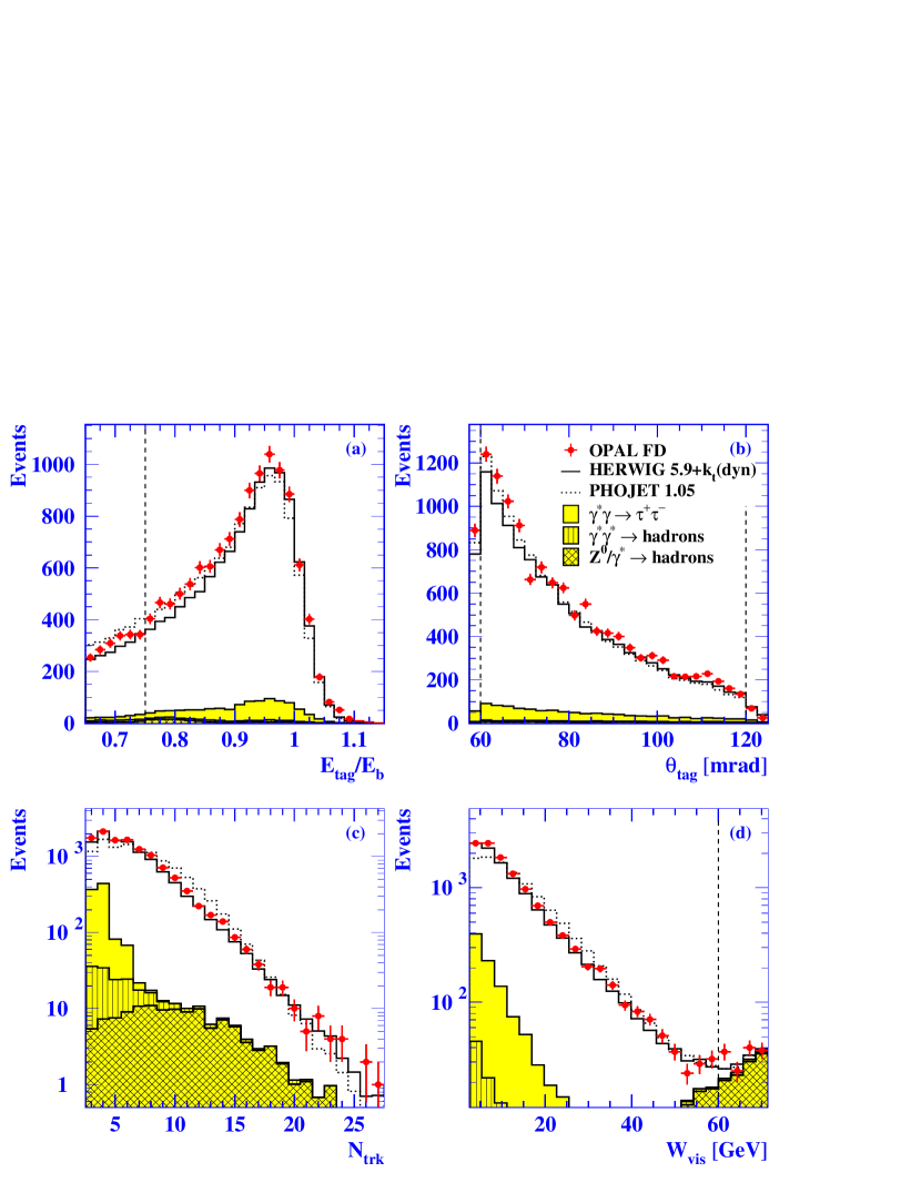
Figure 1: Comparison of data distributions for the FD sample with Monte Carlo predictions. The open histograms are the sum of the signal prediction and the contributions of the major background sources, shown both for the HERWIG (full lines) and PHOJET (dotted lines) models. The Monte Carlo predictions are normalised to the data luminosity, except for PHOJET where the sample has been normalised such that the predicted number of events for the SW sample is the same as that of HERWIG. All selection cuts have been applied, except for any cut on the variable in the plot (indicated as dashed lines if within the region shown). The distributions are: (a) $E_{\mathrm{tag}}$/$E_{\mathrm{b}}$, the energy of the scattered electron as a fraction of the energy of the beam electrons; (b) $\theta_{\rm tag}$, the polar angle of the scattered electron; (c) $N_{\mathrm{trk}}$, the number of tracks originating from the hadronic final state; and (d) $W_{\mathrm{vis}}$, the measured invariant mass of the hadronic final state. The errors given are only statistical.

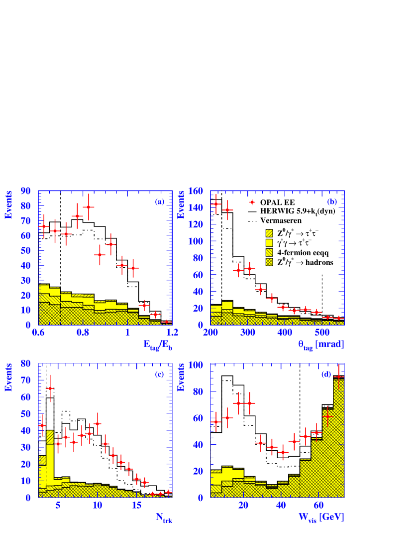
Figure 2: Comparison of data distributions for the EE sample with the Monte Carlo predictions. See Figure 1 for details.

Monte Carlo samples are used in an unfolding procedure to extract the differential cross-section ${\mathrm{d}}\sigma/{\mathrm{d}}x$ and $F_{2}^{\gamma}(x,Q^{2})$ from the data. Therefore, apart from explicit effects due to the variation of the structure function, a good description of the data distributions by the Monte Carlo is needed both for electron variables, which are used to measure $Q^{2}$, and for hadronic variables, which determine $W^{2}$. The analysis of the SW sample closely follows that presented in [19] but includes three times the data integrated luminosity. The quality of the description of this sample is similar to that presented in [19]. The analysis of the FD and EE samples at LEP2 energies is new. Figures 1 and 2 show comparisons between data and Monte Carlo distributions for these two samples. The quantities shown are (a) $E_{\mathrm{tag}}$/$E_{\mathrm{b}}$, the energy of the scattered electron as a fraction of the energy of the beam electrons, (b) $\theta_{\rm tag}$, the polar angle of the scattered electron, (c) $N_{\mathrm{trk}}$, the number of tracks originating from the hadronic final state, and (d) $W_{\mathrm{vis}}$, the measured invariant mass of the hadronic final state. The FD sample, Figure 1, is compared to the Monte Carlo prediction of the HERWIG and PHOJET (without reweighting of the $x$ distribution) signal events together with background estimates. The PHOJET sample has been normalised such that the predicted number of events for the SW sample is the same as that of HERWIG, so the PHOJET distributions only allow for a shape comparison. The HERWIG Monte Carlo model predicts slightly fewer events than are observed in the data and, in general, the shapes of the data distributions are better described by HERWIG than by PHOJET. The EE sample, Figure 2, is compared to the Monte Carlo prediction of the HERWIG and Vermaseren signal events together with background estimates. The data distributions of the energy and polar angle of the scattered electron are well described by the Monte Carlo predictions. For the variables related to the hadronic final state there are apparent differences in shape.

The hadronic energy flow for the SW sample has been studied in [19]. On average, about 5$\%$ of the energy is deposited in SW, and about 20-25$\%$ in FD and SW combined. The numbers for the FD and EE sample are even lower. It was verified that scaling the energy in the forward region has a small impact on the measured $F_{2}^{\gamma}$ for $x>0.1$. Consequently, in the present analysis this energy is not scaled.

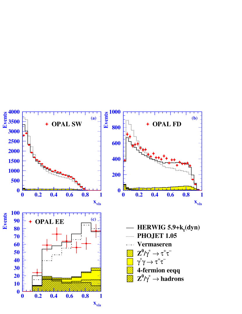
Figure 3: The measured $x_{\mathrm{vis}}$ distributions for the three samples (a) SW, (b) FD and (c) EE. The data are compared to Monte Carlo predictions containing signal and background contributions normalised to the data luminosity, except for PHOJET where the sample has been normalised such that the predicted number of events for the SW sample is the same as that of HERWIG. The errors given are only statistical.

The quantity $x_{\mathrm{vis}}$, obtained from $Q^{2}$ and $W_{\mathrm{vis}}$, is shown in Figure 3 for the three samples. It should be noted that for the SW sample, for $x_{\mathrm{vis}}>0.1$, the HERWIG model using the GRV parameterisation of $F_{2}^{\gamma}$ qualitatively follows the data, which means that the $F_{2}^{\gamma}$ found from the data should be similar to the expectation from GRV. In contrast, for the FD sample for $0.1<x_{\mathrm{vis}}<0.7$ the HERWIG prediction is systematically lower than the data. Due to the shortcoming of the PHOJET model discussed above, the description of the $x_{\mathrm{vis}}$ distribution is unsatisfactory when using the PHOJET model without reweighting of the $x$ distribution. For the EE sample the difference in shape of the $W_{\mathrm{vis}}$ distribution is reflected in the observed difference between the data and both Monte Carlo models for the $x_{\mathrm{vis}}$ distribution.

5.2 Measurement of ${\mathrm{d}}\sigma/{\mathrm{d}}x$ and $F_{2}^{\gamma}$ at high $Q^{2}$

The differential cross-section ${\mathrm{d}}\sigma/{\mathrm{d}}x$ and the structure function $F_{2}^{\gamma}$ are obtained from the data by unfolding the $x_{\mathrm{vis}}$ distribution of the EE sample, after applying additional cuts on $Q^{2}$. The main problem in measurements of $F_{2}^{\gamma}$ at low $x$, i.e. $x<0.1$, is the dependence of $F_{2}^{\gamma}$ on the Monte Carlo modelling, which enters when the unfolding process is used to relate the visible distributions to the underlying $x$ distribution. This problem is less severe at medium to large values of $x$, in particular for the high $Q^{2}$ EE sample, where the hadronic final state has much more transverse momentum and as a consequence is better contained in the detector. Therefore the correlation between the measured invariant mass $W_{\mathrm{vis}}$ and the true $W$, e.g. as given by HERWIG, is much better at large $x$, so the results can be expected to have a smaller dependence on the Monte Carlo modelling of the hadronic final state.

No attempt has been made in this analysis to access the region of $x<0.1$, so using a one dimensional unfolding on a linear scale in $x$ is appropriate, in contrast with [19]. For this purpose the RUN program [23] has been used. Technically, RUN uses a set of Monte Carlo events which are based on an input $F_{2}^{\gamma}(x,Q^{2})$ and carry the information about the correlation of $x_{\mathrm{vis}}$ and $x$. A continuous weight function is defined which depends only on $x$. This function is constructed from individual weight factors for each Monte Carlo event. These weight factors are obtained by fitting the $x_{\mathrm{vis}}$ distribution of the Monte Carlo sample to the measured $x_{\mathrm{vis}}$ distribution of the data, such that the reweighted Monte Carlo events describe the $x_{\mathrm{vis}}$ distribution of the data as well as possible. After the unfolding the two $x_{\mathrm{vis}}$ distributions are consistent. The unfolded $F_{2}^{\gamma}(x,Q^{2})$ from the data is then obtained by multiplying the input $F_{2}^{\gamma}(x,Q^{2})$ of the Monte Carlo with the weight function. For further details the reader is referred to [1]. It has been demonstrated in [19] that this procedure is independent of the input structure function used in the Monte Carlo.

Radiative corrections and the dependence of $F_{2}^{\gamma}(x,Q^{2},P^{2})$ on $P^{2}$ are treated as in the previous OPAL analysis [19]. The radiative corrections applied to the data have been estimated using the RADEG program [24]. They are obtained for each bin in $x$ and $Q^{2}$ using the SaS1D [25] prediction of $F_{2}^{\gamma}$. No correction for the effect of non-zero $P^{2}$ has been made, see Refs. [19, 1] for further details. The average value of $P^{2}$ of the data samples as predicted by the HERWIG program is about 0.2 $\mathrm{GeV}^{2}$. Note however that HERWIG does not take into account the $P^{2}$ dependence of $F_{2}^{\gamma}$.

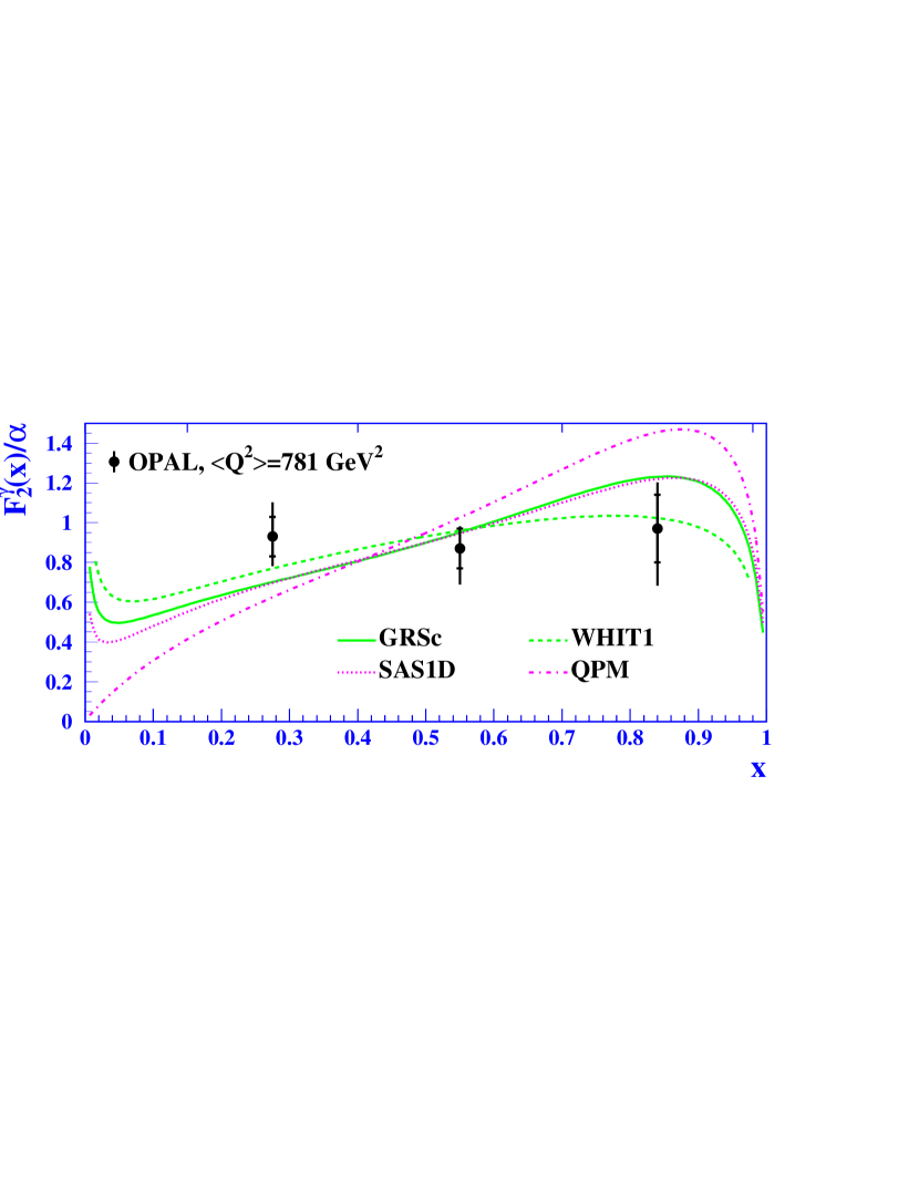
Figure 4: The measured $F_{2}^{\gamma}/\alpha$ as a function of $x$ for the EE sample. The data are unfolded for $\langle Q^{2}\rangle=780$ $\mathrm{GeV}^{2}$ and compared to the leading order predictions from the GRSc (full line), SaS1D (dotted line), WHIT1 (dashed line) and QPM (dot-dashed line) parameterisations of $F_{2}^{\gamma}/\alpha$. The inner error bars represent the statistical errors and the outer error bars represent statistical and systematic errors added in quadrature. The tick marks at the top of the figure represent the bin boundaries.

After subtraction of background, the EE sample has been unfolded using three bins in $x$ spanning the range $0.15-0.98$ and for $400<Q^{2}<2350$ $\mathrm{GeV}^{2}$. The central values are obtained using HERWIG as the input Monte Carlo model for the unfolding. Each data point is corrected for radiative effects as described above. Bin-centre corrections are also applied as given by the average of the GRSc [26], SaS1D and WHIT1 [27] predictions for the correction from the average $F_{2}^{\gamma}$ over the bin to the value of $F_{2}^{\gamma}$ at the nominal $x$ position. The result for $F_{2}^{\gamma}/\alpha$ is shown in Figure 4 and listed in Table 3 together with the correlation matrix. In each bin of $x$ the result for ${\mathrm{d}}\sigma/{\mathrm{d}}x$ is also listed. The ${\mathrm{d}}\sigma/{\mathrm{d}}x$ values are corrected to the phase space given by the $Q^{2}$ range and $y<0.3$.

Systematic errors are estimated by repeating the unfolding with one parameter varied at a time and determining the shift in the result. The systematic errors are combined by adding all individual contributions in quadrature separately for positive and negative contributions. The systematic effects considered for the EE sample are:

• Model dependence:
  The dependence on the Monte Carlo model used in the unfolding has been estimated by repeating the unfolding using the Vermaseren sample and taking the full difference as the systematic error, both for the positive and negative error.

• Variations of cuts:
  The composition of the selected events was varied by changing the cuts one at a time. The size of the variations reflect the resolution of the measured variables and the description of the data by the Monte Carlo models around the cut values. The variations are sufficiently small not to change the average $Q^{2}$ of the sample significantly. The variations made are listed in Table 1.

• Unfolding parameters:
  The number of bins used for the measured variable can be different from the number used for the true variable. The standard result has 5 bins in the measured variable. This was in turn reduced to 4 and increased to 6 to estimate the systematic effects of the unfolding.

• Calibration of the tagging detector:
  The energy of the scattered electron in the Monte Carlo samples was conservatively scaled by $\pm 1\%$ [28].

• Measurement of the hadronic energy:
  The main uncertainty is in the calibration of the response of the electromagnetic calorimeter to hadronic energy for low energy particles in the hadronic final state. The absolute energy scale was varied by $\pm 3\%$ [29] in the Monte Carlo samples.

• Background modelling:
  To quantify the uncertainty on the most dominant background, stemming from the reaction $\mathrm{Z}^{0}/\gamma^{\star}\to\mbox{hadrons}$, the KK program along with cluster fragmentation from HERWIG has been used instead of PYTHIA with string fragmentation.

• Cone size for the $W_{\mathrm{vis}}$ calculation:
  The size of the exclusion cone for the $W_{\mathrm{vis}}$ calculation of 200 mrad half-angle about the direction of the scattered electron has been varied by $\pm 30$ mrad.

The size of the contributions to the error from the individual sources is similar and no single source is dominant. When combining all error sources, the total estimated systematic error is of the same order as the statistical error.

The measured $F_{2}^{\gamma}/\alpha$, shown in Figure 4 together with several theoretical calculations, exhibits a flat behaviour. The leading order parameterisations of $F_{2}^{\gamma}$ from GRSc, SaS1D and WHIT1, which all include a contribution from massive charm quarks, are described in detail in [1]. The contribution from bottom quarks is negligible. It can be seen that in this high $Q^{2}$ regime the differences between these predictions are moderate, particularly in the central $x$-region. All these predictions are compatible with the data to within about 20$\%$, with the WHIT1 parameterisation, which predicts the flattest behaviour, being closest to the data. The QPM curve, which models only the point-like component of $F_{2}^{\gamma}$, is calculated for four active flavours with masses of 0.325 $\mathrm{GeV}$ for light quarks and 1.5 $\mathrm{GeV}$ for charm quarks. This prediction shows a much steeper behaviour in $x$ and is disfavoured by the data.

5.3 Measurement of the $Q^{2}$ evolution of $F_{2}^{\gamma}$

Following the study of the scaling violation of $F_{2}^{\gamma}$ performed in [30] the evolution of $F_{2}^{\gamma}$ with $Q^{2}$ has been measured for several $x$ ranges using all three samples. Due to their large statistics, the SW and FD samples are further split into two bins of $Q^{2}$ (9–15 and 15–30 $\mathrm{GeV}^{2}$ for SW and 30–50 and 50–150 $\mathrm{GeV}^{2}$ for FD). The data are unfolded as a function of $x$ separately in each bin of $Q^{2}$ and corrected for radiative effects. The results are shown in Figure 5 and listed in Table 4. The estimation of the systematic errors for the EE sample is described above. For the SW and FD samples the estimation of the systematic error mirrors the procedure for the EE sample, with some differences. The PHOJET program is used as a second Monte Carlo to determine the model dependence; the variations of cuts are given in Table 1. For the unfolding parameters the standard number of bins, which was 8 for the central values, has been varied by $\pm 2$. No systematics due to the electron isolation are needed for the SW and FD samples. For these samples, the largest contribution to the systematic error generally stems from the estimated model dependence. With only two models available that satisfactorily describe the data [19], the estimated systematic error is small for those $x,Q^{2}$ regions where the two models happen to predict similar correlations between $x$ and $x_{\mathrm{vis}}$. To reduce fluctuations within the SW and FD samples, the systematic error from this source has been averaged for each region of $x$ for the two $Q^{2}$ points within a given sample.

The data in Figure 5(a) show positive scaling violations in $F_{2}^{\gamma}$ for the $x$ ranges 0.10–0.25 and 0.25–0.60. The QCD inspired parametrisations of $F_{2}^{\gamma}$ qualitatively follow the data, but do not perfectly account for them. For the SW sample the GRSc and SaS1D predictions, which are almost indistinguishable, closely resemble the data, whereas at higher $Q^{2}$, for the FD sample, WHIT1 comes closest. For the range 0.60–0.85, the data are compatible with the predicted scaling violations of the QCD inspired parametrisations. The QPM model generally gives a bad description of the data, especially at low $x$.

To quantify the slope for medium values of $x$, where data are available at all values of $Q^{2}$, the data are fitted using essentially the procedure from [30]. A linear function of the form $a+b\,\ln\,Q^{2}$, where $Q^{2}$ is in $\mathrm{GeV}^{2}$, has been fitted to the data in the region 0.10–0.60. Within this range of $x$ the parameters $a$ and $b$ are assumed to be independent of $x$. To obtain the central values of the two parameters, with their statistical errors and correlation, a fit was performed by the MINUIT [31] program using the measured values of $F_{2}^{\gamma}/\alpha$ and their statistical errors as listed in Table 4. The fit was repeated for each of the systematic variations. The systematic errors of $a$ and $b$ are estimated as the quadratic sum of the deviations of the two parameters from the central values. The result of the fit is

$$F_{2}^{\gamma}(Q^{2})/\alpha=(0.08\,\pm 0.02\,^{+\,0.05}_{-\,0.03})+(0.13\,\pm 0.01\,^{+\,0.01}_{-\,0.01})\,\ln\,Q^{2}\,,$$

with, for the central result, a correlation between the two parameters of $-0.98$ and a $\chi^{2}$ of 10 for 3 degrees of freedom. No significant change of the result is observed if the fit is performed using the full error on each point. This new result compares to the previous OPAL value [30] of

$$F_{2}^{\gamma}(Q^{2})/\alpha=(0.16\,\pm 0.05\,^{+\,0.17}_{-\,0.16})+(0.10\,\pm 0.02\,^{+\,0.05}_{-\,0.02})\,\ln\,Q^{2}.$$

These two determinations, based on independent data sets, are in agreement, and the errors on $a$ and $b$ have been significantly reduced. The data, together with the fit result, are shown in Figure 5(b). They are qualitatively described by the higher order GRV parametrisation (GRV HO).

6 Conclusions

The photon structure function $F_{2}^{\gamma}$ and the differential cross-section ${\mathrm{d}}\sigma/{\mathrm{d}}x$ have been measured using deep inelastic electron-photon scattering events recorded by the OPAL detector during the years 1997–2000 with an integrated luminosity of 632 $\mathrm{pb}^{-1}$ and an average $\mathrm{e}^{+}\mathrm{e}^{-}$ centre-of-mass energy of 197.1 GeV.

The structure function $F_{2}^{\gamma}$ has been measured as a function of $x$ in the range $0.15<x<0.98$ and at an average photon virtuality of $\langle Q^{2}\rangle=780$ $\mathrm{GeV}^{2}$, which represents the highest value measured so far. The $Q^{2}$ evolution of $F_{2}^{\gamma}$ has been studied for $12.1<\langle Q^{2}\rangle<780$ $\mathrm{GeV}^{2}$ using several ranges of $x$. The data exhibit positive scaling violations in $F_{2}^{\gamma}$ for the $x$ ranges 0.10–0.25 and 0.25–0.60. For the range 0.60–0.85, the data are compatible with the predicted scaling violations. The measured evolution of $F_{2}^{\gamma}/\alpha$ as a function of $Q^{2}$ in the central region of $x$, 0.10–0.60, has been fitted with a linear function in $\ln Q^{2}$, resulting in

$$F_{2}^{\gamma}(Q^{2})/\alpha=(0.08\,\pm 0.02\,^{+\,0.05}_{-\,0.03})+(0.13\,\pm 0.01\,^{+\,0.01}_{-\,0.01})\,\ln\,Q^{2}\,,$$

where $Q^{2}$ is in $\mathrm{GeV}^{2}$.

Both for the measurement of $F_{2}^{\gamma}$ at $\langle Q^{2}\rangle=780$ $\mathrm{GeV}^{2}$ and for the investigation of the $Q^{2}$ evolution of $F_{2}^{\gamma}$, the quark-parton model prediction is not in agreement with the data. It shows a much steeper rise than the data as a function of $x$ for $\langle Q^{2}\rangle=780$ $\mathrm{GeV}^{2}$ and also a different behaviour in the $Q^{2}$ evolution. In contrast, the leading order GRSc, SaS1D and WHIT1 parameterisations and the higher order GRV parameterisation of $F_{2}^{\gamma}$ are much closer to the data. This means that the corresponding parton distribution functions of the photon are adequate to within about 20$\%$ at large values of $x$ and at $\langle Q^{2}\rangle$ scales of about 780 $\mathrm{GeV}^{2}$.

Acknowledgements:

We particularly wish to thank the SL Division for the efficient operation of the LEP accelerator at all energies and for their close cooperation with our experimental group. We thank our colleagues from CEA, DAPNIA/SPP, CE-Saclay for their efforts over the years on the time-of-flight and trigger systems which we continue to use. In addition to the support staff at our own institutions we are pleased to acknowledge the
Department of Energy, USA,
National Science Foundation, USA,
Particle Physics and Astronomy Research Council, UK,
Natural Sciences and Engineering Research Council, Canada,
Israel Science Foundation, administered by the Israel Academy of Science and Humanities,
Minerva Gesellschaft,
Benoziyo Center for High Energy Physics,
Japanese Ministry of Education, Science and Culture (the Monbusho) and a grant under the Monbusho International Science Research Program,
Japanese Society for the Promotion of Science (JSPS),
German Israeli Bi-national Science Foundation (GIF),
Bundesministerium für Bildung und Forschung, Germany,
National Research Council of Canada,
Research Corporation, USA,
Hungarian Foundation for Scientific Research, OTKA T-029328, T023793 and OTKA F-023259,
Fund for Scientific Research, Flanders, F.W.O.-Vlaanderen, Belgium.

Cut $\backslash$ Sample	SW	FD	EE
$E_{\mathrm{tag}}$/$E_{\mathrm{b}}$ min	$0.75\,(\pm 0.05)$		$0.70\,(\pm 0.05)$
$\theta_{\rm tag}$ min [mrad]	$33.25\,(+2)$	$60\,(+3)$	$230\,(\pm 5)$
$\theta_{\rm tag}$ max [mrad]	$55\,(-2)$	$120\,(-3)$	$500\,(\pm 5)$
$E_{\mathrm{a}}$/$E_{\mathrm{b}}$ max	$0.25\,(\pm 0.05)$
$N_{\mathrm{trk}}$ min	$3\,(+1)$		$4\,(+1)$
	(2 non-electron tracks)
$W_{\mathrm{vis}}$ min $[\mathrm{GeV}]$	$2.5\,(+1)$
$W_{\mathrm{vis}}$ max $[\mathrm{GeV}]$	$60\,(\pm 5)$		$50\,(\pm 5)$
Electron isolation $[\mathrm{GeV}]$	-		$3.0\,(\pm 0.5)$

Table 1: The selection cuts applied to each data sample, together with the variations applied (in brackets). See the text for explanation of the variables.

		SW		FD		EE
data selected		27819		11874		414
data signal		26071$\,\pm\,$	167	10652$\,\pm\,$	110	274$\,\pm\,$	21
Monte Carlo selected		28308$\,\pm\,$	51	11211$\,\pm\,$	32	436$\,\pm\,$	6
HERWIG signal		26560$\,\pm\,$	49	9989$\,\pm\,$	30	296$\,\pm\,$	5
	$\gamma^{\star}\gamma\to\tau^{+}\tau^{-}$	1309.3$\,\pm\,$	14.1	845.5$\,\pm\,$	11.3	31.8$\,\pm\,$	2.2
	$\gamma^{\star}\gamma^{\star}\rightarrow\mbox{hadrons}$	321.3$\,\pm\,$	4.7	193.4$\,\pm\,$	3.7	5.0$\,\pm\,$	0.3
	$\mathrm{Z}^{0}/\gamma^{\star}\to\mbox{hadrons}$	82.8$\,\pm\,$	2.4	124.6$\,\pm\,$	3.1	76.2$\,\pm\,$	2.4
	$\mathrm{Z}^{0}/\gamma^{\star}\rightarrow\tau^{+}\tau^{-}$	7.9$\,\pm\,$	0.3	10.5$\,\pm\,$	0.4	10.6$\,\pm\,$	0.4
Backgrounds	4-fermion eeqq	27.0$\,\pm\,$	0.9	48.2$\,\pm\,$	1.1	16.6$\,\pm\,$	0.7

Table 2: The numbers of selected events and signal events (selected events corrected for background) in the data compared to the signal predictions from the HERWIG program. The expected numbers of background events for the dominant sources according to Monte Carlo are also listed. The errors given are only statistical.

$x$	$x$	$F_{2}^{\gamma}/\alpha$	${\mathrm{d}}\sigma/{\mathrm{d}}x$	radiative	bin-centre
range	bin-centre		[pb]	cor. [$\%$]	cor. [$\%$]
$0.15-0.40$	$0.275$	$0.93\,\pm 0.10\,^{+\,0.14}_{-\,0.11}$	$0.94\,\pm 0.11\,^{+\,0.15}_{-\,0.11}$	$-8.8$	$-0.4$
$0.40-0.70$	$0.550$	$0.87\,\pm 0.10\,^{+\,0.05}_{-\,0.15}$	$0.79\,\pm 0.09\,^{+\,0.05}_{-\,0.14}$	$-6.9$	$\phantom{-}0.1$
$0.70-0.98$	$0.840$	$0.97\,\pm 0.17\,^{+\,0.16}_{-\,0.23}$	$0.62\,\pm 0.11\,^{+\,0.10}_{-\,0.15}$	$-5.4$	$-5.1$

$x$ range	$0.15-0.40$	$0.40-0.70$	$0.70-0.98$
$0.15-0.40$	$\phantom{-}1.00$
$0.40-0.70$	$\phantom{-}0.16$	$\phantom{-}1.00$
$0.70-0.98$	$-0.04$	$-0.15$	$1.00$

Table 3: Results for the EE sample for $F_{2}^{\gamma}/\alpha$ as a function of $x$ at $\langle Q^{2}\rangle$ of 780 $\mathrm{GeV}^{2}$, and for ${\mathrm{d}}\sigma/{\mathrm{d}}x$ in the $Q^{2}$ range 400-2350 $\mathrm{GeV}^{2}$ and $y<0.3$. The first errors are statistical and the second systematic. The data were unfolded in bins defined by the $x$ ranges and corrected for radiative effects. For a given bin the radiative correction is the difference of the radiative and non-radiative cross-sections as a percentage of the non-radiative cross-section. The structure function was corrected to the $x$ values listed using the bin-centre corrections which are given as a percentage of the non-corrected $F_{2}^{\gamma}$. The statistical correlations between the bins for the central result are also given.

(a)
$x$ range	$Q^{2}$ range	$\langle Q^{2}\rangle$	$F_{2}^{\gamma}/\alpha$	${\mathrm{d}}\sigma/{\mathrm{d}}x$			radiative
	$[\mathrm{GeV}^{2}]$	$[\mathrm{GeV}^{2}]$		[pb]			cor. [$\%$]
$0.10-0.25$	$\phantom{0}\phantom{0}9-15\phantom{0}\phantom{0}$	12.1	$0.38\,\pm 0.01\,^{+\,0.03}_{-\,0.03}$	83 $\,\pm\,$	1 $\,{}^{+\,}_{-\,}$	${}^{7}_{6}$	$-5.3$
$0.25-0.60$			$0.43\,\pm 0.01\,^{+\,0.03}_{-\,0.02}$	47 $\,\pm\,$	1 $\,{}^{+\,}_{-\,}$	${}^{4}_{2}$	$-4.4$
$0.10-0.25$	$\phantom{0}15-30\phantom{0}\phantom{0}$	19.9	$0.39\,\pm 0.01\,^{+\,0.03}_{-\,0.03}$	56 $\,\pm\,$	1 $\,{}^{+\,}_{-\,}$	${}^{4}_{4}$	$-5.5$
$0.25-0.60$			$0.49\,\pm 0.01\,^{+\,0.02}_{-\,0.02}$	36 $\,\pm\,$	1 $\,{}^{+\,}_{-\,}$	${}^{1}_{1}$	$-4.5$
$0.10-0.25$	$\phantom{0}30-50\phantom{0}\phantom{0}$	39.7	$0.47\,\pm 0.01\,^{+\,0.02}_{-\,0.02}$	21.7 $\,\pm\,$	0.4 $\,{}^{+\,}_{-\,}$	${}^{0.9}_{0.9}$	$-5.9$
$0.25-0.60$			$0.63\,\pm 0.01\,^{+\,0.02}_{-\,0.03}$	15.9 $\,\pm\,$	0.4 $\,{}^{+\,}_{-\,}$	${}^{0.5}_{0.7}$	$-4.8$
$0.60-0.85$			$0.65\,\pm 0.03\,^{+\,0.06}_{-\,0.06}$	$\phantom{1}9.6$ $\,\pm\,$	0.4 $\,{}^{+\,}_{-\,}$	${}^{0.9}_{0.8}$	$-3.8$
$0.10-0.25$	$\phantom{0}50-150\phantom{0}$	76.4	$0.55\,\pm 0.01\,^{+\,0.02}_{-\,0.03}$	18.8 $\,\pm\,$	0.4 $\,{}^{+\,}_{-\,}$	${}^{0.7}_{0.9}$	$-6.5$
$0.25-0.60$			$0.68\,\pm 0.01\,^{+\,0.02}_{-\,0.02}$	13.8 $\,\pm\,$	0.3 $\,{}^{+\,}_{-\,}$	${}^{0.4}_{0.4}$	$-5.2$
$0.60-0.85$			$0.73\,\pm 0.02\,^{+\,0.04}_{-\,0.04}$	$\phantom{1}9.1$ $\,\pm\,$	0.3 $\,{}^{+\,}_{-\,}$	${}^{0.4}_{0.5}$	$-4.1$
$0.25-0.60$	$400-2350$	780	$0.94\,\pm 0.09\,^{+\,0.09}_{-\,0.11}$	0.91 $\,\pm\,$	0.09 $\,{}^{+\,}_{-\,}$	${}^{0.08}_{0.10}$	$-7.6$
$0.60-0.85$			$0.83\,\pm 0.11\,^{+\,0.21}_{-\,0.29}$	0.71 $\,\pm\,$	0.09 $\,{}^{+\,}_{-\,}$	${}^{0.18}_{0.25}$	$-6.0$

$x$ range	$0.10-0.25$	$0.25-0.60$	$0.60-0.85$
$0.10-0.25$	1
$0.25-0.60$	0.00/0.28/0.45/0.40/–	1
$0.60-0.85$	–/–/-0.23/-0.19/–	–/–/0.32/0.27/0.17	1

(b)
$x$ range	$Q^{2}$ range	$\langle Q^{2}\rangle$	$F_{2}^{\gamma}/\alpha$	${\mathrm{d}}\sigma/{\mathrm{d}}x$			radiative
	$[\mathrm{GeV}^{2}]$	$[\mathrm{GeV}^{2}]$		[pb]			cor. [$\%$]
$0.10-0.60$	$\phantom{0}\phantom{0}9-15\phantom{0}\phantom{0}$	12.1	$0.41\,\pm 0.01\,^{+\,0.03}_{-\,0.02}$	57 $\,\pm\,$	1 $\,{}^{+\,}_{-\,}$	${}^{4}_{2}$	$-4.7$
	$\phantom{0}15-30\phantom{0}\phantom{0}$	19.9	$0.46\,\pm 0.01\,^{+\,0.01}_{-\,0.01}$	42 $\,\pm\,$	1 $\,{}^{+\,}_{-\,}$	${}^{1}_{1}$	$-4.9$
	$\phantom{0}30-50\phantom{0}\phantom{0}$	39.7	$0.58\,\pm 0.01\,^{+\,0.02}_{-\,0.02}$	17.7 $\,\pm\,$	0.3 $\,{}^{+\,}_{-\,}$	${}^{0.6}_{0.7}$	$-5.3$
	$\phantom{0}50-150\phantom{0}$	76.4	$0.64\,\pm 0.01\,^{+\,0.02}_{-\,0.02}$	15.3 $\,\pm\,$	0.3 $\,{}^{+\,}_{-\,}$	${}^{0.4}_{0.5}$	$-5.6$
	$400-2350$	780	$0.90\,\pm 0.09\,^{+\,0.13}_{-\,0.11}$	0.86 $\,\pm\,$	0.08 $\,{}^{+\,}_{-\,}$	${}^{0.12}_{0.11}$	$-8.2$

Table 4: Results for the average $F_{2}^{\gamma}/\alpha$ in bins of $x$ for several values of $\langle Q^{2}\rangle$ and for ${\mathrm{d}}\sigma/{\mathrm{d}}x$ for several ranges of $Q^{2}$. Section (a) corresponds to Figure 5(a), section (b) to Figure 5(b) The first errors are statistical and the second systematic. The data were unfolded in bins defined by the $x$ and $Q^{2}$ ranges listed. The radiative corrections which have been applied are also listed. For a given bin the radiative correction is the difference of the radiative and non-radiative cross-sections as a percentage of the non-radiative cross-section. The statistical correlations between the bins for the central result for the $\langle Q^{2}\rangle$ values 12.1/19.9/39.7/76.4/780 $\mathrm{GeV}^{2}$ are also given.

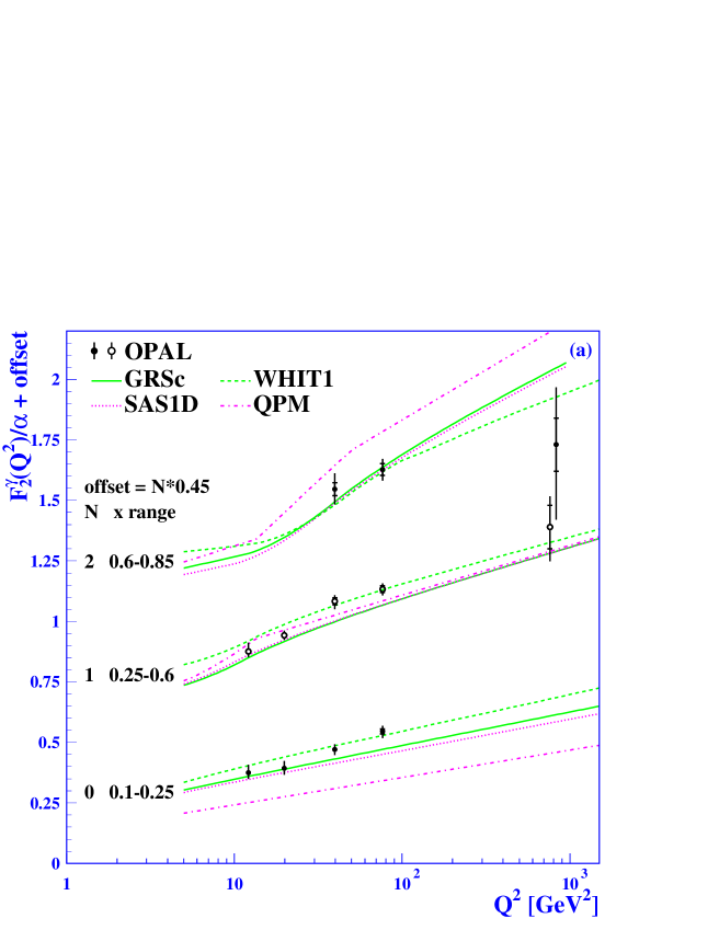
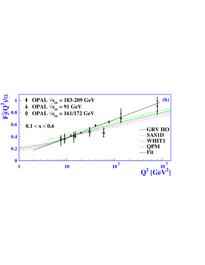
Figure 5: The evolution of $F_{2}^{\gamma}/\alpha$ as a function of $Q^{2}$ for several bins of $x$, (a) 0.10–0.25, 0.25–0.60 and 0.60–0.85 and (b) for the central region 0.10–0.60. The inner error bars represent the statistical errors and the outer error bars represent statistical and systematic errors added in quadrature. In (a) the data are compared to the predictions from the GRSc (full line), SaS1D (dotted line), WHIT1 (dashed line), and QPM (dot-dashed line) parameterisations of $F_{2}^{\gamma}/\alpha$. In (b) GRSc has been replaced by the higher order prediction from GRV and, in addition, the result of the fit is shown.

References

- [1] R. Nisius, Phys. Rep. 332, 165–317 (2000).
-
[2]
V.N. Gribov and L.N. Lipatov,
Sov. J. Nucl. Phys. 15, 438–450 (1972);
L.N. Lipatov, Sov. J. Nucl. Phys. 20, 94–102 (1975);
G. Altarelli and G. Parisi, Nucl. Phys. B126, 298–318 (1977);
Y.L. Dokshitzer, Sov. Phys. JETP 46, 641–653, (1977). -
[3]
C.F. von Weizsäcker, Z. Phys. 88, 612–625 (1934);
E.J. Williams, Phys. Rev. 45, 729–730 (1934);
V.M. Budnev, I.F. Ginzburg, G.V. Meledin, and V.G. Serbo, Phys. Rep. 15, 181–282 (1975). - [4] ZEUS Collaboration, J. Breitweg et al., Eur. Phys. J. C11, 35–50 (1999).
- [5] K. Long, R. Nisius, and W.J. Stirling, Summary of the structure function session at DIS01, in 9th International Workshop on Deep Inelastic Scattering and QCD, DIS2001 Conference, Bologna, Italy, 27 April - 1 May 2001, World Scientific, 2001, hep-ph/0109092, and references therein.
- [6] OPAL Collaboration, K. Ahmet et al., Nucl. Instr. and Meth. A305, 275–319 (1991).
-
[7]
P.P. Allport et al., Nucl. Instr. and Meth. A324, 34–52 (1993);
P.P. Allport et al., Nucl. Instr. and Meth. A346, 476–495 (1994). - [8] B.E. Anderson et al., IEEE Transactions on Nuclear Science 41, 845–852 (1994).
- [9] OPAL Collaboration, G. Abbiendi et al., Measurement of the hadronic cross-section for the scattering of two virtual photons at LEP, CERN-EP-2001-064, submitted to Eur. Phys. J.C.
- [10] OPAL Collaboration, G. Alexander et al., Phys. Lett. B377, 181–194 (1996).
- [11] J. Allison et al., Nucl. Instr. and Meth. A317, 47–74 (1992).
- [12] G. Marchesini et al., Comp. Phys. Comm. 67, 465–508 (1992).
-
[13]
R. Engel, Z. Phys. C66, 203–214 (1995);
R. Engel and J. Ranft, Phys. Rev. D54, 4244–4262 (1996). -
[14]
J.A.M. Vermaseren, J. Smith, and G. Grammer Jr.,
Phys. Rev. D19, 137–143 (1979);
J.A.M. Vermaseren, Nucl. Phys. B229, 347–371 (1983). - [15] The LEP Working Group for Two-Photon Physics, ALEPH, L3, and OPAL, Comparison of Deep Inelastic Electron-Photon Scattering Data with the Herwig and Phojet Monte Carlo Models, CERN-EP-2000-109, hep-ex/0010041, submitted to Eur. Phys. J.C.
- [16] T. Sjöstrand et al., Comp. Phys. Comm. 135, 238–259 (2001).
-
[17]
M. Glück, E. Reya, and A. Vogt, Phys. Rev. D45, 3986–3994 (1992);
M. Glück, E. Reya, and A. Vogt, Phys. Rev. D46, 1973–1979 (1992). - [18] H. Plothow-Besch, Comp. Phys. Comm. 75, 396–416 (1993).
- [19] OPAL Collaboration, G. Abbiendi et al., Eur. Phys. J. C18, 15–39 (2000).
-
[20]
T. Sjöstrand, CERN-TH/93-7112 (1993);
T. Sjöstrand, Comp. Phys. Comm. 82, 74–89 (1994). - [21] J. Fujimoto et al., Comp. Phys. Comm. 100, 128–156 (1997).
- [22] S. Jadach, B.F.L. Ward, and Z. Wa̧s, Comp. Phys. Comm. 130, 260–325 (2000).
-
[23]
V. Blobel, Unfolding methods in high-energy physics experiments,
DESY/84-118 (1984);
V. Blobel, Regularized Unfolding for High-Energy Physics Experiments, RUN program manual, unpublished (1996). -
[24]
E. Laenen and G.A. Schuler, Phys. Lett. B374, 217–224 (1996);
E. Laenen and G.A. Schuler, Model-independent QED corrections to photon structure-function measurements, in PHOTON97, Incorporating the XIth International Workshop on GammaGamma Collisions, Egmond aan Zee, 10-15 May, 1997, edited by A. Buijs and F.C. Erné, pages 57–62, World Scientific, 1998. - [25] G.A. Schuler and T. Sjöstrand, Z. Phys. C68, 607–624 (1995).
- [26] M. Glück, E. Reya, and I. Schienbein, Phys. Rev. D60, 054019 (1999).
- [27] K. Hagiwara, T. Izubuchi, M. Tanaka, and I. Watanabe, Phys. Rev. D51, 3197–3219 (1995).
- [28] OPAL Collaboration, G. Abbiendi et al., Eur. Phys. J. C13, 553–572 (2000).
- [29] OPAL Collaboration, G. Abbiendi et al., Eur. Phys. J. C14, 199–212 (2000).
- [30] OPAL Collaboration, K. Ackerstaff et al., Phys. Lett. B411, 387–401 (1997).
- [31] F. James and M. Ross, MINUIT-function minimization and error analysis, version 95.03, CERN Program Library D506, CERN (1995).