Measurement of the Ratio of Branching Fractions
of the $\Upsilon$(4S) to Charged and Neutral $B$ Mesons

Abstract

The ratio of charged and neutral $B$ meson production at the $\Upsilon$(4S), $f_{+-}/f_{00}$, is measured through the decays $\bar{B}\rightarrow D^{*}\ell^{-}\bar{\nu}_{\ell}$, reconstructed using a partial reconstruction method where the $D^{*}$ is detected only through a pion daughter from the decay $D^{*}\rightarrow D\pi$. Using data collected by the CLEO II detector, the charged and neutral $B$ decays are measured in such a way that their ratio is independent of decay model, limited mainly by the uncertainty in the relative efficiency for detecting neutral and charged pions. This measurement yields the ratio of production fractions times the ratio of semileptonic branching fractions, $f_{+-}b_{+}\over f_{00}b_{0}$. Assuming that $b_{+}\over b_{0}$ is equal to the lifetime ratio $\tau_{+}\over\tau_{0}$ and using the world average value of $\tau_{+}\over\tau_{0}$ as input, we obtain $f_{+-}/f_{00}=1.058\pm 0.084\pm 0.136$.

S. B. Athar,¹ P. Avery,¹ H. Stoeck,¹ J. Yelton,¹ G. Brandenburg,² A. Ershov,² D. Y.-J. Kim,² R. Wilson,² K. Benslama,³ B. I. Eisenstein,³ J. Ernst,³ G. D. Gollin,³ R. M. Hans,³ I. Karliner,³ N. Lowrey,³ M. A. Marsh,³ C. Plager,³ C. Sedlack,³ M. Selen,³ J. J. Thaler,³ J. Williams,³ K. W. Edwards,⁴ R. Ammar,⁵ D. Besson,⁵ X. Zhao,⁵ S. Anderson,⁶ V. V. Frolov,⁶ Y. Kubota,⁶ S. J. Lee,⁶ S. Z. Li,⁶ R. Poling,⁶ A. Smith,⁶ C. J. Stepaniak,⁶ J. Urheim,⁶ S. Ahmed,⁷ M. S. Alam,⁷ L. Jian,⁷ M. Saleem,⁷ F. Wappler,⁷ E. Eckhart,⁸ K. K. Gan,⁸ C. Gwon,⁸ T. Hart,⁸ K. Honscheid,⁸ D. Hufnagel,⁸ H. Kagan,⁸ R. Kass,⁸ T. K. Pedlar,⁸ J. B. Thayer,⁸ E. von Toerne,⁸ T. Wilksen,⁸ M. M. Zoeller,⁸ H. Muramatsu,⁹ S. J. Richichi,⁹ H. Severini,⁹ P. Skubic,⁹ S.A. Dytman,¹⁰ S. Nam,¹⁰ V. Savinov,¹⁰ S. Chen,¹¹ J. W. Hinson,¹¹ J. Lee,¹¹ D. H. Miller,¹¹ V. Pavlunin,¹¹ E. I. Shibata,¹¹ I. P. J. Shipsey,¹¹ D. Cronin-Hennessy,¹² A.L. Lyon,¹² C. S. Park,¹² W. Park,¹² E. H. Thorndike,¹² T. E. Coan,¹³ Y. S. Gao,¹³ F. Liu,¹³ Y. Maravin,¹³ I. Narsky,¹³ R. Stroynowski,¹³ J. Ye,¹³ M. Artuso,¹⁴ C. Boulahouache,¹⁴ K. Bukin,¹⁴ E. Dambasuren,¹⁴ R. Mountain,¹⁴ T. Skwarnicki,¹⁴ S. Stone,¹⁴ J.C. Wang,¹⁴ A. H. Mahmood,¹⁵ S. E. Csorna,¹⁶ I. Danko,¹⁶ Z. Xu,¹⁶ R. Godang,¹⁷ K. Kinoshita,^17, G. Bonvicini,¹⁸ D. Cinabro,¹⁸ M. Dubrovin,¹⁸ S. McGee,¹⁸ A. Bornheim,¹⁹ E. Lipeles,¹⁹ S. P. Pappas,¹⁹ A. Shapiro,¹⁹ W. M. Sun,¹⁹ A. J. Weinstein,¹⁹ G. Masek,²⁰ H. P. Paar,²⁰ R. Mahapatra,²¹ H. N. Nelson,²¹ R. A. Briere,²² G. P. Chen,²² T. Ferguson,²² G. Tatishvili,²² H. Vogel,²² N. E. Adam,²³ J. P. Alexander,²³ C. Bebek,²³ K. Berkelman,²³ F. Blanc,²³ V. Boisvert,²³ D. G. Cassel,²³ P. S. Drell,²³ J. E. Duboscq,²³ K. M. Ecklund,²³ R. Ehrlich,²³ L. Gibbons,²³ B. Gittelman,²³ S. W. Gray,²³ D. L. Hartill,²³ B. K. Heltsley,²³ L. Hsu,²³ C. D. Jones,²³ J. Kandaswamy,²³ D. L. Kreinick,²³ A. Magerkurth,²³ H. Mahlke-Krüger,²³ T. O. Meyer,²³ N. B. Mistry,²³ E. Nordberg,²³ M. Palmer,²³ J. R. Patterson,²³ D. Peterson,²³ J. Pivarski,²³ D. Riley,²³ A. J. Sadoff,²³ H. Schwarthoff,²³ M. R. Shepherd,²³ J. G. Thayer,²³ D. Urner,²³ B. Valant-Spaight,²³ G. Viehhauser,²³ A. Warburton,²³ and M. Weinberger²³

I Introduction

The $\Upsilon$(4S) resonance decays predominantly to charged or neutral $B$ meson pairs. The cleanliness of exclusive pair production in $e^{+}e^{-}\rightarrow\Upsilon$(4S)$\rightarrow B\bar{B}$ has made this mechanism a primary vehicle for the study of the light pseudoscalar $B$ mesons. Given the similar masses of the charged and neutral $B$, it is reasonable to expect that the respective production fractions, $f_{+-}$ and $f_{00}$, are both around 50%. It has been noted, however, that mass and Coulomb effects could lead to corrections of as much as 20% on the ratio $f_{+-}/f_{00}$ftheory .

Given the low efficiencies for $B$ reconstruction, it is not straightforward to measure this ratio directly, and the uncertainty on its value is a major source of systematic error for measurements of fundamental parameters at the $\Upsilon$(4S). Currently, the most successful method involves measuring the rates at the $\Upsilon$(4S) of purely spectator decays of charged and neutral $B$ mesons to isospin related final states. Each rate is proportional to the product of the branching fraction of the decay, $b_{+}$ or $b_{0}$, and $f_{+-}$ or $f_{00}$. The ratio of the rates is equal to $b_{+}f_{+-}/b_{0}f_{00}$. The ratio $b_{+}/b_{0}$ is equivalent to the ratio of lifetimes, $\tau_{+}/\tau_{0}$, if one assumes that the partial decay widths are equal. Using an independently measured lifetime ratio, one may thus obtain $f_{+-}/f_{00}$. We report here such a measurement of $f_{+-}/f_{00}$ via partial reconstruction of the exclusive decays $B^{-}\rightarrow D^{*0}\ell^{-}\bar{\nu}_{\ell}$ and $\bar{B}^{0}\rightarrow D^{*+}\ell^{-}\bar{\nu}_{\ell}$.

The exclusive decay $\bar{B}^{0}\rightarrow D^{*+}\ell^{-}\bar{\nu}_{\ell}(D^{*+}\rightarrow D^{0}\pi^{+})$ has been previously reconstructed in CLEO II data using a partial reconstruction techniqueartuso . In this technique, the $D^{*}$ is identified without reconstructing the $D$ meson, and the presence of the neutrino is inferred from conservation of momentum and energy. This method results in a gain of as much as a factor 20 in statistics compared to the full reconstruction method. Partial reconstruction has been used by CLEO to tag neutral $B$’s for measurements of the semileptonic branching fraction $b_{0}$artuso , and the mixing parameter $\chi_{d}$mssthesis . The measurement we report here includes the first reconstruction of the exclusive decays $B\rightarrow D^{*}\ell^{-}\bar{\nu}_{\ell}(D^{*}\rightarrow D\pi^{0})$ using the partial reconstruction method.

II Data and Event Selection

This analysis uses 2.73 fb^-1 of $e^{+}e^{-}$ annihilation data recorded at the $\Upsilon$(4S) resonance (on-resonance) and 1.43 fb^-1 taken at 60 MeV below the resonance (off-resonance). These data were collected with the CLEO IIcleoii detector at the Cornell Electron Storage Ring (CESR) between 1990 and 1995. The on-resonance sample includes 2.89 million $B\bar{B}$ events. Hadronic events are selected by requiring at least five charged tracks, a total visible energy greater than 15% of the center-of-mass energy, and a primary vertex consistent with the known collision point. To suppress continuum background, we require the ratio $R_{2}=H_{2}/H_{0}$ of Fox-Wolfram momentsfoxwolfram to be less than 0.4.

III Analysis

A full discussion of the partial reconstruction method as it has been applied to the decay $\bar{B}^{0}\rightarrow D^{*+}\ell^{-}\bar{\nu}_{\ell}(D^{*+}\rightarrow D^{0}\pi^{+})$ can be found in mssthesis . Here we give a brief description, with an emphasis on features that are particularly relevant to this measurement.

A partially reconstructed decay $\bar{B}\rightarrow D^{*}\ell^{-}\bar{\nu}_{\ell}$ (inclusion of the charge conjugate mode is implied throughout this report) consists of an identified lepton in combination with a soft pion from the decay $D^{*}\rightarrow D\pi$. The approximate four-momentum of the $D^{*}$, ($\widetilde{E}_{{D^{*}}},\widetilde{\bf{p}}_{{D^{*}}}$), is calculated by scaling the pion momentum:

$$E_{D^{*}} \simeq {E_{\pi}\over E^{CM}_{\pi}}M_{D^{*}}\equiv\widetilde{E}_{D^{*}},\ {\rm and}$$

$${\bf{p}}_{D^{*}} \simeq {\hat{\bf{p}}}_{\pi}\times{\sqrt{\widetilde{E}_{D^{*}}^{2}-M_{D^{*}}^{2}}}\equiv\widetilde{\bf{p}}_{D^{*}},$$

where $E_{\pi}$ is the the pion energy, $E^{CM}_{\pi}\approx 145$ MeV is the energy of the pion in the $D^{*}$ rest frame, and $M_{D^{*}}=2.01$ GeV/$c^{2}$ is the mass of the $D^{*}$. Using the approximation ${\bf p_{B}}\simeq 0$ we can calculate a “squared missing mass”:

$$\widetilde{\cal M}_{\nu}^{2}\equiv(E_{\mbox{beam}}-\widetilde{E}_{{D^{*}}}-E_{\ell})^{2}-(\widetilde{\bf{p}}_{{D^{*}}}+{\bf{p}}_{\ell})^{2},$$ (1)

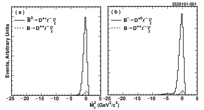
Figure 1: The distribution in $\widetilde{\cal M}_{\nu}^{2}$ for signal (solid histogram), obtained from MC simulation: (left) $\ell-\pi^{+}$ candidates from $\bar{B}^{0}\rightarrow D^{*+}\ell^{-}\bar{\nu}_{\ell}$ {$D^{*+}\rightarrow D^{0}\pi^{+}$}; (right) $\ell-\pi^{0}$ candidates from $B^{-}\rightarrow D^{*0}\ell^{-}\bar{\nu}_{\ell}$ {$D^{*0}\rightarrow D^{0}\pi^{0}$} and $\bar{B}^{0}\rightarrow D^{*+}\ell^{-}\bar{\nu}_{\ell}$ {$D^{*+}\rightarrow D^{+}\pi^{0}$}. The dashed histogram shows the estimated relative contribution from decays $\bar{B}\rightarrow D^{*}\pi\ell^{-}\bar{\nu}_{\ell}$ (correlated background).

where $E_{beam}$ is the beam energy and $E_{\ell}$ and ${\bf{p}}_{\ell}$ are the energy and momentum of the lepton. Correctly identified signal candidates accumulate in the region $\widetilde{\cal M}_{\nu}^{2}>-2.0($GeV${}^{2}/c^{4})$, as can be seen in Figure 1. We define this to be the “peak” region. The “sideband” region, defined as $-25.0<\widetilde{\cal M}_{\nu}^{2}<-4.0$ GeV², is used for estimating backgrounds.

For $\bar{B}^{0}\rightarrow D^{*+}\ell^{-}\bar{\nu}_{\ell}$, leptons are combined with charged pions. Phase space limitations prohibit the decay chain $B^{-}\rightarrow D^{*0}\ell^{-}\bar{\nu}_{\ell}$, $D^{*0}\rightarrow D^{+}\pi^{-}$, leaving only the $\bar{B}^{0}$ decay as a source of leptons which correlate with slow charged pions. In this decay, the lepton must have a charge opposite to that of the slow pion. This combination will be referred to as $\ell-\pi^{+}$.

A lepton may also be combined with a slow neutral pion to reconstruct decays $B\rightarrow D^{*}\ell\bar{\nu}$. In this case both charged and neutral $B$’s contribute to the signal, through the decays $B^{-}\rightarrow D^{*0}\ell^{-}\bar{\nu}_{\ell}(D^{*0}\rightarrow D^{0}\pi^{0})$ and $\bar{B}^{0}\rightarrow D^{*+}\ell^{-}\bar{\nu}_{\ell}(D^{*+}\rightarrow D^{+}\pi^{0})$. Accounting for the respective $D^{*}\rightarrow D\pi$ branching fractions, the reconstructed signal is expected to include $B^{-}\rightarrow D^{*0}\ell^{-}\bar{\nu}_{\ell}$ and $\bar{B}^{0}\rightarrow D^{*+}\ell^{-}\bar{\nu}_{\ell}$ in a ratio of approximately 2:1. The value of $\widetilde{M}_{\nu}^{2}$ is calculated using the measured momentum of the $\pi^{0}\rightarrow\gamma\gamma$ candidate and the known $\pi^{0}$ mass. Such combinations will be referred to as $\ell-\pi^{0}$.

Lepton candidates are required to have momentum between 1.8 GeV/$c$ and 2.5 GeV/$c$. Electrons are identified by using the ratio of the calorimeter energy to track momentum $(E/p)$ and specific ionization $(dE/dx)$ information. Muons are required to penetrate at least five interaction lengths of absorber material. Electrons and muons must fall in the fiducial region $|\cos\theta|<0.707$, where $\theta$ is the polar angle of the track’s momentum vector with respect to the beam axis.

All charged pion candidates are required to have momentum between 90 MeV/$c$ and 220 MeV/$c$ and to be consistent with originating at the interaction point.

Neutral pion candidates are obtained from energy deposits in the cesium iodide electromagnetic calorimeter which do not match the projection of any charged track and are consistent with being electromagnetic showers. Each shower must have energy greater than 50 MeV and be in the good barrel region only ($\cos\theta_{\gamma}<0.71$), where $\theta_{\gamma}$ is the polar angle with respect to the beam axis. The width of the $\gamma\gamma$ invariant mass of $\pi^{0}$’s depends on both the energy and angular resolution of the component photons and averages 5 MeV/$c^{2}$. In order to be able to evaluate the background from random $\gamma\gamma$ pairs (“fake $\pi^{0}$’s”), we consider candidates within a wide mass range, $0.085<M_{\gamma\gamma}<0.185$ GeV/$c^{2}$.

The $\ell-\pi^{+}$ and $\ell-\pi^{0}$ analyses differ mainly in the detection and identification of the soft pion. Because the efficiencies for $\pi^{+}$ and $\pi^{0}$ differ and are momentum-dependent, the overall reconstruction efficiencies will also differ, and their calculation will depend on the decay model used to obtain them, due to differences in momentum distributions. It is reasonable to assume, however, that the isospin-related modes $B^{-}\rightarrow D^{*0}\ell^{-}\bar{\nu}_{\ell}$ and $\bar{B}^{0}\rightarrow D^{*+}\ell^{-}\bar{\nu}_{\ell}$ have the same decay dynamics, and, since the charged and neutral meson masses are nearly equal for both $B$ and $D^{*}$, nearly identical kinematics. The efficiencies to partially reconstruct the two modes should thus differ only due to the momentum-dependent pion efficiencies. We therefore extract the signal yields and ratios in bins of 10 MeV/$c$ in the pion momentum and are then able to make direct model-independent comparisons.

The signal is extracted by counting $\ell-\pi$ candidates which fall in the peak region of $\widetilde{\cal M}_{\nu}^{2}$ (“peak candidates”) and evaluating and subtracting the backgrounds. Backgrounds include contributions from continuum events, leptons or $\pi^{0}$’s that are fake, and real lepton–pion pairs in $B\bar{B}$ events that are not signal. Some of the backgrounds are evaluated using Monte Carlo (MC) simulations, where comparisons with candidates in the sideband region (“sideband candidates”) are used to obtain scaling factors.

The contribution from continuum events is evaluated by analyzing the off-resonance data and scaling to account for the differences in the integrated luminosity and center-of-mass energy. The contribution from fake leptons in $B\bar{B}$ events is estimated by counting continuum-subtracted candidates in which the “lepton” satisfies all criteria except lepton identification, weighted by the fake probability, which is a function of momentum fakprob . After subtracting continuum and fake-lepton backgrounds, the remainder consist of real leptons in combination with soft pion candidates in $B\bar{B}$ events. For $\ell-\pi^{+}$ the numbers are obtained through simple counting. In the case of $\ell-\pi^{0}$ there is additional background from fake $\pi^{0}$’s, formed by random photon combinations. The yields are therefore extracted by fitting the ${\gamma\gamma}$ invariant mass distribution. We first discuss the remaining backgrounds for $\ell-\pi^{+}$ and then return to the treatments of $\ell-\pi^{0}$.

For the $\ell-\pi^{+}$ case the numbers after continuum and fake lepton subtractions are those of peak and sideband candidates consisting of a real lepton in combination with a real soft pion from a $B\bar{B}$ event. The remaining backgrounds are of two general types. Candidates formed from the lepton and soft pion from the $D^{*}$ in decays of the type $\bar{B}\rightarrow D^{*}\pi\ell^{-}\bar{\nu}_{\ell}(D^{*}\rightarrow D^{0}\pi)$ will accumulate near $\widetilde{\cal M}_{\nu}^{2}=0$ and are difficult to distinguish from signal. We define this type as “correlated background.” All other combinations, where the pion is not the daughter of a $D^{*}$ from the same $B$ meson as the lepton, are defined as “uncorrelated background.”

We use the CLEO MC simulation, the decay model of Goity and Robertsgoityroberts , and measured branching fractions to estimate the contribution of correlated background. The $D^{*}\pi$ combinations include three $D^{**}$ resonances, as well as non-resonant production. The total rate is set to match the ALEPH measurementlepd2s , ${\cal B}(b\rightarrow\bar{B})\times{\cal B}(\bar{B}\rightarrow D^{*+}\pi^{-}\ell^{-}\nu X)=(4.73\pm 0.77\pm 0.55)\times 10^{-3}$. By isospin symmetry, we assume that $B\rightarrow D^{*+}\pi^{0}\ell^{+}\nu X$ contributes additionally at half of this rate, and that the rates to $D^{*0}$ are equal to the corresponding rates for $D^{*+}$. We then use the ALEPH value ${\cal B}(b\rightarrow\bar{B})=(37.8\pm 2.2)\%$ to obtain ${\cal B}(B\rightarrow D^{*-/0}\pi\ell^{+}\nu X)=(1.88\pm 0.39)\%$, where the statistical and systematic errors have been added in quadrature. The resulting numbers of candidates are scaled to the integrated luminosity of the data and subtracted directly from the peak and sideband samples. The $D^{**}$ contributions to the peak are small, due to the high lepton momentum requirement imposed in this analysis. We find that this background comprises $(2.8\pm 0.2)$% of the net signal. The contributions to the sideband are much smaller.

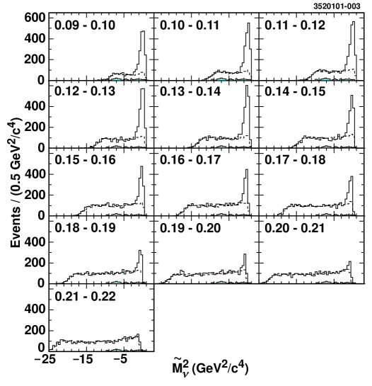
Figure 2: Distributions in $\widetilde{\cal M}_{\nu}^{2}$ for the decay $\bar{B}^{0}\rightarrow D^{*+}\ell^{-}\bar{\nu}_{\ell}$, for 10 MeV/c bins of pion momentum. The plot shows right sign data, with continuum and fake lepton contributions subtracted (solid histograms), uncorrelated background (dashed), and correlated backround (black filled) estimated by Monte Carlo.

The uncorrelated background is estimated via MC simulation. We reconstruct $\ell-\pi^{+}$ candidates in 17.5 million generic MC $B\bar{B}$ events, excluding signal and correlated background. To obtain a data/MC scaling factor, ratios of sideband candidates in data and MC are found in all momentum bins and the set of ratios is fitted to a single value. The numbers of peak candidates from MC are multiplied by this factor to obtain the contributions of uncorrelated background. Figure 2 displays the $\widetilde{\cal M}_{\nu}^{2}$ distributions in each pion momentum bin of data after continuum and fake subtractions, correlated background (MC), and uncorrelated background (MC, scaled). The agreement between MC and data of the uncorrelated background in the sideband region is excellent. Peak candidates in excess of the evaluated backgrounds comprise our signal.

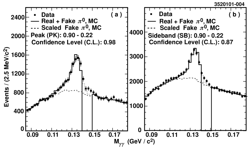
Figure 3: Fit of $M_{\gamma\gamma}$ distribution comprising $\ell-\pi^{0}$ peak (left) and sideband (right) tags. The region 0.140-0.150 GeV/c² is omitted from the fit in this and all other fits of $M_{\gamma\gamma}$ described in this report.

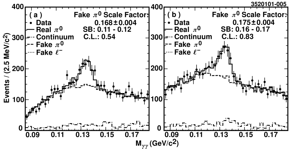
Figure 4: Fits of $M_{\gamma\gamma}$ to MC-generated real and fake $\pi^{0}$ distributions for $\ell-\pi^{0}$ sideband candidates, 0.11-0.12 GeV/c² (left) and 0.16-0.17 GeV/c² (right). The fake lepton contributions are not visible in this plot. This fit was used to determine the data/MC scaling factor for fake $\pi^{0}$’s.

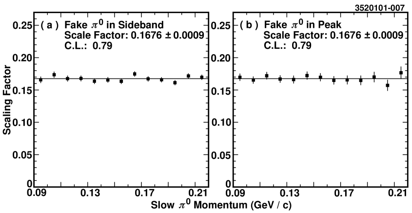
Figure 6: Fit of fake $\pi^{0}$ scaling factors to a constant. Scaling factors are plotted as a function of momentum for sideband (left) and peak (right) candidates and fitted simultaneously to a single constant.

The procedure applied to $\ell-\pi^{0}$ is similar in concept, but instead of simple counting we fit the $\gamma\gamma$ invariant mass distributions. After the direct subtractions of continuum and fake leptons, the remaining distributions contain in addition to the backgrounds discussed for the $\ell-\pi^{+}$ (correlated and uncorrelated background) the contribution from $B\bar{B}$ events where the lepton is real and the pion is fake. The correlated background is estimated and subtracted first. In the case of $\ell-\pi^{0}$ there are contributions from modes containing both charged and neutral $D^{*}$. As with $\ell-\pi^{+}$, the contributions are calculated based on the branching fraction measured at LEP and MC simulation. We find that the correlated background comprises $(2.5\pm 0.9)$% of the net signal in the peak region. The contribution in the sideband region, which is much smaller, is also calculated and subtracted. We then determine the contribution of fake $\pi^{0}$. The resulting $\gamma\gamma$ invariant mass distributions are fitted to a sum of real and fake $\pi^{0}$ distributions generated via MC simulation. In the fit we exclude the region $0.14<M_{\gamma\gamma}c^{2}<0.15$ GeV because the simulated $\pi^{0}$ signal in this region does not show good agreement with data. Although this disagreement is not apparent in the individual pion momentum bins, due to insufficient statistics, it is revealed when we fit to a distribution that is summed over all bins (Figure 3). We find that the fake $\pi^{0}$ background is well simulated by MC in that the fits all have good confidence and that the data/MC scaling factors are consistent with being a single constant over all $\pi^{0}$ momenta for both sideband and peak distributions. Figures 4 and 5 show examples of fit results. Figure 6 shows results from a fit of all of the scaling factors to a single constant. That fit gives a confidence level of 80% and a scaling factor of $0.1676\pm 0.0009$, very close to the ratio of the numbers of $B\bar{B}$ events in data and MC ($0.1667\pm 0.0001$). We use this fitted value to calculate the amount of fake $\pi^{0}$ in each distribution considered.

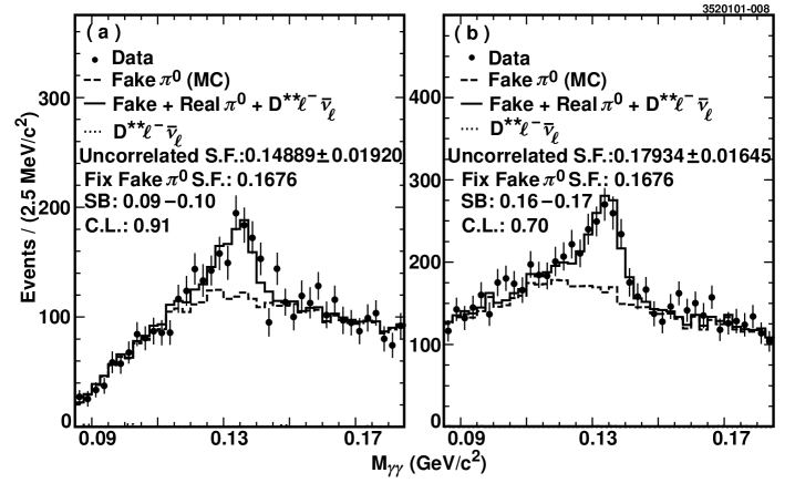
Figure 7: Fits of $M_{\gamma\gamma}$ for sideband candidates, to determine data/MC normalization of uncorrelated background. The fake normalization is fixed. The correlated background from $D^{**}\ell\nu$ is not visible in this plot. Shown are plots for two bins of $\pi^{0}$ momentum.

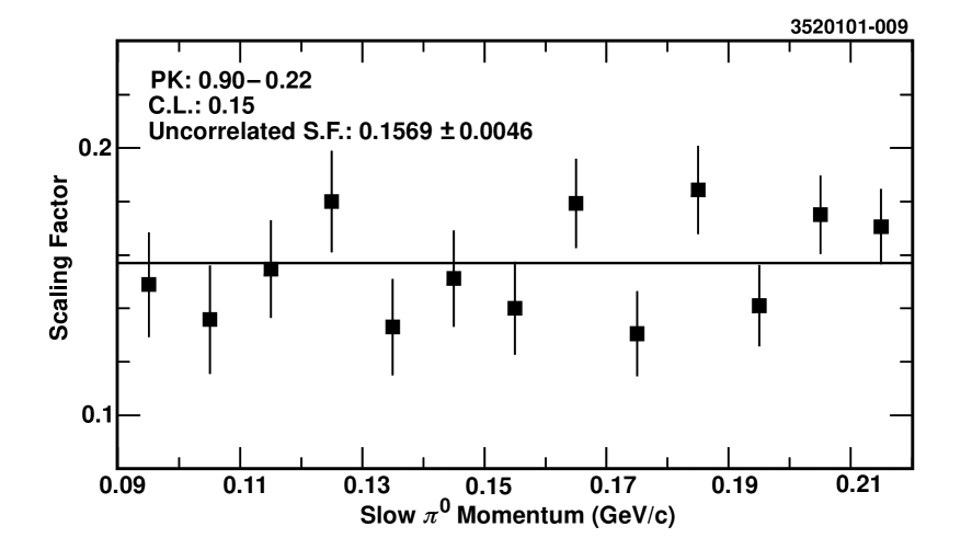
Figure 8: Fit of data/MC scaling factors for uncorrelated background. Scaling factors obtained by fitting in momentum bins are fitted to a single constant.

The sideband candidates remaining after the above background subtractions consist of uncorrelated background. For each momentum bin, the associated $M_{\gamma\gamma}$ distribution is fitted to the corresponding MC simulation to obtain a data/MC scaling factor. Figure 7 shows two plots with typical fit results. A fit of the resulting scaling factors (Figure 8) shows good consistency with the hypothesis of a single constant scaling factor. The fitted value of $0.157\pm 0.005$ is used as the overall scaling factor to estimate the uncorrelated background in the peak region.

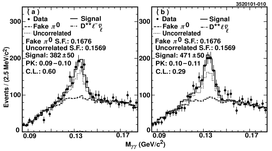
Figure 9: Fits of $M_{\gamma\gamma}$ for peak candidates, to determine signal yields. The fake, correlated, and uncorrelated background normalizations are fixed. Shown are plots for two bins of $\pi^{0}$ momentum.

We fit the remaining $M_{\gamma\gamma}$ distribution of peak candidates in each momentum bin to obtain the signal yield. Two examples are shown in Figure 9.

III.1 Signal Yields

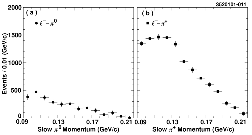
Figure 10: Yield in data of partially reconstructed signal in $\ell-\pi^{0}$(left) and $\ell-\pi^{+}$ (right) as a function of $\pi$ momentum. Distributions are not corrected for reconstruction efficiency.

After all background subtractions listed above, a total of $11,262\pm 164$ $\ell-\pi^{+}$ and $2,686\pm 142$ $\ell-\pi^{0}$ remain as signal. Figure 10 shows the yields as a function of pion momentum.

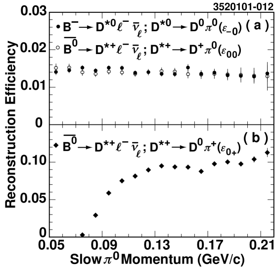
Figure 11: Efficiencies for reconstruction of decays via partial reconstruction, as a function of $\pi$ momentum: $\ell-\pi^{0}$ (top) and $\ell-\pi^{+}$ (bottom) analysis.

To obtain reconstruction efficiencies, we generated events containing $B\rightarrow D^{*}\ell\bar{\nu}(D^{*}\rightarrow D\pi)$ using the model of Scora and Isgurisgw2 (ISGW2). The events were passed through a full GEANT-based detector simulation and offline analysis. We perform the analysis on tagged signal candidates. Figure 11 shows the resulting efficiency as a function of pion momentum for both $\ell-\pi^{+}$ and $\ell-\pi^{0}$ analyses. The efficiencies for $\ell-\pi^{0}$ reconstruction of $\bar{B}^{0}\rightarrow D^{*+}\ell^{-}\bar{\nu}_{\ell}$ and $\bar{B}^{-}\rightarrow D^{*0}\ell^{-}\bar{\nu}_{\ell}$ are expected to be equal, and since the MC result is consistent with this expectation, it is assumed to be the case.

IV Relationship of measurement to decay rates

The numbers of reconstructed $\ell-\pi^{+}$ and $\ell-\pi^{0}$ signal, $N_{+}$ and $N_{0}$, have the following relationships to the branching fractions:

$$N_{+} =$$ (2)

$$2\times 2\times N_{B\bar{B}}f_{00}\times\epsilon_{0+}\times{\cal B}(\bar{B}^{0}\rightarrow D^{*+}\ell^{-}\bar{\nu}_{\ell})\times{\cal B}(D^{*+}\rightarrow D^{0}\pi^{+}),$$

$${\rm and}$$ (3)

$$N_{0} =$$ (4)

$$2\times 2\times N_{B\bar{B}}f_{+-}\times\epsilon_{-0}\times{\cal B}(B^{-}\rightarrow D^{*0}\ell^{-}\bar{\nu}_{\ell})\times{\cal B}(D^{*0}\rightarrow D^{0}\pi^{0})$$

$$+ 2\times 2\times N_{B\bar{B}}f_{00}\times\epsilon_{00}\times{\cal B}(\bar{B}^{0}\rightarrow D^{*+}\ell^{-}\bar{\nu}_{\ell})\times{\cal B}(D^{*+}\rightarrow D^{+}\pi^{0}),$$

where $f_{00}$ $(f_{+-})$ is the fraction of neutral (charged) B mesons in $\Upsilon(4S)$ events, and $\epsilon_{0+}$, $\epsilon_{-0}$, and $\epsilon_{00}$ are the reconstruction efficiencies for the respective $B\rightarrow D^{*}\ell\nu(D^{*}\rightarrow D\pi)$ modes. Two factors of 2 enter in these expressions because each $B\bar{B}$ event contains two B mesons, and we add the signals for electrons and muons. Solving for the branching fractions,

$${\cal B}(\bar{B}^{0}\rightarrow D^{*+}\ell^{-}\bar{\nu}_{\ell}) = \frac{N_{+}}{4N_{B\bar{B}}f_{00}\epsilon_{0+}{\cal B}(D^{*+}\rightarrow D^{0}\pi^{+})}$$ (5)

$${\cal B}(B^{-}\rightarrow D^{*0}\ell^{-}\bar{\nu}_{\ell}) = \frac{N_{0}-4N_{B\bar{B}}f_{00}\epsilon_{00}{\cal B}(\bar{B}^{0}\rightarrow D^{*+}\ell^{-}\bar{\nu}_{\ell}){\cal B}(D^{*+}\rightarrow D^{+}\pi^{0})}{4N_{B\bar{B}}f_{+-}\epsilon_{-0}{\cal B}(D^{*0}\rightarrow D^{0}\pi^{0})}$$ (6)

$$= \frac{N_{0}-N_{+}{\epsilon_{00}{\cal B}(D^{*+}\rightarrow D^{+}\pi^{0})\over\epsilon_{0+}{\cal B}(D^{*+}\rightarrow D^{0}\pi^{+})}}{4N_{B\bar{B}}f_{+-}\epsilon_{-0}{\cal B}(D^{*0}\rightarrow D^{0}\pi^{0})}$$

Dividing equation (6) by equation (5), assuming that $\epsilon_{-0}=\epsilon_{00}$, and defining $n\equiv{N_{+}\epsilon_{00}\over N_{0}\epsilon_{0+}}$, we get

$${{\cal B}(B^{-}\rightarrow D^{*0}\ell^{-}\bar{\nu}_{\ell})\over{\cal B}(\bar{B}^{0}\rightarrow D^{*+}\ell^{-}\bar{\nu}_{\ell})} = {f_{00}[{\cal B}(D^{*+}\rightarrow D^{0}\pi^{+})-n{\cal B}(D^{*+}\rightarrow D^{+}\pi^{0})]\over nf_{+-}{\cal B}(D^{*0}\rightarrow D^{0}\pi^{0})},\ {\rm and}$$ (7)

$$\alpha\equiv{f_{+-}\over f_{00}}{{\cal B}(B^{-}\rightarrow D^{*0}\ell^{-}\bar{\nu}_{\ell})\over{\cal B}(\bar{B}^{0}\rightarrow D^{*+}\ell^{-}\bar{\nu}_{\ell})} \equiv {{\cal B}(D^{*+}\rightarrow D^{0}\pi^{+})-n{\cal B}(D^{*+}\rightarrow D^{+}\pi^{0})\over n{\cal B}(D^{*0}\rightarrow D^{0}\pi^{0})}.$$ (8)

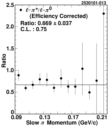
Figure 12: Efficiency-corrected ratio of $\ell-\pi^{+}$ to $\ell-\pi^{0}$ candidates in bins of $\pi$ momentum. The values are fitted to a constant.

Although it is implied in the above equations that the ratio $n$ is a ratio of total rates, it is equal to the ratio of rates over any given restricted kinematic region, as long as the kinematics of the decays are the same. We thus take the ratio of the $\ell-\pi^{+}$ to $\ell-\pi^{0}$ signals as a function of pion momentum, correct for the reconstruction efficiencies in each bin to obtain $n$, and fit to a constant. The fit yields an overall value $n=0.669\pm 0.037$ (Figure 12). Using this value and the $D^{*}$ branching fractions shown in Table 1, we obtain $\alpha=1.136\pm 0.090$, where the error is statistical only.

V Systematic Errors

The systematic uncertainty on $\alpha$ is due to the uncertainty in determining the ratio $n$ and uncertainties in the $D^{*}$ branching fractions. The reconstructions $\ell-\pi^{0}$ and $\ell-\pi^{+}$ have many features in common and therefore many shared systematic errors which cancel at least partially in taking the ratio. The principal difference between the two is in the reconstruction of the pions.

We first discuss the uncertainties from lepton detection/identification and background subtractions that are common to both reconstructions. The uncertainty on the continuum subtraction is obtained by changing the scaling factor up and down by 3%. The uncertainty on the lepton fake probability is 30%. The systematic uncertainty on the lepton identification efficiency has been determined to be $2.5\%$mssthesis . The systematic uncertainties from each of these sources is estimated by varying the affected quantity and observing the shift of the result. These errors cancel at least partially in taking the ratio $n$.

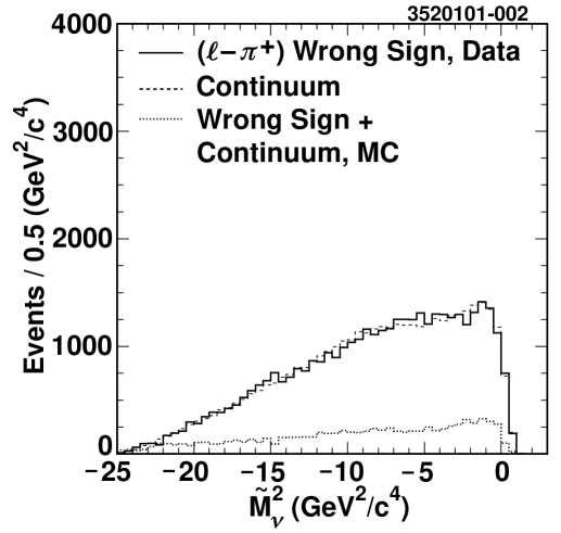
Figure 13: The distribution in $\widetilde{\cal M}_{\nu}^{2}$ for wrong-sign $\ell-\pi^{+}$ candidates, data on resonance (solid histogram), data off resonance, scaled (dotted), and MC normalized to data in the sideband region (dashed–dotted).

The estimation of uncorrelated background depends on accurate modeling of the peak/sideband ratio by MC. The overall $\widetilde{\cal M}_{\nu}^{2}$ distribution of the uncorrelated background is dominated by phase space, i.e., a hard lepton and soft pion distributed isotropically will produce a distribution similar to that shown. However, because this analysis has high statistical precision, we are somewhat sensitive to the finer details of the Monte Carlo $B$ decay generator. A simple overall test of its reliability is the counting of wrong sign ($\ell^{\pm}-\pi^{\pm}$) candidates, where no signal is expected. An analysis identical to that performed with right sign $\ell-\pi^{+}$ yields a signal of $-91\pm 117$, consistent with zero. The wrong sign distribution of $\widetilde{\cal M}_{\nu}^{2}$ in data and MC simulation are shown in Figure 13. We take the absolute sum of the “signal” and statistical error, $\left|{-91}\right|+117=208$, as an estimate of the systematic uncertainty due to modeling. This is 3.3% of the number of wrong sign peak candidates after continuum and fake subtractions, so we take 3.3% as the fractional uncertainty on the uncorrelated background in the right sign. This translates to 1.9% of the net signal in $\ell-\pi^{+}$. For the $\ell-\pi^{0}$, the corresponding uncertainty is 2.0% of the net signal. Although these two uncertainties are believed to be largely correlated, and should cancel at least partially in taking the ratio, we conservatively take the error on $n$ to be equal to the larger one, 2.0%.

To estimate the uncertainty due to our lack of knowledge of the $B$ semileptonic decays to $D^{*}\pi$, we vary both the total branching fraction and the mix of resonant and non-resonant contributions to $D^{*}\pi$. The branching fraction, which we took to be $(1.88\pm 0.39)$% for each $D^{*}$ charge, averaged over $B$ charges as explained earlier, is varied up and down by the amount of the error, holding fixed the relative contributions of the different modes. We recorded excursions of 0.5% and 0.3% for $\ell-\pi^{0}$ and $\ell-\pi^{+}$, respectively. We also allow each mode in turn to saturate the rate and take the maximum excursion of the result as a systematic uncertainty. We thus obtain errors of 0.8%, 1.4%, and 1.0%, for $\ell-\pi^{0}$, $\ell-\pi^{+}$, and $n$.

The systematic uncertainty on tracking efficiency for slow charged pions has been measured in a previous CLEO analysisbarish to be 5%. The uncertainty on the efficiency ratio of slow neutral pions to slow charged pions was determined to be 7%. As the absolute efficiency for neutral pion reconstruction is determined by the charged pion efficiency and the ratio, the quadratic sum of their uncertainties gives the systematic uncertainty of $8.6\%$barish on the neutral pion efficiency.

To estimate the systematic error on the evaluation of fake $\pi^{0}$’s in $\ell-\pi^{0}$, we vary the fake scaling factor up and down by the amount of its statistical error and repeat the analysis. We take the maximum excursion of 1.6% to be the systematic uncertainty from this source. We also repeat the analysis without excluding the $\gamma\gamma$ mass region $0.014-0.015$ GeV/c² and find that this shifts the result by 0.7%. We add the two numbers quadratically to get a systematic error on the $\pi^{0}$ fit of 1.7%.

We find the total systematic errors to be $9.4\%$ for $\ell-\pi^{0}$, ${6.1}\%$ for $\ell-\pi^{+}$, and 7.6% for $n$. This results in an uncertainty of 10.9% on $\alpha$. The additional uncertainty from the $D^{*}$ branching fractions is 6.3%. All the systematic uncertainties are summarized in Table 2.

VI Summary and Conclusions

By measuring the ratio of partially reconstructed $B\rightarrow D^{*}\ell\nu$ decays in the $\ell-\pi^{+}$ and $\ell-\pi^{0}$ channels as a function of pion momentum, we obtain a measurement of the ratio

$$\frac{f_{+-}}{f_{00}}\frac{\tau_{+}}{\tau_{0}}=1.136\pm 0.090\pm 0.143.$$

This result is in good agreement with published CLEO values (Table 3).

Using the ratio of $B^{+}$ and $B^{0}$ lifetimes from a recent world averagepdg ,

$$\frac{\tau_{+}}{\tau_{0}}=1.074\pm 0.028,$$

we obtain the ratio of the charged and neutral $B$ meson production at the $\Upsilon(4S)$ resonance:

$$\frac{f_{+-}}{f_{00}}=1.058\pm 0.084\pm 0.115\pm 0.067\pm 0.028$$

where the first error is statistical, the second is systematic on n, the third is due to the uncertainty on the $D^{*}$ branching fractions, and the fourth is due to the uncertainty on the $B$ lifetime ratio. We add the systematic errors quadratically to obtain

$$\frac{f_{+-}}{f_{00}}=1.058\pm 0.084\pm 0.136.$$

Table 1: Branching fractions of $D^{*}\rightarrow D\pi$

MODE	Branching Fraction	reference
$D^{*+}\rightarrow D^{0}\pi^{+}$	$(67.6\pm 0.8)\%$	Dstbr1
$D^{*+}\rightarrow D^{+}\pi^{0}$	$(30.7\pm 0.7)\%$	Dstbr1
$D^{*0}\rightarrow D^{0}\pi^{0}$	$(61.9\pm 2.9)\%$	pdg

Table 2: Summary of systematic errors (%).

Source	$\ell-\pi^{0}$	$\ell-\pi^{+}$	$n$	$\alpha$
Continuum subtraction	$0.2$	$0.2$	0.2	0.3
Fake leptons	$0.5$	$0.5$	$0.5$	$0.7$
Uncorrelated background	$2.0$	$1.9$	2.0	2.9
$D^{**}$ background	$0.8$	$1.4$	1.0	1.4
Fake $\pi^{0}$ subtraction	$1.7$	–	1.7	2.4
$\pi$ efficiency	$8.6$	$5.0$	7.0	10.0
Lepton ID efficiency	$2.5$	$2.5$	–	–
$D^{*}$ Branching Fraction	$-$	$-$	$-$	6.3
Total	$9.4$	$6.1$	7.6	12.6

Table 3: Other CLEO measurements of $\frac{f_{+-}}{f_{00}}\frac{\tau_{+}}{\tau_{0}}$

Mode	$\frac{f_{+-}}{f_{00}}\frac{\tau_{+}}{\tau_{0}}$
$B\rightarrow D^{*}\ell\bar{\nu}$barish	$1.14\pm 0.14\pm 0.13$
$B\rightarrow\psi K^{(*)}$ eigen	$1.11\pm 0.07\pm 0.04$

VII Acknowledgements

We gratefully acknowledge the effort of the CESR staff in providing us with excellent luminosity and running conditions. M. Selen thanks the PFF program of the NSF and the Research Corporation, and A.H. Mahmood thanks the Texas Advanced Research Program. This work was supported by the National Science Foundation, and the U.S. Department of Energy.

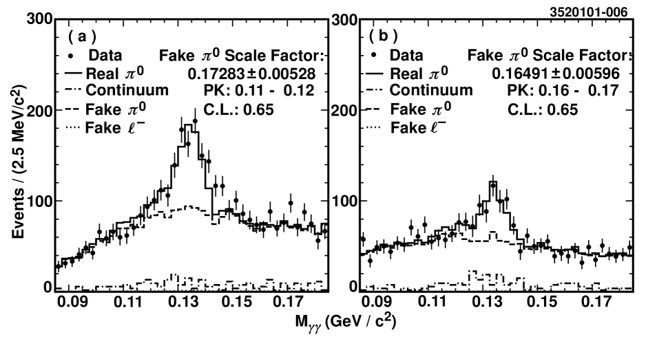
Figure 5: Plots as described in Figure 4, for peak candidates.

References

- (1) P. Lepage, Phys. Rev. D42, 3251 (1990); D. Atwood and W. Marciano, Phys. Rev. D41, 1736 (1990).
- (2) M. Artuso et al. (CLEO), Phys. Lett. B 399, 321 (1997).
- (3) M.S. Saulnier, Ph.D. thesis, Harvard University, 1995 (unpublished); I. C. Lai, Ph.D. thesis, Virginia Tech, 1999 (unpublished).
- (4) Y. Kubota et al., Nuclear Instrum. Methods A320, 66 (1992).
- (5) G. Fox and S. Wolfram, Phys. Rev. Lett. 41 1581 (1978).
- (6) R. Wang, Ph.D. thesis, University of Minnesota, 1994 (unpublished).
- (7) J.L. Goity and W. Roberts, Phys. Rev D 51, 3459 (1995)
- (8) D. Buskulic et al., Z. Phys. C73, 601 (1997); P. Abreu et al., Phys. Lett. B475, 407 (2000).
- (9) D. Scora and N. Isgur, Phys. Rev. D 52, 2783 (1995); N. Isgur, D. Scora, B. Grinstein, and M.B. Wise, Phys. Rev D 39, 799 (1989).
- (10) B. Barish et al. (CLEO), Phys. Rev. D 51, 1014 (1995).
- (11) D. E. Groom et al., The European Physical Journal C15, 1 (2000) and 2001 off-year partial update for the 2002 edition available on the PDG WWW pages (URL: http://pdg.lbl.gov/).
- (12) J. Bartelt et al. (CLEO), Phys. Rev. Lett. 80, 3919 (1998).
- (13) J.P. Alexander et al. (CLEO), Phys. Rev. Lett. 86, 2737 (2001).