Abstract

This report describes an observation of mixing-induced $CP$ violation and a measurement of the $CP$ violation parameter, $\sin 2\phi_{1}$, with the Belle detector at the KEKB asymmetric $e^{+}e^{-}$ collider. Using a data sample of 29.1 fb^-1 recorded on the $\Upsilon(4S)$ resonance that contains 31.3 million $B\overline{B}$ pairs, we reconstruct decays of neutral $B$ mesons to the following $CP$ eigenstates: $J/\psi K_{S}^{0}$, $\psi(2S)K_{S}^{0}$, $\chi_{c1}K_{S}^{0}$, $\eta_{c}K_{S}^{0}$, $J/\psi K_{L}^{0}$ and $J/\psi K^{*0}$. The flavor of the accompanying $B$ meson is identified by combining information from primary and secondary leptons, $K^{\pm}$ mesons, $\Lambda$ baryons, slow and fast pions. The proper-time interval between the two $B$ meson decays is determined from the distance between the two decay vertices measured with a silicon vertex detector.

The result $\sin 2\phi_{1}=0.99\pm 0.14({\rm stat})\pm 0.06({\rm syst})$ is obtained by applying a maximum likelihood fit to the 1137 candidate events. We conclude that there is large $CP$ violation in the neutral $B$ meson system. A zero value for $\sin 2\phi_{1}$ is ruled out by more than six standard deviations.

KEK Preprint 2001-172
                                                                                                                        Belle Preprint 2002-6

The Belle Collaboration K. Abe⁹, K. Abe⁴³, R. Abe³¹, T. Abe⁴⁴, I. Adachi⁹, Byoung Sup Ahn¹⁷, H. Aihara⁴⁵, M. Akatsu²⁴, Y. Asano⁵⁰, T. Aso⁴⁹, T. Aushev¹⁴, A. M. Bakich⁴⁰, Y. Ban³⁵, E. Banas²⁹, S. Behari⁹, P. K. Behera⁵¹, A. Bondar², A. Bozek²⁹, M. Bračko^22,15, T. E. Browder⁸, B. C. K. Casey⁸, P. Chang²⁸, Y. Chao²⁸, B. G. Cheon³⁹, R. Chistov¹⁴, S.-K. Choi⁷, Y. Choi³⁹, L. Y. Dong¹², J. Dragic²³, A. Drutskoy¹⁴, S. Eidelman², V. Eiges¹⁴, Y. Enari²⁴, C. W. Everton²³, F. Fang⁸, C. Fukunaga⁴⁷, M. Fukushima¹¹, N. Gabyshev⁹, A. Garmash^2,9, T. Gershon⁹, B. Golob^21,15, A. Gordon²³, H. Guler⁸, R. Guo²⁶, J. Haba⁹, H. Hamasaki⁹, K. Hanagaki³⁶, F. Handa⁴⁴, K. Hara³³, T. Hara³³, N. C. Hastings²³, H. Hayashii²⁵, M. Hazumi⁹, E. M. Heenan²³, I. Higuchi⁴⁴, T. Higuchi⁴⁵, T. Hojo³³, T. Hokuue²⁴, Y. Hoshi⁴³, S. R. Hou²⁸, W.-S. Hou²⁸, S.-C. Hsu²⁸, H.-C. Huang²⁸, T. Igaki²⁴, T. Iijima⁹, H. Ikeda⁹, K. Inami²⁴, A. Ishikawa²⁴, H. Ishino⁴⁶, R. Itoh⁹, H. Iwasaki⁹, Y. Iwasaki⁹, D. J. Jackson³³, H. K. Jang³⁸, H. Kakuno⁴⁶, J. H. Kang⁵⁴, J. S. Kang¹⁷, P. Kapusta²⁹, N. Katayama⁹, H. Kawai³, H. Kawai⁴⁵, Y. Kawakami²⁴, N. Kawamura¹, T. Kawasaki³¹, H. Kichimi⁹, D. W. Kim³⁹, Heejong Kim⁵⁴, H. J. Kim⁵⁴, H. O. Kim³⁹, Hyunwoo Kim¹⁷, S. K. Kim³⁸, T. H. Kim⁵⁴, K. Kinoshita⁵, H. Konishi⁴⁸, S. Korpar^22,15, P. Križan^21,15, P. Krokovny², R. Kulasiri⁵, S. Kumar³⁴, A. Kuzmin², Y.-J. Kwon⁵⁴, J. S. Lange⁶, G. Leder¹³, S. H. Lee³⁸, A. Limosani²³, D. Liventsev¹⁴, R.-S. Lu²⁸, J. MacNaughton¹³, G. Majumder⁴¹, F. Mandl¹³, D. Marlow³⁶, T. Matsuishi²⁴, S. Matsumoto⁴, T. Matsumoto²⁴, Y. Mikami⁴⁴, W. Mitaroff¹³, K. Miyabayashi²⁵, Y. Miyabayashi²⁴, H. Miyake³³, H. Miyata³¹, G. R. Moloney²³, S. Mori⁵⁰, T. Mori⁴, A. Murakami³⁷, T. Nagamine⁴⁴, Y. Nagasaka¹⁰, Y. Nagashima³³, T. Nakadaira⁴⁵, E. Nakano³², M. Nakao⁹, J. W. Nam³⁹, Z. Natkaniec²⁹, K. Neichi⁴³, S. Nishida¹⁸, O. Nitoh⁴⁸, S. Noguchi²⁵, T. Nozaki⁹, S. Ogawa⁴², T. Ohshima²⁴, T. Okabe²⁴, S. Okuno¹⁶, S. L. Olsen⁸, W. Ostrowicz²⁹, H. Ozaki⁹, P. Pakhlov¹⁴, H. Palka²⁹, C. S. Park³⁸, C. W. Park¹⁷, H. Park¹⁹, K. S. Park³⁹, L. S. Peak⁴⁰, J.-P. Perroud²⁰, M. Peters⁸, L. E. Piilonen⁵², E. Prebys³⁶, J. L. Rodriguez⁸, F. Ronga²⁰, M. Rozanska²⁹, K. Rybicki²⁹, H. Sagawa⁹, Y. Sakai⁹, M. Satapathy⁵¹, A. Satpathy^9,5, O. Schneider²⁰, S. Schrenk⁵, C. Schwanda^9,13, S. Semenov¹⁴, K. Senyo²⁴, M. E. Sevior²³, H. Shibuya⁴², B. Shwartz², V. Sidorov², J. B. Singh³⁴, S. Stanič⁵⁰, A. Sugi²⁴, A. Sugiyama²⁴, K. Sumisawa⁹, T. Sumiyoshi⁹, K. Suzuki⁹, S. Suzuki⁵³, S. Y. Suzuki⁹, H. Tajima⁴⁵, T. Takahashi³², F. Takasaki⁹, M. Takita³³, K. Tamai⁹, N. Tamura³¹, J. Tanaka⁴⁵, M. Tanaka⁹, G. N. Taylor²³, Y. Teramoto³², S. Tokuda²⁴, M. Tomoto⁹, T. Tomura⁴⁵, S. N. Tovey²³, K. Trabelsi⁸, W. Trischuk^36,†, T. Tsuboyama⁹, T. Tsukamoto⁹, S. Uehara⁹, K. Ueno²⁸, Y. Unno³, S. Uno⁹, Y. Ushiroda⁹, S. E. Vahsen³⁶, K. E. Varvell⁴⁰, C. C. Wang²⁸, C. H. Wang²⁷, J. G. Wang⁵², M.-Z. Wang²⁸, Y. Watanabe⁴⁶, E. Won³⁸, B. D. Yabsley⁹, Y. Yamada⁹, M. Yamaga⁴⁴, A. Yamaguchi⁴⁴, H. Yamamoto⁴⁴, T. Yamanaka³³, Y. Yamashita³⁰, M. Yamauchi⁹, J. Yashima⁹, M. Yokoyama⁴⁵, Y. Yuan¹², Y. Yusa⁴⁴, H. Yuta¹, C. C. Zhang¹², J. Zhang⁵⁰, Y. Zheng⁸, V. Zhilich², and D. Žontar⁵⁰

I Introduction

The phenomenon of $CP$ violation is one of the major unresolved issues in our understanding of particle physics today. In 1973, Kobayashi and Maskawa (KM) proposed a model where $CP$ violation is accommodated as an irreducible complex phase in the weak-interaction quark mixing matrix[1], which is defined as

$$\left(\begin{array}[]{ccc}V_{ud}&V_{us}&V_{ub}\\ V_{cd}&V_{cs}&V_{cb}\\ V_{td}&V_{ts}&V_{tb}\end{array}\right),$$ (1)

where the nontrivial complex phases are conventionally assigned to the furthest off-diagonal elements $V_{ub}$ and $V_{td}$. Unitarity of this CKM matrix (Cabibbo-Kobayashi-Maskawa matrix) implies that $\Sigma_{i}V_{ij}V_{ik}^{*}=\delta_{jk}$, which gives the following relation involving $V_{ub}$ and $V_{td}$:

$$V_{ud}V_{ub}^{*}+V_{cd}V_{cb}^{*}+V_{td}V_{tb}^{*}=0.$$ (2)

This expression can be visualized as a closed triangle in the complex plane as shown in Fig. 1.

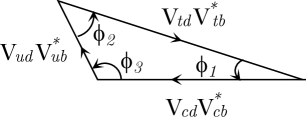
FIG. 1.: The unitarity triangle relevant to $B$ decays. Angles of the triangle arise from the KM phase.

The three interior angles of the unitarity triangle originate from the non-vanishing $CP$-violating phase (the KM phase) and are defined as[2]:

$$\phi_{1} \equiv \pi-{\rm arg}({-V_{td}V_{tb}^{*}}/{-V_{cd}V_{cb}^{*}}),$$ (3)

$$\phi_{2} \equiv {\rm arg}({V_{td}V_{tb}^{*}}/{-V_{ud}V_{ub}^{*}}),$$ (4)

$$\phi_{3} \equiv {\rm arg}({V_{ud}V_{ub}^{*}}/{-V_{cd}V_{cb}^{*}}).$$ (5)

The bold ansatz of Kobayashi and Maskawa required the existence of six quarks at a time when only the $u$, $d$ and $s$ quarks were known. The subsequent discoveries of the $c$, $b$ and $t$ quarks as well as the consistency with the $CP$ violation observed in the neutral kaon system led to the incorporation of the KM mechanism as an essential component of the Standard Model (SM).

In 1980, Sanda, Bigi and Carter pointed out that the KM model contained the possibility of sizable $CP$-violating asymmetries in certain neutral $B$ meson decays [3]. The subsequent observation of a long $b$ quark lifetime[4] and a large mixing in the neutral $B$ meson system[5] indicated that it would be feasible to measure $CP$ violation in $B$ meson decays at an asymmetric $e^{+}e^{-}$ collider at the $\Upsilon(4S)$ energy.

Until recently the only observation of $CP$ violation was in the neutral kaon system, where the interpretation of results is complicated due to large corrections from the strong interaction. By contrast, these corrections are absent or very small for the aforementioned $CP$ violation in the neutral $B$ meson system. Thus its measurement can be used to over-constrain and test the consistency of the SM.

A pair of neutral $B$ mesons created in the decay $\Upsilon(4S)\rightarrow B^{0}{\overline{B}{}^{0}}$ is in a state with $C=-1$ at the time of production ($t=0$), where $C$ denotes the charge conjugation. Although oscillation then starts, the state preserves the $C$ odd configuration and is not allowed to be $B^{0}B^{0}$ or ${\overline{B}{}^{0}}{\overline{B}{}^{0}}$. The time evolution of the pair is given by

$$|\Psi(t)\rangle = e^{-t/\tau_{B^{0}}}|\Psi(t=0)\rangle,$$ (6)

$$|\Psi(t=0)\rangle = \frac{1}{\sqrt{2}}\left[|B^{0}(\vec{k}){\overline{B}{}^{0}}(-\vec{k})\rangle-|B^{0}(-\vec{k}){\overline{B}{}^{0}}(\vec{k})\rangle\right],$$ (7)

where $\vec{k}$ and $-\vec{k}$ are the $B$ mesons’ momenta in the $\Upsilon(4S)$ rest frame. This coherence is preserved until one $B$ meson decays. Hence, if we can determine the flavor and the decay time $t_{\rm tag}$ of one of the $B$ mesons decaying into a final state $f_{\rm tag}$, we are able to determine the time-dependent decay amplitude of the other $B$ at any time $t$ as a function of the time difference $t-t_{\rm tag}$. We consider the case where the other $B$ meson decays at $t=t_{CP}$ to a $CP$ eigenstate, $f_{CP}$. When the decay is dominated by a single transition amplitude, the following formulae for the decay rates hold to a good approximation[3]:

$$R(B^{0}\rightarrow f_{CP};\;\Delta t) = e^{-|\Delta t|/\tau_{B^{0}}}/2\tau_{B^{0}}$$ (8)

$$\times [1+\xi_{f}\sin 2\phi_{CP}\sin(\Delta m_{d}\Delta t)],$$ (9)

$$R({\overline{B}{}^{0}}\rightarrow f_{CP};\;\Delta t) = e^{-|\Delta t|/\tau_{B^{0}}}/2\tau_{B^{0}}$$ (10)

$$\times [1-\xi_{f}\sin 2\phi_{CP}\sin(\Delta m_{d}\Delta t)],$$ (11)

and the time-dependent $CP$-violating asymmetry is[6]

$$A(\Delta t) \equiv \frac{R({\overline{B}{}^{0}}\rightarrow f_{CP};\;\Delta t)-R(B^{0}\rightarrow f_{CP};\;\Delta t)}{R({\overline{B}{}^{0}}\rightarrow f_{CP};\;\Delta t)+R(B^{0}\rightarrow f_{CP};\;\Delta t)}$$ (12)

$$= -\xi_{f}\sin 2\phi_{CP}\sin(\Delta m_{d}\Delta t),$$ (13)

where $\xi_{f}$ is the $CP$ eigenvalue of $f_{CP}$, $\Delta m_{d}$ is the mass difference between the two $B^{0}$ meson mass eigenstates[7] and $\Delta t=t_{CP}-t_{\rm tag}$. Because the asymmetry, $A(\Delta t)$, vanishes in the time-integrated rate, it is very important to measure the time dependence.

The angle $\phi_{CP}$ is directly related to the interior angles of the unitarity triangle, and is the phase difference between two interfering amplitudes, one for $B^{0}({\overline{B}{}^{0}})\rightarrow f_{CP}$ and the other for the mixing process $B^{0}({\overline{B}{}^{0}})\rightarrow{\overline{B}{}^{0}}(B^{0})\rightarrow f_{CP}$. The quantity $\phi_{CP}$ is equal to $\phi_{1}$ if $f_{CP}=J/\psi K_{S}^{0}$ or any other $CP$ eigenstate that arises from a $b(\overline{b})\rightarrow c{\overline{c}}s(\overline{s})$ transition. The hadronic uncertainty in this case is negligibly small because the amplitude of the $b\rightarrow s$ flavor-changing transition with associated $c\overline{c}$ production is not only small but has the same weak phase.

As is described in the next section, the KEKB $e^{+}e^{-}$ collider produces the $\Upsilon(4S)$ with a Lorentz boost of $\beta\gamma=0.425$. Since the $B^{0}$ and ${\overline{B}{}^{0}}$ are nearly at rest in the $\Upsilon(4S)$ center of mass system (cms), $\Delta t$ can be determined from the displacement between the two $B$ decay vertices—i.e.

$$\Delta t\simeq(z_{CP}-z_{\rm tag})/\beta\gamma c\equiv\Delta z/\beta\gamma c,$$ (14)

where the $z$ axis is defined to be anti-parallel to the positron beam direction.

Following initial experimental studies[8][9], the BaBar[10] and Belle[11] Collaborations recently reported the first clear observations of $CP$ violation in the neutral $B$ meson system. In this paper, we describe the details of the measurement of $\sin 2\phi_{1}$ with the Belle detector at the KEKB asymmetric $e^{+}e^{-}$ collider with the same 29.1 fb^-1 data sample reported in Ref.[11]. In the next section we describe the KEKB collider and the Belle detector. The measurement of $\sin 2\phi_{1}$ requires the reconstruction of $B^{0}\to f_{CP}$ decays (denoted by $B_{CP}$), the determination of the $b$-flavor of the accompanying (tagging) $B$ meson, the measurement of $\Delta t$, and a fit of the expected $\Delta t$ distribution to the measured distribution using a likelihood method. The selection and tagging procedures are described in Sections III and IV. After introducing the methods to extract $\sin 2\phi_{1}$ from the $\Delta t$ distributions in Section V, we present the results of the fit and discuss the interpretation of the $CP$ violation in Section VI. We summarize the results in Section VII.

II Experimental apparatus

KEKB[12] is an asymmetric $e^{+}e^{-}$ collider 3 km in circumference, which consists of 8 GeV $e^{-}$ and 3.5 GeV $e^{+}$ storage rings and an injection linear accelerator. It has a single interaction point (IP) where the $e^{+}$ and $e^{-}$ collide with a crossing angle of 22 mrad. The data used in this analysis were taken between January 2000 and July 2001. The collider was operated during this period with a peak beam current of 930 mA($e^{+}$) and 780 mA($e^{-}$), giving a peak luminosity of 4.5$\times 10^{33}$ cm^-2s^-1. Due to the energy asymmetry, the $\Upsilon(4S)$ resonance and its daughter $B$ mesons are produced with a Lorentz boost of $\beta\gamma=$0.425. On average, the $B$ mesons decay approximately 200 $\mu$m from the $\Upsilon(4S)$ production point.

The Belle detector [13] is a general-purpose large solid angle magnetic spectrometer surrounding the interaction point. It consists of a barrel, forward and rear components. It is placed in such a way that the axis of the detector solenoid is parallel to the $z$ axis. In this way we minimize the Lorentz force on the low energy positron beam.

Precision tracking and vertex measurements are provided by a central drift chamber (CDC) [14] and a silicon vertex detector (SVD) [15]. The CDC is a small-cell cylindrical drift chamber with 50 layers of anode wires including 18 layers of stereo wires. A low-$Z$ gas mixture (He (50%) and ${\rm C}_{2}{\rm H}_{6}$ (50%)) is used to minimize multiple Coulomb scattering to ensure a good momentum resolution, especially for low momentum particles. It provides three-dimensional trajectories of charged particles in the polar angle region $17^{\circ}<\theta<150^{\circ}$ in the laboratory frame, where $\theta$ is measured with respect to the $z$ axis. The SVD consists of three layers of double-sided silicon strip detectors arranged in a barrel and covers 86% of the solid angle. The three layers at radii of 3.0, 4.5 and 6.0 cm surround the beam-pipe, a double-wall beryllium cylinder of 2.3 cm radius and 1 mm thickness. The strip pitches are 84 $\mu$m for the measurement of $z$ coordinate and 25 $\mu$m for the measurement of azimuthal angle $\phi$. The impact parameter resolution for reconstructed tracks is measured as a function of the track momentum $p$ (measured in GeV/c) to be $\sigma_{xy}$ = [19 $\oplus$ 50/($p\beta\sin^{3/2}\theta$)] $\mu$m and $\sigma_{z}$ = [36 $\oplus$ 42/($p\beta\sin^{5/2}\theta$)] $\mu$m. The momentum resolution of the combined tracking system is $\sigma_{p_{\rm t}}/p_{\rm t}=(0.30/\beta\oplus 0.19p_{\rm t})$%, where $p_{\rm t}$ is the transverse momentum in GeV/c.

The identification of charged pions and kaons uses three detector systems: the CDC measurements of $dE/dx$, a set of time-of-flight counters (TOF)[16] and a set of aerogel Cherenkov counters (ACC)[17]. The CDC measures energy loss for charged particles with a resolution of $\sigma(dE/dx)$ = 6.9% for minimum-ionizing pions. The TOF consists of 128 plastic scintillators viewed on both ends by fine-mesh photo-multipliers that operate stably in the 1.5 T magnetic field. Their time resolution is 95 ps ($rms$) for minimum-ionizing particles, providing three standard deviation (3$\sigma$) $K^{\pm}/\pi^{\pm}$ separation below 1.0 GeV/$c$, and 2$\sigma$ up to 1.5 GeV/$c$. The ACC consists of 1188 aerogel blocks with refractive indices between 1.01 and 1.03 depending on the polar angle. Fine-mesh photo-multipliers detect the Cherenkov light. The effective number of photoelectrons is approximately 6 for $\beta=1$ particles. Using this information, $P(K/\pi)=Prob(K)/(Prob(K)+Prob(\pi))$, the probability for a particle to be a $K^{\pm}$ meson, is calculated. A selection with $P(K/\pi)>0.6$ retains about 90% of the charged kaons with a charged pion misidentification rate of about 6%.

Photons and other neutrals are reconstructed in a CsI(Tl) crystal calorimeter (ECL) [18] consisting of 8736 crystal blocks, 16.1 radiation lengths ($X_{0}$) thick. Their energy resolution is 1.8% for photons above 3 GeV. The ECL covers the same angular region as the CDC. Electron identification in Belle is based on a combination of $dE/dx$ measurements in the CDC, the response of the ACC, the position and the shape of the electromagnetic shower, as well as the ratio of the cluster energy to the particle momentum[19]. The electron identification efficiency is determined from two-photon $e^{+}e^{-}\rightarrow e^{+}e^{-}e^{+}e^{-}$ processes to be more than 90% for $p>1.0$ GeV/c. The hadron misidentification probability, determined using tagged pions from inclusive $K_{S}^{0}\rightarrow\pi^{+}\pi^{-}$ decays, is below $0.5\%$.

All the detectors mentioned above are inside a super-conducting solenoid of 1.7 m radius that generates a 1.5 T magnetic field. The outermost spectrometer subsystem is a $K_{L}^{0}$ and muon detector (KLM)[20], which consists of 14 layers of iron absorber (4.7 cm thick) alternating with resistive plate counters (RPC). The KLM system covers polar angles between 20 and 155 degrees. The overall muon identification efficiency, determined by using a two-photon process $e^{+}e^{-}\rightarrow e^{+}e^{-}\mu^{+}\mu^{-}$ and simulated muons embedded in $B\overline{B}$ candidate events, is greater than 90% for tracks with $p>1$ GeV/c detected in the CDC. The corresponding pion misidentification probability, determined using $K_{S}^{0}\rightarrow\pi^{+}\pi^{-}$ decays, is less than 2%.

In our analysis, Monte Carlo (MC) events are generated using the $QQ$ event generator [21] and the response of the Belle detector is precisely simulated by a GEANT3-based program[22]. The simulated events are then reconstructed and analyzed with the same procedure as is used for the real data.

III Reconstruction of $B^{0}$ decays

We use a 29.1 fb^-1 data sample, which contains 31.3 million $B\overline{B}$ pairs, accumulated at the $\Upsilon(4S)$ resonance between January 2000 and July 2001. The entire data sample has been analyzed and reconstructed with the same procedure.

We reconstruct $B^{0}$ decays to the following ${CP}$ eigenstates [23]: $J/\psi K_{S}^{0}$, $\psi(2S)K_{S}^{0}$, $\chi_{c1}K_{S}^{0}$ and $\eta_{c}K_{S}^{0}$ having $\xi_{f}=-1$; and $J/\psi K_{L}^{0}$ having $\xi_{f}=+1$. We also use the decay $B^{0}\to J/\psi K^{*0}$, $K^{*0}\to K_{S}^{0}\pi^{0}$, which is a mixture of even and odd $CP$ eigenstates. The selection of these $B_{CP}$ candidates is described in the following sections.

A $B{\overline{B}}$ event pre-selection

To select generic $B{\overline{B}}$ candidates, we require at least three tracks that satisfy $\sqrt{x^{2}+y^{2}}<2.0$ cm, $|z|<4.0$ cm, and $p_{\rm t}>0.1~{}{\rm GeV}/c$, where $x$, $y$, $z$ represent the point of closest approach of the track to the beam axis, and $p_{\rm t}$ is the momentum of the track projected onto the $xy$-plane. We also require that more than one neutral cluster is observed and have energy greater than 0.1 GeV.

The sum of all cluster energies, boosted back to the cms assuming each cluster is generated by a massless particle, is required to be between 10% and 80% of the total cms energy. The total visible energy in the cms, $E_{\rm vis}^{\rm cms}$, is computed from the selected tracks, assuming they are pions, and the calorimeter clusters that are not associated with the tracks. We require that $E_{\rm vis}^{\rm cms}$ is greater than 20% of the total cms energy. The absolute value of the $z$ component of the cms momentum is required to be less than 50% of the cms energy. The event vertex reconstructed from the selected tracks must be within 1.5 cm and 3.5 cm of the interaction region in the directions perpendicular and parallel to the $z$ axis, respectively. Monte Carlo simulation shows that the selection criteria described above retain more than 99% of $B\overline{B}$ events and $J/\psi$ inclusive events.

To suppress continuum background, which consists of $e^{+}e^{-}\rightarrow q\bar{q}$ where $q$ is $u$, $d$, $s$ or $c$ quark, we also require $R_{2}\equiv H_{2}/H_{0}\leq 0.5$, where $H_{2}$ and $H_{0}$ are the second and zeroth Fox-Wolfram moments[24].

B $B^{0}\rightarrow{\rm Charmonium}~{}K_{S}^{0}(K^{*0})$ reconstruction

The candidate $J/\psi$ and $\psi(2S)$ mesons are reconstructed using their decays to lepton pairs, i.e. $J/\psi\rightarrow\mu^{+}\mu^{-}$ and $e^{+}e^{-}$. The $\psi(2S)$ meson is also reconstructed via its $J/\psi\pi^{+}\pi^{-}$ decay, the $\chi_{c1}$ meson via its $J/\psi\gamma$ decay, and the $\eta_{c}$ meson via its $K^{+}K^{-}\pi^{0}$ and $K_{S}^{0}(\pi^{+}\pi^{-})K^{\pm}\pi^{\mp}$ decays.

For $J/\psi$ and $\psi(2S)\to\ell^{+}\ell^{-}$ decays, we use oppositely charged track pairs where both tracks are positively identified as leptons. For the $B^{0}\to J/\psi K_{S}^{0}(\pi^{+}\pi^{-})$ mode, which has the smallest background fraction among the $CP$ eigenstates that are used, the requirement for one of the tracks is relaxed to improve the efficiency: a track with an ECL energy deposit consistent with a minimum ionizing particle is accepted as a muon and a track that satisfies either the $dE/dx$ or the ECL shower energy requirements as an electron. In order to remove either badly measured tracks or tracks that do not come from the interaction region, we require $|dz|<$ 5 cm for both lepton tracks. In order to account partially for final-state radiation and bremsstrahlung, the invariant mass calculation of the $e^{+}e^{-}$ pairs is corrected by adding photons found within 50 mrad of the $e^{+}$ or $e^{-}$ direction. Nevertheless, a radiative tail remains and we use an asymmetric invariant mass requirement $-150\leq M_{e^{+}e^{-}}-M_{J/\psi(\psi(2S))}\leq 36{\rm~{}MeV}/c^{2}$. Since the $\mu^{+}\mu^{-}$ radiative tail is smaller, we select $-60\leq M_{\mu^{+}\mu^{-}}-M_{J/\psi(\psi(2S))}\leq 36{\rm~{}MeV}/c^{2}$[25]. Events with a candidate $J/\psi\rightarrow\ell^{+}\ell^{-}$ decay are accepted if the $J/\psi$ momentum in the cms is below 2 GeV/$c$. Figure 2 shows the invariant mass distributions for $J/\psi\rightarrow\mu^{+}\mu^{-}$ and $J/\psi\rightarrow e^{+}e^{-}$ with the selection criteria applied for the $J/\psi K_{S}^{0}$ mode.

FIG. 2.: The invariant mass distributions for (a) $J/\psi\rightarrow\mu^{+}\mu^{-}$ and (b) $J/\psi\rightarrow e^{+}e^{-}$ in the reconstruction of the $J/\psi K_{S}^{0}$ mode where the selection for one of the tracks is relaxed (details are explained in the text).

To reconstruct $\psi(2S)\rightarrow J/\psi\pi^{+}\pi^{-}$ decays, we select $\pi^{+}\pi^{-}$ pairs with an invariant mass greater than 400 MeV/c². This requirement is based on the measured mass distribution[26] and improves the signal-to-background ratio. The $\psi(2S)$ candidates are then selected requiring the mass difference, $M_{\ell^{+}\ell^{-}\pi^{+}\pi^{-}}-M_{\ell^{+}\ell^{-}}$, to be between 0.58 GeV/c² and 0.60 GeV/c². This corresponds to a $\pm 3\sigma$ requirement where $\sigma$ is the resolution on the mass difference [27].

The $\chi_{c1}\rightarrow J/\psi\gamma$ candidates are selected by requiring the mass difference, $M_{\ell^{+}\ell^{-}\gamma}-M_{\ell^{+}\ell^{-}}$, to be between 0.385 GeV/c² and 0.4305 GeV/c². We veto photon candidates that form a good $\pi^{0}$ candidate with any other photon candidate of energy greater than 60 MeV in the event. A good $\pi^{0}$ candidate is defined by an invariant mass within $-$28 to +17 MeV/c² of the nominal $\pi^{0}$ mass, and by a $\chi^{2}$ of less than 10 after a mass-constrained kinematic fit [27].

For $K_{S}^{0}\rightarrow\pi^{+}\pi^{-}$ reconstruction, we select oppositely charged track pairs that satisfy the following requirements: (1) when both pions have associated SVD hits, the distance of closest approach of both pion tracks in the $z$ direction should be smaller than 1 cm; (2) when only one of the two pions has associated SVD hits, the distance of closest approach of both the pion tracks to the nominal interaction point in the $x$-$y$ plane should be larger than 0.25 mm; (3) when neither pion has an associated SVD hit, the $\phi$ coordinate of the $\pi^{+}\pi^{-}$ vertex and the $\phi$ direction of the $\pi^{+}\pi^{-}$ candidate’s three momentum vector should agree within 0.1 radian. The invariant mass of the candidate $\pi^{+}\pi^{-}$ pair is required to be between 482 and 514 MeV/$c^{2}$, which retains 99.7% of the $K_{S}^{0}$ candidates.

For the $\chi_{c1}K_{S}^{0}$ and $\eta_{c}K_{S}^{0}$ modes, more stringent track selection criteria are applied in $K_{S}^{0}\to\pi^{+}\pi^{-}$ reconstruction to reduce the background: (1) the flight length in the $r$-$\phi$ plane should be greater than 1 mm (2 mm for $\eta_{c}\to K^{+}K^{-}\pi^{0}$); (2) a mismatch in the $z$ direction at the $K_{S}^{0}$ vertex point for two $\pi^{\pm}$ tracks should be less than 2.5 cm (10 cm for $\eta_{c}K_{S}^{0}$); (3) the angle in the $r$-$\phi$ plane between the $K_{S}^{0}$ momentum vector and the direction defined by the $K_{S}^{0}$ and $J/\psi$ (or $\eta_{c}$) decay vertices should be less than 0.2 (0.1 for $\eta_{c}K_{S}^{0}$) radian; and (4) for the $\chi_{c1}K_{S}^{0}$ selection we also require that the distance of closest approach of the $J/\psi$ vertex in the radial direction for each $\pi^{\pm}$ track should be greater than 0.25 mm.

To reconstruct $K_{S}^{0}\rightarrow\pi^{0}\pi^{0}$ candidates, we first select photons that have an energy of at least 20 MeV. For $\pi^{0}\rightarrow\gamma\gamma$ candidates, we require that the invariant mass of the two photons be between 80 MeV/c² and 150 MeV/c² and the momentum of $\pi^{0}$ be greater than 100 MeV/c. Initially, the $\pi^{0}$ decay vertex is assumed to be at the nominal interaction point. To select $K_{S}^{0}\rightarrow\pi^{0}\pi^{0}$ candidates, we find the best decay vertex where the invariant masses of two $\pi^{0}$ candidates are the most consistent with the nominal $\pi^{0}$ mass. To this end, first the $K_{S}^{0}$ flight direction is measured from the sum of the momenta of the four photons, then we calculate the $\chi^{2}$ of the mass constrained fit for each $\pi^{0}$, varying the decay vertex along the $K_{S}^{0}$ direction through the IP. We choose the vertex point that minimizes the sum of the $\chi^{2}$ for the two $\pi^{0}$ candidates. We require that the distance between the IP and the reconstructed $K_{S}^{0}$ decay vertex be larger than $-20$ cm where the positive direction is defined by the $K_{S}^{0}$ momentum. To reduce the combinatorial background, the $\chi^{2}$ for each $\pi^{0}$ meson at the $K_{S}^{0}$ decay vertex point determined by this method is also required to be less than 10. Using the calculated $K_{S}^{0}$ decay vertex, we finally require that the invariant mass of $K_{S}^{0}$ candidate lie between 470 MeV/c² and 520 MeV/c².

For $J/\psi K^{*0}(K_{S}^{0}\pi^{0})$ decays, we use $K_{S}^{0}\pi^{0}$ combinations that have an invariant mass within 75 MeV/$c^{2}$ of the nominal $K^{*0}$ mass. Here, the $\pi^{0}$ candidate is reconstructed from photons with an energy greater than 40 MeV and the two photon invariant mass is required to be between 125 and 145 MeV/$c^{2}$. We reduce the background from low-momentum $\pi^{0}$ mesons by requiring $\cos\theta_{K^{*}}<0.8$, where $\theta_{K^{*}}$ is the angle between the $K^{*0}$ flight direction and the $K_{S}^{0}$ momentum vector calculated in the $K^{*0}$ rest frame.

We reconstruct $B^{0}\rightarrow\eta_{c}K_{S}^{0}$ candidates in two $\eta_{c}$ decay modes: $\eta_{c}\rightarrow K_{S}^{0}K^{\pm}\pi^{\mp}$ and $\eta_{c}\rightarrow K^{+}K^{-}\pi^{0}$. We require charged kaons to be positively identified using CDC $dE/dx$ measurements and information from the TOF and ACC systems. For the $\eta_{c}\rightarrow K_{S}^{0}K^{\pm}\pi^{\mp}$ channel, we require an invariant mass ranging from 2.935 to 3.035 GeV/c². In order to suppress the continuum background, we require $R_{2}<0.45$ and $|\cos\theta_{\rm thr}|<0.85$, where $\theta_{\rm thr}$ is the angle between the thrust axis of the $B^{0}$ candidate and that of all remaining charged and neutral particles in the event. In the $\eta_{c}\rightarrow K^{+}K^{-}\pi^{0}$ mode, we reconstruct the $\pi^{0}$ meson from photons having an energy larger than 50 (200) MeV in the ECL barrel (end-cap) region. The invariant mass of the $\eta_{c}\rightarrow K^{+}K^{-}\pi^{0}$ candidate is required to be between 2.890 and 3.040 GeV/$c^{2}$. The continuum background is suppressed by requiring $R_{2}<0.40$ and $|\cos\theta_{\rm thr}|<0.80$.

For $B^{0}$ reconstruction, we calculate the energy difference, $\Delta E$, and the beam-energy constrained mass, $M_{\rm bc}$. The energy difference is defined as $\Delta E\equiv E_{B}^{\rm cms}-E_{\rm beam}^{\rm cms}$ and the beam-energy constrained mass $M_{\rm bc}\equiv\sqrt{(E_{\rm beam}^{\rm cms})^{2}-(p_{B}^{\rm cms})^{2}}$, where $E_{\rm beam}^{\rm cms}$ is the cms beam energy, and $E_{B}^{\rm cms}$ and $p_{B}^{\rm cms}$ are the cms energy and momentum of the $B^{0}$ candidate. To improve the momentum resolution, a vertex fit and then a mass-constrained fit are performed wherever needed. The resulting fitted momenta are used in the $\Delta E$ and $M_{\rm bc}$ calculations. A scatter plot of $M_{\rm bc}$ and $\Delta E$ for $J/\psi K_{S}^{0}(\pi^{+}\pi^{-})$ candidates is shown in Fig. 3 along with the projections onto each axis. The $B^{0}$ candidates are selected by requiring 5.270 $<M_{\rm bc}<$ 5.290 GeV/$c^{2}$ ($|M_{\rm bc}-M_{B^{0}}|<3.5\sigma$) and by applying the mode-dependent requirements on $\Delta E$ listed in Table I. Figure 4 shows the $M_{\rm bc}$ distribution after the $\Delta E$ selection.

The background in the signal region is estimated by simultaneously fitting the $M_{\rm bc}$ and $\Delta E$ distributions with signal and background functions in the region 5.2 $<M_{\rm bc}<$ 5.3 GeV/$c^{2}$ and $-$0.1 $<\Delta E<$ 0.2 GeV. We use a two-dimensional Gaussian for the signal. For the background, we use the ARGUS background function[28] for $M_{\rm bc}$ and a linear function for $\Delta E$. The details are described in Section  V D. The number of candidates observed as well as the estimated background are given in Table I.

FIG. 3.: The scatter plot of $\Delta E$ versus $M_{\rm bc}$ for $J/\psi K_{S}^{0}(\pi^{+}\pi^{-})$ candidates. The box represents the signal region. The upper left figure is the $\Delta E$ projection with 5.270 $<M_{\rm bc}<$ 5.290 GeV/$c^{2}$. The lower right figure is the $M_{\rm bc}$ projection with $|\Delta E|<$0.04 GeV. The enhancement in the negative $\Delta E$ region is due to decay modes with additional pions, e.g. $B\rightarrow J/\psi K^{*}$, $K^{*}\rightarrow K_{S}^{0}\pi$.

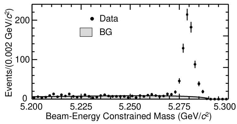
FIG. 4.: The $M_{\rm bc}$ distribution for all exclusive decay modes combined except $J/\psi K_{L}^{0}$. The $\Delta E$ cuts are imposed. The shaded area is the estimated background.

TABLE I.: Summary of $\Delta E$ signal region, the numbers of signal candidates, and expected background.

Decay	$\Delta E$ cut (MeV)	Signal	Expected
mode	Lower $\sim$ Upper	candidates	background
$B^{0}\rightarrow J/\psi K_{S}^{0}$
$~{}~{}K_{S}^{0}\rightarrow\pi^{+}\pi^{-}$	$-$40 $\sim$ 40	457	11.9
$~{}~{}K_{S}^{0}\rightarrow\pi^{0}\pi^{0}$	$-$150 $\sim$ 100	76	9.4
$B^{0}\rightarrow\psi(2S)K_{S}^{0}$
$~{}~{}\psi(2S)\rightarrow\ell^{+}\ell^{-}$	$-$40 $\sim$ 40	39	1.2
$~{}~{}\psi(2S)\rightarrow J/\psi\pi^{+}\pi^{-}$	$-$40 $\sim$ 40	46	2.1
$B^{0}\rightarrow\chi_{c1}K_{S}^{0}$	$-$40 $\sim$ 40	24	2.4
$B^{0}\rightarrow\eta_{c}K_{S}^{0}$
$~{}~{}\eta_{c}\rightarrow K_{S}^{0}K^{\pm}\pi^{\mp}$	$-$40 $\sim$ 40	23	11.3
$~{}~{}\eta_{c}\rightarrow K^{+}K^{-}\pi^{0}$	$-$60 $\sim$ 40	41	13.6
$B^{0}\rightarrow J/\psi K^{*0}$	$-$50 $\sim$ 30	41	6.7

C $B^{0}\rightarrow J/\psi K_{L}^{0}$ reconstruction

The reconstruction of $B^{0}\rightarrow J/\psi K_{L}^{0}$ is an experimental challenge but is very important because its yield is expected to be large. In addition, since this mode is a $CP$-even eigenstate, we should observe a time-dependent asymmetry reversed in sign compared to $J/\psi K_{S}^{0}$, which provides an important experimental consistency check.

While the detached vertex and invariant mass of the $K_{S}^{0}$ provide significant background reduction for $J/\psi K_{S}^{0}$, the background is larger for $J/\psi K_{L}^{0}$ as only the $K_{L}^{0}$ direction is measured. Since the energy of the $K_{L}^{0}$ is not measured, $M_{\rm bc}$ and $\Delta E$ cannot be used as the final kinematical variables to identify $B^{0}$ candidates as in other final states. Using the four-momentum of a reconstructed $J/\psi$ candidate and the $K_{L}^{0}$ flight direction, we calculate the momentum of the $K_{L}^{0}$ candidate requiring $\Delta E=0$. We then calculate $p^{\rm cms}_{B}$ which is used for the final selection.

The selection criteria are necessarily tighter than those used for the $J/\psi K_{S}^{0}$ candidates. However, precise determination of the $K_{L}^{0}$ flight direction with the KLM and ECL allows us to reconstruct $J/\psi K_{L}^{0}$ candidates with sufficient efficiency and purity.

We use tracks which are positively identified as electrons (muons) in the identification of $J/\psi\rightarrow e^{+}e^{-}~{}(\mu^{+}\mu^{-})$ candidates. We require the invariant mass of the lepton pair to lie in the range 3.05 $<M_{\ell^{+}\ell^{-}}<$ 3.13 GeV/$c^{2}$. The radiative photon correction for electron pairs is made in the same way as for the other modes. Events are rejected if one of the following decay modes are exclusively reconstructed, and satisfy $|\Delta E|<0.05$ GeV and 5.27 $<M_{\rm bc}<5.29$ GeV/$c^{2}$: $J/\psi K^{+}$, $J/\psi K_{S}^{0}$, $J/\psi K^{*+}$ $(K^{*+}\rightarrow K^{+}\pi^{0},K_{S}^{0}\pi^{+})$, and $J/\psi K^{*0}$ $(K^{*0}\rightarrow K^{+}\pi^{-},K_{S}^{0}\pi^{0})$.

We select $K_{L}^{0}$ candidates based on the KLM and ECL information. There are two classes of $K_{L}^{0}$ candidates that we refer to as KLM and ECL candidates. To select the KLM candidates, a cluster of KLM hits is formed by combining the hits within a $5^{\circ}$ opening angle. We require hits in two or more KLM layers and calculate the center of the KLM cluster. If there is an ECL cluster with energy greater than 0.16 GeV within a 15^∘ cone, we relax our criteria to allow a cluster with a hit in just one KLM layer. In this case the direction of the ECL cluster is taken as the $K_{L}^{0}$ direction. If the cluster lies within a 15^∘ cone of the extrapolation of a charged track to the first layer of the KLM, it is discarded.

ECL candidates are selected from ECL clusters using the following information: the distance between the ECL cluster and the closest charged track position; the ECL cluster energy; the ratio of energies summed in 3 $\times$ 3 and 5 $\times$ 5 arrays of CsI crystals surrounding the crystal at the center of the shower; the ECL shower width and the invariant mass of the shower. After a very loose pre-selection based on the above five discriminants, we calculate signal and background likelihood values for each discriminant based on a $J/\psi$ inclusive MC. Taking the products of the above five likelihoods for each signal and background, we form the likelihood ratio ${\cal L}_{K_{L}^{0}}/({\cal L}_{K_{L}^{0}}+{\cal L}_{\rm fake})$. This likelihood ratio is required to be greater than 0.5.

We examine the characteristics of $K_{L}^{0}$ candidates in both the data and the MC. We obtain consistent distributions for the number of $K_{L}^{0}$ candidates per event, the $K_{L}^{0}$ flight directions in the laboratory system, the total number of hit KLM layers and the number of hit first-layers in the $K_{L}^{0}$ candidates. We investigate the momentum dependence of the KLM response by using charged pions and kaons. The MC simulation reproduces the results obtained with data well. We also use $e^{+}e^{-}\to\gamma\phi$ followed by $\phi\to K_{L}^{0}K_{S}^{0}$, where the exact $K_{L}^{0}$ direction and momentum can be obtained by reconstructing $\gamma$ and $K_{S}^{0}\to\pi^{+}\pi^{-}$. These studies indicate that the $K_{L}^{0}$ identification is well reproduced by the MC with an exception of an overall detection efficiency. The $K_{L}^{0}$ detection efficiency in the data is found to be lower than the MC expectation. This, however, does not cause a difficulty in our analysis since we do not rely on the MC $K_{L}^{0}$ detection efficiency.

For both KLM and ECL candidates, we require that the $K_{L}^{0}$ direction should be within 45^∘ of its expected direction calculated from the $J/\psi$ candidate momentum assuming that the $B^{0}$ candidate was at rest in the cms. We also require that no photon from a $\pi^{0}$ decay is found near the $K_{L}^{0}$ candidate. For this requirement, we select $\pi^{0}$ candidates satisfying $0.12<M_{\gamma\gamma}<0.15$ GeV/$c^{2}$ and with momentum above 0.8 (1.2) GeV/$c$ for KLM (ECL) candidates.

To reconstruct $B^{0}\rightarrow J/\psi K_{L}^{0}$, we first use the KLM candidates. If none of the KLM candidates satisfy the selection criteria below, we use the ECL candidates. Thus, the two classes of $B^{0}\rightarrow J/\psi K_{L}^{0}$ candidates are mutually exclusive. In order to suppress the background, we calculate a probability density function (pdf) for each of the following variables and then form a product of the pdf’s to obtain the combined likelihood: the cms momentum of the $J/\psi$, $p^{\rm cms}_{J/\psi}$; the angle between the $K_{L}^{0}$ candidate and the closest charged track having a momentum larger than 0.7 GeV/$c$; the Fox-Wolfram moment ratio $R_{2}$; $\cos\theta_{B}$ where $\theta_{B}$ is the polar angle of the reconstructed $B$ in the cms; and the number of charged tracks with $p_{\rm t}>0.1$ GeV/$c$, $|dr|<$ 2 cm, and $|dz|<$ 4 cm. In addition to these five variables, two other variables are included conditionally to reduce the background from $B^{+}\rightarrow J/\psi K^{*+}$, $K^{*+}\rightarrow K_{L}^{0}\pi^{+}$ decays. One such variable is the cms momentum of the $J/\psi K_{L}^{0}\pi^{+}$ system, $p^{\rm cms}_{B}(J/\psi K_{L}^{0}\pi)$, and the other is the momentum of the additional pion. We use $p^{\rm cms}_{B}(J/\psi K_{L}^{0}\pi)$ if the invariant mass of the $K_{L}^{0}$ and a charged track, with the nominal pion mass being assumed, is above 0.85 GeV/$c^{2}$ and below 0.93 GeV/$c^{2}$, and $p^{\rm cms}_{B}(J/\psi K_{L}^{0}\pi)<0.8$ GeV/$c$[29]. The pion momentum is used if the addition of the extra pion results in $0.2<p^{\rm cms}_{B}(J/\psi K_{L}^{0}\pi)<0.45$ GeV/$c$ given the requirement above on the $K_{L}^{0}\pi^{+}$ invariant mass.

The combined likelihood is calculated for $J/\psi K_{L}^{0}$ (signal) and inclusive $B\rightarrow J/\psi$ decays (background) using MC samples. Background events from misidentified (fake) $J/\psi$ mesons are not included in the likelihood construction since their contribution is small. We then form a likelihood ratio ${\cal L}_{J/\psi K_{L}^{0}}/({\cal L}_{J/\psi K_{L}^{0}}+{\cal L}_{\rm bkg})$ that is used as a discriminant variable. Figure 5 shows the likelihood ratio distributions for the data and Monte Carlo candidates.

FIG. 5.: The likelihood ratio distributions for (a) $J/\psi K_{L}^{0}$ Monte Carlo, (b) $J/\psi$ + X background Monte Carlo, and (c) the data in the signal region with Monte Carlo events overlaid.

We require that the likelihood ratio be larger than 0.4 to identify $J/\psi K_{L}^{0}$ candidates.

Figure 6 shows the resultant $p^{\rm cms}_{B}$ distribution for events that satisfy all the selection criteria. We define the signal region as $0.2\leq p^{\rm cms}_{B}\leq 0.45~{}(0.40)~{}{\rm GeV}/c$ for $K_{L}^{0}$ candidates identified with the KLM (ECL) criteria [30], and obtain 569 candidates, out of which 397 are KLM candidates and 172 are ECL candidates.

We extract the $J/\psi K_{L}^{0}$ signal yield by fitting the $p^{\rm cms}_{B}$ distribution of the data to a sum of four components: (1) signal; (2) background with $K_{L}^{0}$; (3) background without $K_{L}^{0}$; and (4) combinatorial $J/\psi$ mesons. The shapes of the first three components are determined from the $J/\psi$ inclusive MC and look-up tables are used in the fit. The normalizations of these three components are treated as free parameters in the fit to minimize the effect of the aforementioned uncertainty in the $K^{0}_{L}$ detection efficiency in the MC simulation. The combinatorial component is evaluated using events with $e\mu$-pairs that satisfy the requirements for $J/\psi$ reconstruction. The shape is modeled by a second-order polynomial. An additional parameter of the fit is an offset in $p_{B}^{\rm cms}$, allowing the signal shape to shift with respect to the background distribution.

The result of the fit to the $p^{\rm cms}_{B}$ distribution is shown in Fig. 6. By integrating each component obtained by the fit in the signal region, we find a total of ($346.3\pm 28.8$) $J/\psi K_{L}^{0}$ signal events, and a signal purity of 61%.

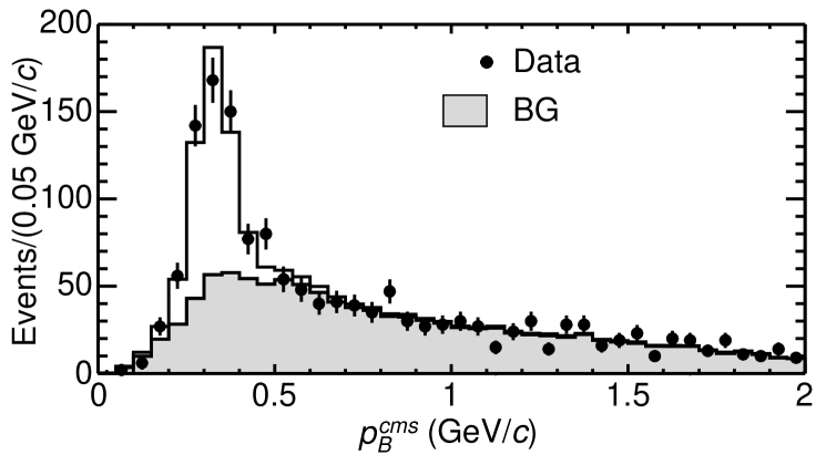
FIG. 6.: The $p_{B}^{\rm cms}$ distribution of the $J/\psi K_{L}^{0}$ candidates. The solid line is a sum of the signal and background. The shaded histogram shows the background component only.

The fitting procedure is applied to the KLM and ECL candidates separately. The $\chi^{2}$ of the fit to KLM (ECL) candidates is 54.8 (31.4) for $ndf$ = 35. Table II summarizes the fit results.

TABLE II.: Results of the fit to the $p^{\rm cms}_{B}$ distribution of the $J/\psi K_{L}^{0}$ candidates. Yields are for the signal $p^{\rm cms}_{B}$ region.

	KLM	ECL	Sum
Signal	244.8 $\pm$ 25.1	101.5 $\pm$ 14.2	346.3 $\pm$ 28.8
Background
with $K_{L}^{0}$	118.1	26.5	144.6
without $K_{L}^{0}$	27.5	38.6	66.1
Combinatorial	6.6	5.4	12.0
Total Yield	397	172	569

D Control samples of flavor-specific $B$ decays

The reconstruction of flavor-specific $B$ decays is also a key ingredient in this analysis, since such decays are used for various purposes: evaluation of the performance of flavor tagging (Section IV B); extraction of the proper-time resolution function (Section V B); $B$ lifetime measurements as a cross check (Section VI B 2); and the demonstration of null asymmetries in non-$CP$ final states (Section VI B 3). Since a large number of events with high purity are required for these purposes, we use semileptonic decays and hadronic decays from $b\rightarrow c\overline{u}d$ transitions.

For the semileptonic decays, we use the decay chains $B^{0}\to D^{*-}\ell^{+}\nu$ and $D^{*-}\to\overline{D}{}^{0}\pi^{-}$, where $\overline{D}{}^{0}\to K^{+}\pi^{-}$, $\overline{D}{}^{0}\to K^{+}\pi^{-}\pi^{0}$ and $\overline{D}{}^{0}\to K^{+}\pi^{+}\pi^{-}\pi^{-}$. All tracks used must have associated SVD hits and radial impact parameters $|dr|<0.2$ cm, except for the slow pion from the $D^{*-}$ decay. Candidate $\overline{D}{}^{0}$ decays are selected by requiring the invariant mass to be consistent with the nominal $\overline{D}{}^{0}$ mass. The invariant mass requirement depends on the $\overline{D}{}^{0}$ decay mode, varying from $+9$ to $+23~{}{\rm MeV}/c^{2}$ above the $\overline{D}{}^{0}$ mass and from $-9$ to $-37~{}{\rm MeV}/c^{2}$ below the $\overline{D}{}^{0}$ mass, respectively. For the $D^{*-}$ reconstruction, we also impose a requirement on the mass difference, $M_{\rm diff}$, between a $D^{*-}$ candidate and the corresponding $\overline{D}{}^{0}$ candidate. We require $M_{\rm diff}$ to be within $0.8$ to $1.75$ ${\rm MeV}/c^{2}$ of the nominal mass difference, depending on the $\overline{D}{}^{0}$ decay mode. In addition, we require the $D^{*-}$ cms momentum to be less than 2.6 GeV/$c$ to suppress $D^{*-}$ mesons from the continuum. The $D^{*-}$ candidates are combined with $\mu^{+}$ or $e^{+}$ candidates having the opposite charge to the $D^{*-}$ candidate. Lepton candidates must satisfy $1.4<p^{\rm cms}_{\ell}<2.4$ GeV/$c$, where $p^{\rm cms}_{\ell}$ is the cms momentum of the lepton. We exploit the massless character of the neutrino, to calculate $M_{\rm miss}^{2}$, the effective missing mass squared in the cms defined by $M_{\rm miss}^{2}\equiv(E^{\rm cms}_{B}-E^{\rm cms}_{D^{*}\ell})^{2}-|\vec{p}^{\rm~{}cms}_{B}|^{2}-|\vec{p}^{\rm~{}cms}_{D^{*}\ell}|^{2}$, and a product of the momenta of the $B$ and the $D^{*}\ell$ system, $C\equiv 2|\vec{p}^{\rm~{}cms}_{B}|\,|\vec{p}^{\rm~{}cms}_{D^{*}\ell}|$. The cosine of the angle between $\vec{p}^{\rm~{}cms}_{B}$ and $\vec{p}^{\rm~{}cms}_{D^{*}\ell}$ is given by $-M_{\rm miss}^{2}/C$. In the $M_{\rm miss}^{2}$ versus $C$ plane, therefore, we select $D^{*}\ell\nu$ candidates inside the triangle shown in Fig. 7. The triangle is defined by $C\geq-\frac{1.45}{1.595}M_{\rm miss}^{2}$, $C\geq\frac{1.02}{1.1}M_{\rm miss}^{2}$ and $C\leq-\frac{0.43}{2.695}(M_{\rm miss}^{2}+1.595)+1.45$.

FIG. 7.: The distribution of candidate $B^{0}\to D^{*-}\ell^{+}\nu$ decays in the plane of $C$ versus $M_{\rm miss}^{2}$. The signal region (triangle) is also shown.

The vertex position of the $D^{*}\ell\nu$ candidate is obtained by first fitting the vertex of the $D$ candidate from its daughter tracks, and then fitting the lepton and $D$ candidate to obtain the $B$ vertex. The slow pion track from the $D^{*}$ meson is also included in the fit. This is important since the re-fitted helix parameters of the slow pion are used to recalculate $M_{\rm diff}$ and improve its resolution. The overall signal fraction in these control samples is estimated to be 79.4%. The backgrounds consist of fake $D^{*}$ mesons (10.4%), incorrect combinations of $D^{*}$ with leptons that do not show an angular correlation (4.1%, called “uncorrelated background”), continuum events (2.1%) and $B^{\pm}$ decays (4%). The fraction of fake leptons in the uncorrelated background is estimated with a Monte Carlo simulation to be 0.5% and is neglected. We estimate the fake $D^{*}$ background by using events in the $\overline{D}{}^{0}$ mass sideband as well as fake $D^{*}$ events that are reconstructed with wrong-charge slow pions. We evaluate the uncorrelated background fraction by counting signal events in a sample wherein we flip the candidate lepton momentum vector artificially. In this case the number of uncorrelated background in the signal region remains the same level while the signal events are rejected [31]. We apply the same event selection to off-resonance data ( 2.3 fb^-1 ) and count the number of events in the signal region after subtracting the fake $D^{*}$ background. We estimate the continuum background fraction by scaling the result with the integrated luminosity. We fit the $C$ distribution with a range $-10<C<1.1$ to estimate the signal and $B\rightarrow D^{**}\ell\nu$ background fractions. We use MC information to model the signal and $B\rightarrow D^{**}\ell\nu$ distribution. The $C$ distributions and fractions of all the other backgrounds are obtained from the aforementioned special background samples and are fixed in the fit. We treat the background fraction uncertainties as a source of systematic errors in the determination of wrong tag fractions, which will be discussed in Section IV B.

For hadronic decays, we use the decay modes $B^{0}\to D^{-}\pi^{+}$, $D^{*-}\pi^{+}$ and $D^{*-}\rho^{+}$, where $D^{-}\to K^{+}\pi^{-}\pi^{-}$, $\rho^{+}\to\pi^{+}\pi^{0}$. We reconstruct $D^{*-}$ candidates in the same modes that were used for the $D^{*-}\ell^{+}\overline{\nu}$ mode. For $D$ and $D^{*-}$ candidates we apply mode-dependent requirements on the reconstructed $D$ mass (ranging from $\pm 30$ to $\pm 60$ MeV/$c^{2}$) and $M_{\rm diff}$ (ranging from $\pm 3$ to $\pm 12$ MeV/$c^{2}$), in a similar way as for $D^{*-}\ell^{+}\overline{\nu}$ mode. We select $\rho^{+}$ candidates by requiring the $\pi^{+}\pi^{0}$ invariant mass to be within 150 MeV/c² of the nominal $\rho^{+}$ mass. In order to suppress continuum background, we impose mode dependent cuts on $R_{2}$ (upper cut values ranging from 0.5 to 1.0) and $\cos\theta_{\rm thr}$ (upper cut values ranging from 0.92 to 1.0). The cut values are chosen to maximize the figure of merit $S/\sqrt{S+B}$ for each mode, where $S$ and $B$ are numbers of signal and background, respectively. We select $B^{0}$ candidates by requiring 5.27 $<M_{\rm bc}<$ 5.29 GeV/$c^{2}$ and $|\Delta E|<$ 50 MeV. Background contributions are estimated by fitting the $M_{\rm bc}$ and $\Delta E$ distributions in the same way as we do for $CP$ modes. Figure 8 shows the $M_{\rm bc}$ distribution for the three control sample modes combined. The overall signal purity is $\sim$82%. We study background components with a MC sample that includes both $B\overline{B}$ and continuum events. We find no significant peaking background in the signal region. Therefore we use the ARGUS function to model the background in the $M_{\rm bc}$ distribution. A possible deviation due to combinatorial backgrounds may introduce ambiguities in the signal fraction determination and the background $\Delta t$ model parameters of the control sample, resulting in small uncertainties in the final determination of the $CP$ asymmetry. This is considered as a source of systematic uncertainties.

FIG. 8.: $M_{\rm bc}$ distribution for all hadronic decay modes ($B^{0}\to D^{-}\pi^{+}$, $D^{*-}\pi^{+}$, and $D^{*-}\rho^{+}$) with $|\Delta E|<$ 50 MeV. Fit curves for background (dashed) and signal plus background events (solid) are superimposed.

The numbers of candidates and their purities for flavor-specific samples are summarized in Table III

TABLE III.: Summary of the numbers of flavor-specific decay candidates and their estimated purities.

Decay mode	Candidates	Purity
$B^{0}\to D^{*-}\ell^{+}\nu$	16101	79.4 %
$B^{0}\to D^{-}\pi^{+}$	2241	85.5 %
$B^{0}\to D^{*-}\pi^{+}$	2126	87.2 %
$B^{0}\to D^{*-}\rho^{+}$	1620	72.2 %

IV Flavor tagging

After the exclusive reconstruction of a neutral $B$ meson decaying into a final state, $f_{CP}$, all the remaining particles should belong to the final state, $f_{\rm tag}$, of the decay of the other $B$ meson. To observe time-dependent $CP$ violation, we need to ascertain whether $f_{\rm tag}$ is from a $B^{0}$ or ${\overline{B}{}^{0}}$. This determination is called “flavor tagging.” The simplest and most reliable method for flavor tagging uses the charge of high-momentum leptons in semileptonic decays, i.e. $B^{0}\rightarrow X\ell^{+}\nu$ and ${\overline{B}{}^{0}}\rightarrow X\ell^{-}\overline{\nu}$. The charges of final-state kaons can also be used since the decays $B^{0}\rightarrow K^{+}X$ (with $\overline{b}\rightarrow\overline{c}\rightarrow\overline{s}$) and ${\overline{B}{}^{0}}\rightarrow K^{-}X$ (with $b\rightarrow c\rightarrow s$) dominate. In addition to these two leading discriminants, our algorithm includes other categories of tracks whose charges depend on the $b$ quark’s flavor: lower momentum leptons from $c\rightarrow s\ell^{+}\nu$; $\Lambda$ baryons from the cascade decay $b\rightarrow c\rightarrow s$; high-momentum pions that originate from decays like $B^{0}\rightarrow D^{(*)-}(\pi^{+},\rho^{+},a_{1}^{+},$ etc.); and slow pions from $D^{*-}\rightarrow\overline{D}{}^{0}\pi^{-}$. All these inputs are combined, taking their correlations into account, in a way that maximizes the flavor tagging performance. The performance is characterized by two parameters, $\epsilon$ and $w$. The parameter $\epsilon$ is the raw tagging efficiency, while $w$ is the probability that the flavor tagging is wrong (wrong tag fraction). A non-zero value of $w$ results in a dilution of the true asymmetry. For example, if the true numbers of reconstructed $B^{0}$ and ${\overline{B}{}^{0}}$ are $n_{B^{0}}$ and $n_{{\overline{B}{}^{0}}}$, the corresponding asymmetry is ${\cal A}=(n_{B^{0}}-n_{{\overline{B}{}^{0}}})/(n_{B^{0}}+n_{{\overline{B}{}^{0}}})$. With realistic flavor tagging, the observed numbers are $N_{B^{0}}=\epsilon((1-w)n_{B^{0}}+wn_{{\overline{B}{}^{0}}})$ for $B^{0}$, $N_{{\overline{B}{}^{0}}}=\epsilon((1-w)n_{{\overline{B}{}^{0}}}+wn_{B^{0}})$ for ${\overline{B}{}^{0}}$, and the observed asymmetry becomes $(1-2w){\cal A}$. Since the statistical error of the measured asymmetry is proportional to $\epsilon^{-1/2}$, the number of events required to observe the asymmetry for a certain statistical significance is proportional to $\epsilon_{\rm eff}=\epsilon(1-2w)^{2}$, which is called the “effective efficiency.” Note that an imperfect knowledge of $w$ shifts the central value of the measurement and thus represents a potential source of systematic error.

In light of the above, our tagging algorithm has been designed to maximize $\epsilon_{\rm eff}$. Moreover, since $w$ directly affects the central value of our result, we have developed an approach wherein it can be determined from the data.

In our approach, we use two parameters, $q$ and $r$, to represent the tagging information. The first, $q$, corresponds to the sign of the $b$ quark charge where $q=+1$ for $\overline{b}$ and hence $B^{0}$, and $q=-1$ for $b$ and ${\overline{B}{}^{0}}$. The parameter $r$ is an event-by-event flavor-tagging dilution factor that ranges from $r=0$ for no flavor discrimination to $r=1$ for unambiguous flavor assignment. The values of $q$ and $r$ are determined for each event from a look-up table. Each entry of the table is prepared using a large statistics MC sample and is given by

$$q\cdot r\equiv\frac{N(B^{0})-N({\overline{B}{}^{0}})}{N(B^{0})+N({\overline{B}{}^{0}})},$$ (15)

where $N(B^{0})$ and $N({\overline{B}{}^{0}})$ are the numbers of $B^{0}$ and ${\overline{B}{}^{0}}$ in the MC sample.

In this analysis, we sort flavor-tagged events into six bins in $r$. For each $r$ bin, we empirically determine $w$ directly from data by using control samples, as described in Section IV B below.

A Flavor Tagging Method

Flavor tagging proceeds in two stages. In the first stage, the flavor tagging information ($q$ and $r$) provided by each track in the event is calculated. In the second, the track-level results are combined to determine event-level values for $q$ and $r$.

Tracks are sorted into four categories, namely those that resemble leptons, kaons, $\Lambda$ baryons, and slow pions. For each category, we consider several tagging discriminants, such as track momentum and particle identification information. The value of $q$ and $r$ for each track is assigned based on MC-generated look-up tables that take the tagging discriminants as input.

In the second stage, the results from the four track categories are combined to determine the values of $q$ and $r$ for each event. Again a look-up table is prepared to provide $q\cdot r$.

Figure 9 shows a schematic diagram of the flavor tagging method. The event-level parameter $r$ should satisfy $r\simeq 1-2w$ where we measure $w$ from control samples. Using this MC-determined dilution factor $r$ as a measure of the tagging quality is a straightforward and powerful way of taking into account correlations among various discriminants. Using two stages, we keep the look-up tables small enough to provide sufficient MC statistics for each entry. In the following, we provide additional details about each stage of the flavor tagging.

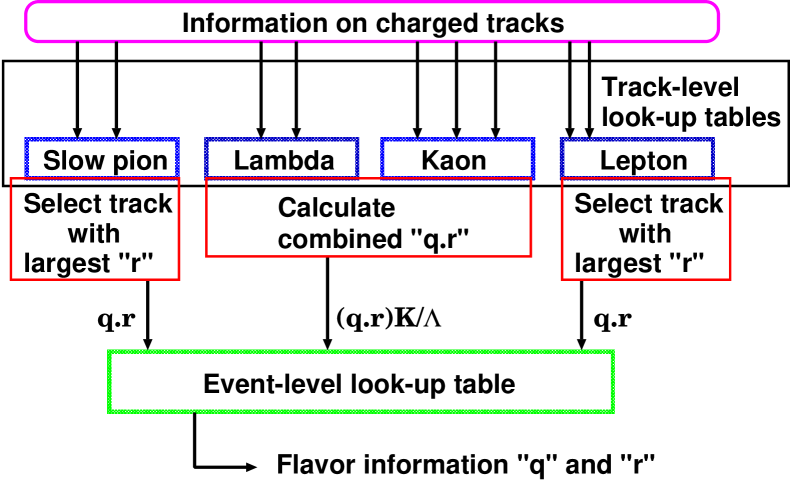
FIG. 9.: A schematic diagram of the two-stage flavor tagging. See the text on the definition of the parameters “$q$” and “$r$”.

1 Track-level flavor tagging

We select tracks that do not belong to $B_{CP}$ and that satisfy $|dr|<2$ cm and $|dz|<10$ cm. Tracks that are part of a $K_{S}^{0}$ candidate are not used. Each selected tag-side track is examined and assigned to one of the four track categories. Tracks in the lepton category are subdivided into categories for electron-like and muon-like tracks. If the cms momentum, $p^{\rm cms}_{\ell}$, of a track is larger than 0.4 GeV/$c$ and the ratio of its electron and kaon likelihoods is larger than 0.8, the track is assigned to the electron-like category. If a track has $p^{\rm cms}_{\ell}$ larger than 0.8 GeV/$c$ and the ratio of its muon and kaon likelihoods is larger than 0.95, it is passed to the muon-like category. The likelihood is calculated by combining the ACC, TOF, $dE/dx$, and ECL or KLM information. In the lepton category, leptons from semileptonic $B$ decays yield the largest effective efficiency. Leptons from $B\rightarrow D$ cascade decays and high-momentum pions from $B^{0}\rightarrow D^{(*)-}\pi^{+}X$ also make a small contribution to this category. We choose the following six discriminants: the track charge; the magnitude of the momentum in the cms, $p^{\rm cms}_{\ell}$; the polar angle in the laboratory frame, $\theta_{\rm lab}$; the recoil mass, $M_{\rm recoil}$, calculated using all the tag side tracks except the lepton candidate; the magnitude of the missing momentum in the cms, $P^{\rm cms}_{\rm miss}$; and the lepton-ID quality value.

The track charge directly provides the $b$-flavor $q$. The lepton-ID quality distinguishes leptons from pions. Its performance is reinforced by variables $p^{\rm cms}_{\ell}$ and $\theta_{\rm lab}$, which have distributions that are different for leptons and pions. The variables $p^{\rm cms}_{\ell}$, $M_{\rm recoil}$ and $P^{\rm cms}_{\rm miss}$ discriminate between high momentum leptons from semileptonic $B$ decays and intermediate momentum leptons from $B\rightarrow D$ cascade decays where the $D$ decays semi-leptonically.

If a track cannot be positively identified as a kaon and its momentum is less than 0.25 GeV/$c$, it is assigned to the slow-pion category, since low-momentum pions often come from charged $D^{*}\rightarrow D\pi$ decays. Here the discriminant variables are: the track charge; the momentum and polar angle in the laboratory frame, $p_{\rm lab}$ and $\theta_{\rm lab}$; the ratio of the electron to $\pi$ probability from $dE/dx$, and $\cos\alpha_{\rm thr}$, the cosine of the angle between the slow pion candidate and the thrust axis of the tag-side particles in the cms. The main background in this category comes from other (i.e. non-$D^{*}$ daughter) low momentum pions, electrons from photon conversions and $\pi^{0}$ Dalitz decays. To separate slow pions from those electrons we use $dE/dx$ for this class. Since the direction of the slow pion from a $D^{*}$ decay is approximately parallel to the $D^{*}$ direction, it is also almost parallel to the thrust axis. The variables $\cos\alpha_{\rm thr}$, $p_{\rm lab}$ and $\theta_{\rm lab}$, thus, help to identify the slow pions originating from $D^{*}$ decays.

If a track forms a $\Lambda$ candidate with another track, it is assigned to the $\Lambda$ category. In that category the discriminant variables are: the flavor ($\Lambda$ or $\overline{\Lambda}$); the invariant mass of the reconstructed $\Lambda$ candidate; the angle difference between the $\Lambda$ momentum vector and the direction of the $\Lambda$ vertex point from the nominal IP; the mismatch in the $z$ direction of the two tracks at the $\Lambda$ vertex point; and the proton-ID quality value.

If a track does not fall in any of the categories described above, and is not positively identified as a proton, it is classified as a kaon. The kaon category is subdivided into two parts, one for events with $K_{S}^{0}$ decays, and the other for events without $K_{S}^{0}$’s. Separate treatment is necessary as events with $K_{S}^{0}$ have a larger wrong tag fraction because of their additional strange quark content. We use the track charge, $p^{\rm cms}$, $\theta_{\rm lab}$ and the probability ratio of kaon to pion as the tagging discriminants. The charge of kaons is the most important discriminant. The other three variables help separate kaons from pions.

Although the discriminating power of high-momentum pions is weaker than that of charged kaons, they do provide some tagging information and are therefore included in the kaon category. Approximately half of the pions with $p^{\rm cms}>1.0~{}{\rm GeV}/c$ are included in the kaon category, while the other half falls into the lepton class, mostly in the muon-like category.

As is described in Section IV B, we have developed a method wherein the wrong tag fractions in our flavor tagging method are evaluated from data. Thus possible discrepancies between data and MC in the distributions of discriminant variables do not affect our $\sin 2\phi_{1}$ measurement, although they might result in the degradation in the effective efficiency. Nevertheless, we have made detailed comparisons between data and MC, which are described elsewhere [32], and obtain consistent distributions.

2 Event-level flavor tagging

The event-level flavor tagging combines the results from each of the track categories to determine an overall $q$ and $r$. For the lepton and slow-pion track categories, we take the $b$-flavor assignment from the track with the highest $r$-value in each category. For the kaon and $\Lambda$ categories, a combined $b$-flavor output is calculated as the product of likelihood values for all tracks:

$$(q\cdot r)_{K/\Lambda}=\frac{\prod_{i}[1+(q\cdot r)_{i}]-\prod_{i}[1-(q\cdot r)_{i}]}{\prod_{i}[1+(q\cdot r)_{i}]+\prod_{i}[1-(q\cdot r)_{i}]}.$$ (16)

where the subscript $i$ runs over all tracks in the kaon and $\Lambda$ categories. The product likelihood is designed to use the information from the sum of the strangeness, which provides better flavor-tagging performance than simply choosing the best candidate.

Using the three aforementioned track-level $q\cdot r$ values, the event-level $q$ and $r$ values are obtained from a look-up table that is prepared with a MC sample that is independent of the sample used to obtain $q\cdot r$ values in the track categories. The probability that we can assign a non-zero value for $r$ is 99.6% in MC; i.e. almost all the reconstructed candidates can be used to extract $\sin 2\phi_{1}$.

We specify the following six regions : $0<r\leq 0.25$, $0.25<r\leq 0.5$, $0.5<r\leq 0.625$, $0.625<r\leq 0.75$, $0.75<r\leq 0.875$ and $0.875<r\leq 1$. For each region we obtain the wrong tag fraction, $w_{l}$, where $l$ is the region ID ($l=1,...,~{}6$), using hadronic and semileptonic control samples, which is described in the next section. In this way, the analysis is insulated from systematic differences between the MC simulation and the data due to imperfections in the modeling of the detector response, decay branching fractions, and fragmentation in our MC simulation.

As a validation, we compare the distribution of $q\cdot r$ in the $D^{*}\ell\nu$ control sample with the MC expectation. As shown in Fig. 10, the data and MC are in good agreement.

FIG. 10.: The $q\cdot r$ distribution for (a) $B^{0}$ and (b) ${\overline{B}{}^{0}}$ candidates. In each figure the closed (open) points with errors show the $B^{0}\to D^{*-}\ell^{+}\nu$ (hadronic $B^{0}$ decays) data with the background subtracted, while the histogram is the MC prediction.

B Flavor Tagging Performance

The flavor tagging performance is evaluated by replacing the $CP$-eigenstate side of the event with a flavor-specific decay and tagging the $b$-flavor for the other side using the method described above. We use the semileptonic decay $B\rightarrow D^{*}\ell\nu$ and hadronic modes $B^{0}\rightarrow D^{(*)-}\pi^{+}$, and $D^{*-}\rho^{+}$ for this purpose. The overall efficiency of our flavor tagging is 99.7% which is consistent with the MC expectation.

Since we know the flavors of both $B$ mesons in this case, we can observe the time evolution of neutral $B$-meson pairs with opposite flavor (OF) or same flavor (SF), which is given by:

$${\cal P}_{\rm OF}(\Delta t) \propto 1+(1-2w)\cos(\Delta m_{d}\Delta t),$$ (17)

$${\cal P}_{\rm SF}(\Delta t) \propto 1-(1-2w)\cos(\Delta m_{d}\Delta t),$$ (18)

and the OF-SF asymmetry,

$$A_{\rm mix}\equiv{{\cal P}_{\rm OF}-{\cal P}_{\rm SF}\over{\cal P}_{\rm OF}+{\cal P}_{\rm SF}}=(1-2w)\cos(\Delta m_{d}\Delta t),$$

where $w$ is the wrong tag fraction. We thus obtain the value of $w$ directly from the data by measuring the amplitude of the OF-SF asymmetry.

We obtain the wrong tag fraction by fitting the $\Delta t$ distribution of the SF and OF events, with $\Delta m_{d}$ fixed at the world average value of 0.472 ps^-1[6]. The procedure to form the probability density function (pdf) for the fit is quite similar to that adopted for the maximum likelihood analysis of $CP$ eigenstates, which is described in the next section.

The resolution function for signal events, which models how the true distribution is smeared by the finite vertex resolution, is constructed by fitting the proper-time distributions without discriminating between the OF and SF events and with the lifetime fixed to the world average value. In the fit we use the background fraction estimated for each region of $r$, and the proper-time distribution for background obtained using events outside the signal region. For hadronic modes the sideband regions in $M_{\rm bc}$ and $\Delta E$ are used. For semileptonic decays the upper sideband in $M_{\rm diff}$ is used for the fake $D^{*}$ backgrounds. Uncorrelated backgrounds are modeled with the events that are found in the signal region after inverting the momentum of the lepton. Semileptonic decays $D^{*}X\ell\nu$ are treated as signal events since they approximately obey the same OF-SF asymmetry.

Figure 11 shows the measured OF-SF asymmetries as a function of $\Delta t$ for tagged $D^{*\mp}\ell^{\pm}\nu$ events for the six regions of $r$. The curves in the figure are obtained by the fit. The background is not subtracted in the plots.

FIG. 11.: Measured asymmetries between the OF events and the SF events (OF-SF asymmetries) for six regions of $r$ obtained for the control sample $B^{0}\rightarrow D^{*}\ell\nu$. The definition of the OF and SF events is given in the text. The background is not subtracted in the asymmetry plots. Fit curves are also shown.

For hadronic modes the fits to OF and SF events are similar to those in the semileptonic case.

We also fit signal MC samples to examine the difference between the generated and reconstructed values. We apply small corrections to $w_{l}$, that correspond to the difference. For hadronic modes the corrections range from 0.003 to 0.03 depending on the $r$ region. For semileptonic decays the difference is consistent with zero within statistical errors, and we apply no correction

To combine the results from semileptonic and hadronic decays, we calculate the weighted average and its error. We conservatively treat the difference between the weighted average and each measurement as an additional systematic error, and add this difference in quadrature with the error. The systematic errors for the semileptonic mode are dominated by the uncertainties on the background fractions and are comparable to the statistical errors. As explained in Section III D, the background estimation relies little on MC information since we use control samples whenever possible. One important exception is the $C$ distribution of the $D^{**}\ell\nu$ background; we use several $D^{**}$ components and add them with fixed fractions using MC. Since these fractions are poorly known experimentally, we conservatively assume that each component dominates the $D^{**}\ell\nu$ distribution and repeat the fit procedure to obtain the systematic error. For the hadronic modes, the main contribution to the systematic error comes from the uncertainty of the fit bias obtained from the MC simulation, but the statistical errors dominate. The event fractions and wrong tag fractions are summarized in Table IV.

TABLE IV.: The event fractions ($\epsilon_{l}$) and wrong tag fractions ($w_{l}$) for each $r$ interval. The errors include both statistical and systematic uncertainties. The event fractions are obtained from the $J/\psi K_{S}^{0}$ simulation.

$l$	$r$	$\epsilon_{l}$	$w_{l}(D^{*}\ell\nu)$	$w_{l}$(hadronic)	$w_{l}$(combined)
1	$0.000-0.250$	$0.405$	$0.463^{+0.011}_{-0.011}$	$0.469^{+0.015}_{-0.016}$	$0.465^{+0.010}_{-0.009}$
2	$0.250-0.500$	$0.149$	$0.351^{+0.019}_{-0.017}$	$0.352^{+0.026}_{-0.026}$	$0.352^{+0.015}_{-0.014}$
3	$0.500-0.625$	$0.081$	$0.254^{+0.021}_{-0.020}$	$0.219^{+0.031}_{-0.030}$	$0.243^{+0.021}_{-0.030}$
4	$0.625-0.750$	$0.099$	$0.169^{+0.019}_{-0.018}$	$0.192^{+0.028}_{-0.027}$	$0.176^{+0.022}_{-0.017}$
5	$0.750-0.875$	$0.123$	$0.107^{+0.015}_{-0.015}$	$0.127^{+0.032}_{-0.031}$	$0.110^{+0.022}_{-0.014}$
6	$0.875-1.000$	$0.140$	$0.041^{+0.012}_{-0.011}$	$0.041^{+0.024}_{-0.023}$	$0.041^{+0.011}_{-0.010}$

The total effective efficiency obtained by summing over the $r$ regions is calculated to be

$\displaystyle\epsilon_{\rm eff}=\sum_{l}\epsilon_{l}(1-2w_{l})^{2}=(27.0\pm 0.8({\rm stat})^{+0.6}_{-0.9}({\rm syst}))\%,$where $\epsilon_{l}$ is the event fraction in each of the six regions.

Our simulation indicates that events with high-momentum leptons dominate the highest $r$ region and provide the cleanest tagging information. Events with charged kaons have lower $r$, but are more numerous, and thus provide the largest contribution to the effective tagging efficiency. The effective efficiency using each category alone is examined with MC. We obtain 13% for the lepton category, 19% for the kaon and lambda categories combined, and 4% for the slow pion category. Note that the sum of these values exceeds $\epsilon_{\rm eff}$ (29.6% in MC) since an event contains tracks in different categories.

We check for possible biases in the flavor tagging by measuring the effective tagging efficiency for the $B^{0}$ and ${\overline{B}{}^{0}}$ control samples separately, and for the $q=+1$ and $-1$ samples separately. We find no statistically significant difference.

V Maximum likelihood Fit

We determine $\sin 2\phi_{1}$ by performing an unbinned maximum-likelihood fit of a $CP$ violating probability density function (pdf) to the observed $\Delta t$ distributions. These pdf’s come from the theoretical distributions diluted and smeared by the detector response. For modes other than $J/\psi K^{*0}$ the pdf expected for the signal is

$${\cal P}_{\rm sig}(\Delta t,q,w_{l},\xi_{f})=\frac{e^{-|\Delta t|/\tau_{B^{0}}}}{2\tau_{B^{0}}}{\cal P}_{CP}(\Delta t,q,w_{l},\xi_{f}),$$ (19)

where

$${\cal P}_{CP}(\Delta t,q,w_{l},\xi_{f})=1-\xi_{f}q(1-2w_{l})\sin 2\phi_{1}\sin(\Delta m_{d}\Delta t).$$ (20)

In order to take into account the effect of finite vertex resolution on the $\Delta t$ distribution, this pdf is convolved with a resolution function, $R_{\rm sig}(\Delta t)$. Our vertex reconstruction method is explained in Section V A. The parametrization and extraction of $R_{\rm sig}(\Delta t)$ are described in Section V B. We also incorporate the effect of background that dilutes the significance of $CP$ violation in the time distribution of Eq. (19). The $\Delta t$ distribution for background events, $P_{\rm bkg}(\Delta t)$, is constructed in a similar way to the signal distribution and is described in detail in Section V C.

As a result, we adopt the following $\Delta t$ distribution function for each event:

$$P(\Delta t_{i}; \sin 2\phi_{1})$$ (23)

$$=f_{\rm sig}{\displaystyle\int}{\cal P}_{\rm sig}(\Delta t^{\prime},q,w_{l},\xi_{f})R_{\rm sig}(\Delta t_{i}-\Delta t^{\prime})d\Delta t^{\prime}$$

$$+(1-f_{\rm sig})P_{\rm bkg}(\Delta t_{i}),$$

where $f_{\rm sig}$ is the probability that the event is signal, being calculated for each candidate from $p_{B}^{\rm cms}$ for $J/\psi K_{L}^{0}$ and a combination of $\Delta E$ and $M_{\rm bc}$ for other modes. The only free parameter is $\sin 2\phi_{1}$, which is determined by maximizing the likelihood function

$$L=\prod_{i}P(\Delta t_{i};\sin 2\phi_{1}),$$ (24)

where the product is over all candidates. We perform a blind analysis: The fitting algorithms were developed and finalized without using the flavor information $q$.

In the following we explain the details of $R_{\rm sig}(\Delta t)$, $P_{\rm bkg}(\Delta t)$ and $f_{\rm sig}$ in turn. The likelihood for $J/\psi K^{*0}(\rightarrow K_{S}^{0}\pi^{0})$ candidates is described separately in Section V E.

A Vertex Reconstruction

The decay vertices for the $CP$ side that include a $J/\psi$ candidate are reconstructed using leptons from the $J/\psi$ and a constraint on the $B$ decay point. The $B$ decay point is constrained by the measured profile of the interaction point (IP profile) convolved with the finite $B$ flight length in the plane perpendicular to the $z$ axis (the $r$-$\phi$ plane). The IP profile is represented by a three-dimensional Gaussian distribution. The standard deviation of each Gaussian is determined using pre-selected $B\overline{B}$ candidates on a run-by-run basis, while the mean is evaluated in finer subdivisions. The typical size of the IP profile is 100 $\mu$m in $x$, 5 $\mu$m in $y$ and 3 mm in $z$. Since the size in the $y$ direction is too small to be measured from the vertex distribution, it is taken from special measurements by the KEKB accelerator group. For leptons, we require that there are sufficient SVD hits associated with a CDC track by a Kalman filter technique; i.e. both $z$ and $r$-$\phi$ hits in at least one layer and at least one additional layer with a $z$ hit. In order to remove events with mis-reconstructed tracks, we require that the reduced $\chi^{2}$ (${\chi}^{2}/n$, $n={}$number of degrees of freedom) of the vertex be less than 20. The vertex reconstruction efficiency is measured to be 95% with $B^{\pm}\rightarrow J/\psi K^{\pm}$ and $B^{0}\rightarrow J/\psi K^{*0}(\rightarrow K^{\pm}\pi^{\mp})$ events. This is consistent with the expectation from the SVD acceptance and cluster matching efficiency. The resolution estimated by MC is typically 75$\mu$m (rms).

For $B\rightarrow\eta_{c}K_{S}^{0}$ candidates, the method is basically the same as for $J/\psi$, replacing $\ell^{+}\ell^{-}$ with $K^{+}K^{-}$ in case of $\eta_{c}\rightarrow K^{+}K^{-}\pi^{0}$ and with $K^{\pm}\pi^{\mp}$ for $\eta_{c}\rightarrow K_{S}^{0}K^{\pm}\pi^{\mp}$. Although the resolution in these cases is worse than for candidates with a $J/\psi$ vertex, it is still better than the tag-side vertex resolution.

The algorithm for tag-side vertex reconstruction is chosen to minimize the effect of long-lived particles, secondary vertices from charmed hadrons and a small fraction of poorly reconstructed tracks. From all the charged tracks except those used to reconstruct the $CP$ side, we select tracks that have associated SVD hits in the same way as for the $CP$ side. We also require that the impact parameter with respect to the $CP$-side vertex be less than 0.5 mm in the $r$-$\phi$ plane, less than 1.8 mm in $z$, and the vertex error in $z$ be less than 0.5 mm. Tracks are removed if they form a $K_{S}^{0}$ candidate satisfying $|M_{K_{S}^{0}}-M_{\pi^{+}\pi^{-}}|<15~{}{\rm MeV}/c^{2}$. Tracks satisfying these criteria are used to reconstruct the tag-side vertex where the IP constraint is also applied. If the reduced $\chi^{2}$ of the vertex is good, we accept this vertex. Otherwise we remove the track that gives the largest contribution to the $\chi^{2}$ and repeat the vertex reconstruction. If the track to be removed is a lepton with $p^{\rm cms}_{\ell}>1.1~{}{\rm GeV}/c$, however, we keep the lepton and remove the track with the second worst $\chi^{2}$. This trimming procedure is repeated until we obtain a good reduced $\chi^{2}$. The reconstruction efficiency was measured to be 93% for $B^{\pm}\rightarrow J/\psi K^{\pm}$ and $B^{0}\rightarrow J/\psi K^{*0}(\rightarrow K^{+}\pi^{-})$ candidates, consistent with the MC expectation (91%). The resolution estimated from the simulation is typically 140$\mu$m (rms).

B Signal Resolution Function

The resolution function $R_{\rm sig}(\Delta t-\Delta t^{\prime})$ is parametrized by the sum of two Gaussians:

$$R_{\rm sig}(\Delta t-\Delta t^{\prime}) = (1-f_{\rm tail})G(\Delta t-\Delta t^{\prime};\mu_{\Delta t},\sigma_{\Delta t})$$ (25)

$$+ f_{\rm tail}G(\Delta t-\Delta t^{\prime};\mu^{\rm tail}_{\Delta t},\sigma^{\rm tail}_{\Delta t}),$$ (26)

where $G(x;\mu,\sigma)$ is a Gaussian distribution in $x$ with mean $\mu$ and rms $\sigma$. The parameter $f_{\rm tail}$ describes the fraction of the tail of the resolution function, and $\sigma_{\Delta t}$, $\sigma^{\rm tail}_{\Delta t}$, $\mu_{\Delta t}$ and $\mu^{\rm tail}_{\Delta t}$ are the proper-time difference resolutions and the mean value shifts of the proper-time difference for the main part and the tail of the resolution function, respectively. The value of $f_{\rm tail}$ is determined to be $0.03\pm 0.02$ from the lifetime analysis of hadronic samples using the same resolution function.

The proper-time difference resolutions $\sigma_{\Delta t}$ and $\sigma^{\rm tail}_{\Delta t}$ are calculated on an event-by-event basis taking into account the error $\sigma_{K}$ in the kinematic approximation $\Delta t\approx\frac{\Delta z}{c\beta\gamma},\ \beta\gamma=\frac{p_{z}(\Upsilon)}{m(\Upsilon)}$:

$$\sigma_{\Delta t} = \sqrt{(\frac{\sigma_{\Delta z}}{c\beta\gamma})^{2}+\sigma_{K}^{2}},$$

$$\sigma^{\rm tail}_{\Delta t} = \sqrt{(\frac{\sigma^{\rm tail}_{\Delta z}}{c\beta\gamma})^{2}+(\sigma^{\rm tail}_{K})^{2}}.$$

We measure $\sigma_{K}=0.287\pm 0.004$ ps and $\sigma^{\rm tail}_{K}=0.32\pm 0.19$ ps using the MC simulation. These parameters are independent of the detector performance.

The parameters $\sigma_{\Delta z}$ and $\sigma^{\rm tail}_{\Delta z}$ are calculated from the event-by-event vertex errors of the two $B$ mesons, $\sigma_{z}^{CP}$ and $\sigma_{z}^{\rm tag}$, which are computed from the track helix errors in the vertex fit. We use

$$\sigma_{\Delta z}^{2} = S_{\rm det}^{2}(\sigma_{z}^{CP})^{2}+(S_{\rm det}^{2}+S_{\rm charm}^{2})(\sigma_{z}^{\rm tag})^{2},$$

$$(\sigma^{\rm tail}_{\Delta z})^{2} = (S^{\rm tail}_{\rm det})^{2}(\sigma_{z}^{CP})^{2}+\{(S^{\rm tail}_{\rm det})^{2}+(S^{\rm tail}_{\rm charm})^{2}\}(\sigma_{z}^{\rm tag})^{2},$$

where $S_{\rm charm}$ and $S^{\rm tail}_{\rm charm}$ are scaling factors to account for the degradation of the vertex resolution on the tag-side due to contamination from charm daughters, and $S_{\rm det}$ and $S^{\rm tail}_{\rm det}$ are global scaling factors that account for systematic uncertainties in the vertex errors $\sigma_{z}^{CP}$ and $\sigma_{z}^{\rm tag}$. We determine $S_{\rm charm}=0.58\pm 0.01$ and $S^{\rm tail}_{\rm charm}=2.16\pm 0.10$ using the MC simulation. The values of $S_{\rm det}$ and $S^{\rm tail}_{\rm det}$ are measured from the data as they depend on the detector performance. We determine $S_{\rm det}$ using a $D^{0}\to K^{+}\pi^{-}$ control sample. The production point of the $D^{0}$ is obtained from the primary tracks in the same hemisphere as the $D^{0}$ candidate using the IP constraint. The distance between the $D^{0}$ decay vertex and the production vertex in the $z$ direction is fit with the same resolution function and the known $D^{0}$ lifetime to obtain $S_{\rm det}$. We measure $S_{\rm det}=0.88\pm 0.01$ from the data and $S_{\rm det}=1.05\pm 0.01$ from a MC simulation of the $D^{0}$ sample. Finding $S_{\rm det}=1.035\pm 0.003$ for a $B\to J/\psi K$ MC sample, we use $S_{\rm det}=(0.88\pm 0.01)\times(1.035\pm 0.003)/(1.05\pm 0.01)=0.86\pm 0.01$ for the data. We determine $S^{\rm tail}_{\rm det}$ to be $3.51\pm 0.88$ from the lifetime analysis of the flavor-specific hadronic samples.

For $B\rightarrow\eta_{c}K_{S}^{0}$ decays, we introduce an additional scale factor to account for the difference between the $\eta_{c}$ and $J/\psi$ decays. Using the MC, we determine the additional scale factor for $\eta_{c}$ to be $1.07\pm 0.02$ for both $\eta_{c}\rightarrow K^{+}K^{-}\pi^{0}$ and $\eta_{c}\rightarrow K_{S}^{0}K^{\pm}\pi^{\mp}$.

A small fraction of events have a large reduced $\chi^{2}$. We have found that the vertex error computed from track helix errors in the vertex fit underestimates the vertex resolution and the vertex with larger $\chi^{2}$ has worse resolution. In order to take into account this effect, we introduce effective vertex resolutions $\tilde{\sigma}_{z}^{CP}$ and $\tilde{\sigma}_{z}^{\rm tag}$ when ${\chi}^{2}/n$ is greater than 3:

$$(\tilde{\sigma}_{z}^{CP})^{2} = [1+\alpha_{CP}\{({\chi}^{2}/n)_{CP}-3\}](\sigma_{z}^{CP})^{2},$$ (27)

$$(\tilde{\sigma}_{z}^{\rm tag})^{2} = [1+\alpha_{\rm tag}\{({\chi}^{2}/n)_{\rm tag}-3\}](\sigma_{z}^{\rm tag})^{2},$$ (28)

where $({\chi}^{2}/n)_{CP}$ and $({\chi}^{2}/n)_{\rm tag}$ are the reduced $\chi^{2}$ of the vertex fits for the $CP$ and tagging $B$ decay vertices, respectively. The coefficients $\alpha_{CP}=1.02\pm 0.03$ and $\alpha_{\rm tag}=1.64\pm 0.05$ are determined by a MC study of $B^{0}\rightarrow J/\psi K_{S}^{0}$.

As mentioned above, the offsets $\mu_{\Delta t}$ and $\mu^{\rm tail}_{\Delta t}$ originate from the mean shifts of the $\Delta z$ measurements $\mu_{\Delta z}$ and $\mu^{\rm tail}_{\Delta z}$, respectively:

$$\mu_{\Delta t} = \frac{\mu_{\Delta z}}{c\beta\gamma},$$

$$\mu^{\rm tail}_{\Delta t} = \frac{\mu^{\rm tail}_{\Delta z}}{c\beta\gamma}.$$

The mean value shifts, $\mu_{\Delta z}$ and $\mu^{\rm tail}_{\Delta z}$, are caused by contamination from charm daughters in the vertex reconstruction on the tag-side and are correlated with $\sigma_{z}^{\rm tag}$:

$$\mu_{\Delta z}(\sigma_{z}^{\rm tag}) = \mu_{0}+\alpha_{\mu}\sigma_{z}^{\rm tag},$$

$$\mu^{\rm tail}_{\Delta z}(\sigma_{z}^{\rm tag}) = \mu^{\rm tail}_{0}+\alpha^{\rm tail}_{\mu}\sigma_{z}^{\rm tag}.$$

The values for $\mu_{0}$ and $\mu^{\rm tail}_{0}$ are determined from hadronic samples to be $\mu_{0}=(-21.4\pm 3.7)~{}\mu$m and $\mu^{\rm tail}_{0}=(151\pm 128)$ $\mu$m, while $\alpha_{\mu}$ and $\alpha^{\rm tail}_{\mu}$ are derived from MC simulation where we obtain $\alpha_{\mu}=-0.10\pm 0.01$ and $\alpha^{\rm tail}_{\mu}=-1.42\pm 0.17$.

Figure 12 (a) shows the $\Delta t_{\rm rec}-\Delta t_{\rm gen}$ distribution for the MC $J/\psi K_{S}^{0}(\pi^{+}\pi^{-})$ candidates along with the resolution function, where $\Delta t_{\rm rec}$ and $\Delta t_{\rm gen}$ are the reconstructed and true proper-time differences, respectively. The resolution function is obtained by summing event-by-event resolution functions. The distribution is well-represented by the resolution function. The average resolution function obtained from the $J/\psi K_{S}^{0}(\pi^{+}\pi^{-})$ data is shown in Fig. 12 (b), which is represented by the sum of two Gaussian distributions with the following parameters: $\mu_{\rm main}$= $-0.24$ ps, $\mu_{\rm tail}$= 0.18 ps, $\sigma_{\rm main}$= 1.49 ps, $\sigma_{\rm tail}$= 3.85 ps.

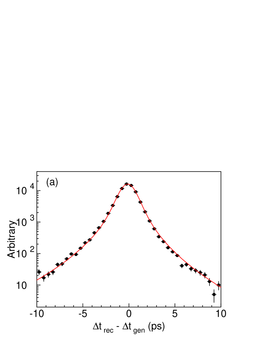
FIG. 12.: (a) The $\Delta t_{\rm rec}-\Delta t_{\rm gen}$ distributions for the MC $J/\psi K_{S}^{0}(\pi^{+}\pi^{-})$ candidates with the resolution function and (b) the average resolution function from $J/\psi K_{S}^{0}(\pi^{+}\pi^{-})$ data. The vertical scales are arbitrary.

C Background Shape

The background likelihood function is defined in a similar way to the signal function,

$$P_{\rm bkg}(\Delta t)=\int^{+\infty}_{-\infty}{\cal P}_{\rm bkg}(\Delta t^{\prime})\cdot R_{\rm bkg}(\Delta t-\Delta t^{\prime})d\Delta t^{\prime}.$$ (29)

Although $R_{\rm bkg}(\Delta t-\Delta t^{\prime})$ is treated as a resolution function for the background, it does not need to be an exact model of the vertex resolution. It is more important that $P_{\rm bkg}$ represents the proper-time distribution of the whole background sample with sufficient precision.

The pdf for background events is expressed as

$${\cal P}_{\rm bkg}(\Delta t)=f_{\tau}\frac{e^{-|\Delta t|/\tau_{\rm bkg}}}{2\tau_{\rm bkg}}+(1-f_{\tau})\delta(\Delta t^{\prime}),$$ (30)

where $f_{\tau}$ is the fraction of the background component with an effective lifetime of $\tau_{\rm bkg}$, and $\delta$ is the Dirac delta function. We assume no asymmetry in the background $\Delta t$ distribution. We find $f_{\tau}$ to be small using background-dominated regions in the $\Delta E$ versus $M_{\rm bc}$ plane of $J/\psi K_{S}^{0}$ and $J/\psi K^{+}$ candidates. We thus use ${\cal P}_{\rm bkg}(\Delta t)=\delta(\Delta t)$ for all $f_{CP}$ modes except for $J/\psi K_{L}^{0}$.

The background in the $J/\psi K_{L}^{0}$ mode is dominated by $B\to J/\psi X$ decays, including CP eigenstates that have to be treated differently from non-CP states. The ${\cal P}_{\rm bkg}$ for the $J/\psi K_{L}^{0}$ mode is determined by a MC simulation study separately for each background component: $J/\psi K^{*0}(K_{L}^{0}\pi^{0})$, $\xi_{f}=-1$ CP modes ($J/\psi K_{S}^{0}$), $\xi_{f}=+1$ CP modes ($\psi(2S)K_{L}^{0}$, $\chi_{c1}K_{L}^{0}$ and $J/\psi\pi^{0}$), the other $B^{0}$, $B^{\pm}$ decays and combinatorial background. For the CP-mode backgrounds, we use the signal pdf given in Eq. (20) with the appropriate $\xi_{f}$ values. For the $J/\psi K^{*0}(K_{L}^{0}\pi^{0})$ mode, which is a mixture of $\xi_{f}=-1$ (about $81\%$) and $\xi_{f}=+1$ (about $19\%$) states [33], we use a net CP eigenvalue of $\xi_{\psi K^{*0}}=-0.62\pm 0.11$.

Accordingly, we obtain the background pdf for $J/\psi K_{L}^{0}$

$${\cal P}_{\rm bkg} (\Delta t)\equiv\left.\frac{e^{-|\Delta t|/\tau_{B^{0}}}}{2\tau_{B^{0}}}\times\right\{f_{{\rm bg}B^{0}}$$ (35)

$$+f_{{\rm bg}\psi K^{*0}}{\cal P}_{CP}(\Delta t,q,w_{l},\xi_{\psi K^{*0}})$$

$$+f_{{\rm bg}CP_{\rm odd}}{\cal P}_{CP}(\Delta t,q,w_{l},-1)$$

$$+f_{{\rm bg}CP_{\rm even}}{\cal P}_{CP}(\Delta t,q,w_{l},+1)\left\}+f_{{\rm bg}B^{\pm}}\frac{e^{-|\Delta t|/\tau_{{\rm bg}B^{\pm}}}}{2\tau_{{\rm bg}B^{\pm}}}\right.$$

$$+f_{\rm bgCmb}\left\{f_{\tau{\rm Cmb}}\frac{e^{-|\Delta t|/\tau_{\rm bgCmb}}}{2\tau_{\rm bgCmb}}+(1-f_{\tau{\rm Cmb}})\delta(\Delta t)\right\},$$

where $f_{{\rm bg}\psi K^{*0}}$, $f_{{\rm bg}CP_{\rm odd}}$, $f_{{\rm bg}CP_{\rm even}}$, $f_{{\rm bg}B^{0}}$, $f_{{\rm bg}B^{\pm}}$, and $f_{\rm bgCmb}$ are the fractions of background components from $J/\psi K^{*0}(K_{L}^{0}\pi^{0})$, $\xi_{f}=-1$ CP-modes, $\xi_{f}=+1$ CP-modes, the remaining $B^{0}$, $B^{\pm}$, and combinatorial respectively ($f_{{\rm bg}\psi K^{*0}}+f_{{\rm bg}CP_{\rm odd}}+f_{{\rm bg}CP_{\rm even}}+f_{{\rm bg}B^{0}}+f_{{\rm bg}B^{\pm}}+f_{\rm bgCmb}=1$). The fraction of each background component is a function of $p^{\rm cms}_{B}$. The fraction, $f_{\rm bgCmb}$, is calculated as described in Section III C. The combinatorial background includes a prompt component with the fraction of $(1-f_{\tau{\rm Cmb}})$ where $f_{\tau{\rm Cmb}}$ = 0.26 $\pm$ 0.08. The lifetime distribution of the combinatorial background is obtained from $e$-$\mu$ combinations with invariant masses in the $J/\psi$ region that satisfy our selection criteria. The effective lifetime is determined to be $\tau_{\rm bgCmb}=1.03\pm 0.12$ ps, also from the $e$-$\mu$ control sample. A MC study shows that the effective lifetime for background from $B^{\pm}$, $\tau_{{\rm bg}B^{\pm}}$, is shorter than the $B^{\pm}$ lifetime due to the contamination of charged tracks from $f_{CP}$ (mostly $\pi^{\pm}$ from $J/\psi K^{*\pm}(K_{L}^{0}\pi^{\pm})$) into the tag-side vertex. The value of $\tau_{{\rm bg}B^{\pm}}$ is determined from the MC simulation to be ($1.49\pm 0.04$) ps. The same MC study shows that the effective lifetime for $B^{0}$ backgrounds is consistent with the nominal $B^{0}$ lifetime. Thus we use the nominal $B^{0}$ lifetime in our fit.

For the $J/\psi X$ background in the $J/\psi K_{L}^{0}$ mode, we use the signal resolution function $R_{\rm sig}$ to model the background since both the CP- and tag-side vertices are reconstructed with similar combinations of tracks for these backgrounds.

For the combinatorial background, we use

$$R_{\rm bkg}(\Delta t^{\prime}-\Delta t) =(1-f_{\rm tail,bkg})G(\Delta t^{\prime}-\Delta t;\mu_{\Delta t}^{\rm bkg},\sigma_{\Delta t}^{\rm bkg})$$ (37)

$$+f_{\rm tail,bkg}G(\Delta t^{\prime}-\Delta t;\mu^{\rm tail,bkg}_{\Delta t},\sigma^{\rm tail,bkg}_{\Delta t}),$$

where $f_{\rm tail,bkg}$, $\mu_{\Delta t}^{\rm bkg}$, and $\mu^{\rm tail,bkg}_{\Delta t}$ are constants determined from data. The resolutions $\sigma_{\Delta t}^{\rm bkg}$ and $\sigma^{\rm tail,bkg}_{\Delta t}$ are calculated on an event-by-event basis as

$$\sigma_{\Delta t}^{\rm bkg} = \frac{\sigma_{\Delta z}^{\rm bkg}}{c\beta\gamma},$$

$$\sigma^{\rm tail,bkg}_{\Delta t} = \frac{\sigma^{\rm tail,bkg}_{\Delta z}}{c\beta\gamma},$$

$$(\sigma_{\Delta z}^{\rm bkg})^{2} = (S_{\rm det}^{\rm bkg})^{2}[(\tilde{\sigma}_{z}^{CP})^{2}+(\tilde{\sigma}_{z}^{\rm tag})^{2}],$$

$$(\sigma^{\rm tail,bkg}_{\Delta z})^{2} = (S^{\rm tail}_{\rm bkg})^{2}[(\tilde{\sigma}_{z}^{CP})^{2}+(\tilde{\sigma}_{z}^{\rm tag})^{2}],$$

where $\tilde{\sigma}_{z}^{CP}$ and $\tilde{\sigma}_{z}^{\rm tag}$ are calculated as shown in Eq. (28).

We use different values of $\mu_{\Delta t}^{\rm bkg}$ and $\mu^{\rm tail,bkg}_{\Delta t}$ for the finite lifetime component and the zero-lifetime component, since they come from different types of events. The background shape parameters for all modes except $J/\psi K_{L}^{0}$ are obtained from events in the background-dominated regions of $\Delta E$ versus $M_{\rm bc}$. For $J/\psi K_{L}^{0}$, we use events with $e$-$\mu$ pairs to determine the properties of fake $J/\psi$ candidates, as discussed in Section III C. The parameters used in the fit are summarized in Table V.

TABLE V.: Background shape parameters for the combinatorial background.

parameters	$c\overline{c}K_{S}^{0}(K^{*0})$	$J/\psi K_{L}^{0}$
$S_{\rm det}^{\rm bkg}$	$1.08\pm 0.06$	$0.88\pm 0.07$
$S^{\rm tail}_{\rm bkg}$	$3.31\pm 0.28$	$3.94\pm 1.14$
$f_{\rm tail,bkg}$	$0.14\pm 0.04$	$0.05\pm 0.02$
lifetime component
$\mu_{\Delta t}^{\rm bkg}$(ps)	N/A	$-0.33\pm 0.10$
$\mu^{\rm tail,bkg}_{\Delta t}$(ps)	N/A	$1.86\pm 1.28$
prompt component
$\mu_{\Delta t}^{\rm bkg}$(ps)	$-0.05\pm 0.04$	$-0.22\pm 0.15$
$\mu^{\rm tail,bkg}_{\Delta t}$(ps)	$-0.12\pm 0.26$	$-5.00\pm 1.10$

D Signal probability

The signal probability, $f_{\rm sig}$, is calculated as a function of $\Delta E$ and $M_{\rm bc}$ for each event. It is given by

$$f_{\rm sig}(\Delta E,M_{\rm bc}) = \frac{F_{\rm SIG}(\Delta E,M_{\rm bc})}{F_{\rm BG}(\Delta E,M_{\rm bc})+F_{\rm SIG}(\Delta E,M_{\rm bc})},$$ (38)

where $F_{\rm SIG}(\Delta E,M_{\rm bc})$ is the signal function and $F_{\rm BG}(\Delta E,M_{\rm bc})$ is the background function.

In the case of $B^{0}\to J/\psi K_{S}$  each distribution of $\Delta E$ and $M_{\rm bc}$ is well modeled by a Gaussian function. For the background, we use a linear function for $\Delta E$ and the ARGUS parametrization[28] for $M_{\rm bc}$:

$$F_{\rm SIG} (\Delta E,M_{\rm bc})$$ (40)

$$=a\cdot G(\Delta E;\mu_{\Delta E},\sigma_{\Delta E})\cdot G(M_{\rm bc};\mu_{M_{\rm bc}},\sigma_{M_{\rm bc}}),$$

$$F_{\rm BG} (\Delta E,M_{\rm bc})$$ (43)

$$=b\cdot(1+c\cdot\Delta E)\cdot M_{\rm bc}\sqrt{1-(M_{\rm bc}/E_{\rm beam})^{2}}$$

$$\times\exp(n\cdot[1-(M_{\rm bc}/E_{\rm beam})^{2}])$$

where $a$ and $b$ are normalization factors consistent with the overall signal-to-background ratios obtained from the fit to the $M_{\rm bc}$ distribution in the $\Delta E$ signal region. The values $\sigma_{M_{\rm bc}}$, $\mu_{M_{\Delta E}}$, $\sigma_{M_{\Delta E}}$, $\mu_{M_{\rm bc}}$, $c$ and $n$ are determined from a fit to the data.

The $\Delta E$ and $M_{\rm bc}$ distributions for $B^{0}\to\psi(2S)K_{S}$($\psi(2S)\to\ell^{+}\ell^{-}$), $B^{0}\to\psi(2S)K_{S}$($\psi(2S)\to J/\psi\pi^{+}\pi^{-}$), and $B^{0}\to\eta_{c}K_{S}^{0}$ ($\eta_{c}\to K_{S}^{0}K^{\pm}\pi^{\mp}$), are determined using the same procedure as that for $B^{0}\to J/\psi K_{S}$. For $B^{0}\to\chi_{c1}K_{S}$, the $\Delta E$ and $M_{\rm bc}$ distributions are determined from MC simulation because the data sample for this mode is too small to estimate the parameters reliably.

The treatment for modes that include $\pi^{0}$ mesons such as $B^{0}\to J/\psi K_{S}$($K_{S}^{0}\to\pi^{0}\pi^{0}$) and $B^{0}\to\eta_{c}K_{S}^{0}$($\eta_{c}\to K^{+}K^{-}\pi^{0}$), is different. While the fit function for the $M_{\rm bc}$ distribution remains the same, the $\Delta E$ distributions are better represented by the Crystal Ball function[34]:

$\displaystyle\left\{\begin{array}[]{@{\,}ll}\frac{1}{\rm A}\exp(-\frac{(\Delta E-\mu_{\Delta E})^{2}}{2\sigma^{2}_{\Delta E}})&{\rm for}~{}\Delta E>\mu_{\Delta E}-\alpha\sigma_{\Delta E}\\ \frac{1}{\rm A}\frac{\exp\left({-\alpha^{2}/2}\right)}{\left[1-\frac{(\Delta E-\mu_{\Delta E})\alpha}{\sigma_{\Delta E}\alpha}-\frac{\alpha^{2}}{n}\right]^{n}}&{\rm for}~{}\Delta E<\mu_{\Delta E}-\alpha\sigma_{\Delta E}.\end{array}\right.$All the parameters for these fits were determined from MC simulation because the number of events for these modes in data is too small. The integrated background fractions in the signal region are listed in Table VI.

For the $B^{0}\rightarrow J/\psi K_{L}^{0}$ fit, we define the signal probability as a function of $p^{\rm cms}_{B}$, as described in Section III C.

TABLE VI.: Summary of the numbers of candidates and background fraction in the signal region for each mode. The values are obtained for events that have successful vertex reconstruction and flavor tagging.

Decay mode	Events	bkg. fraction
$B^{0}\rightarrow J/\psi K_{S}^{0},~{}K_{S}^{0}\rightarrow\pi^{+}\pi^{-}$	387	0.038 $\pm$ 0.010
$B^{0}\rightarrow J/\psi K_{S}^{0},~{}K_{S}^{0}\rightarrow\pi^{0}\pi^{0}$	57	0.272 $\pm$ 0.054
$B^{0}\rightarrow\psi(2S)K_{S}^{0},~{}\psi(2S)\rightarrow\ell^{+}\ell^{-}$	33	0.038 $\pm$ 0.028
$B^{0}\rightarrow\psi(2S)K_{S}^{0},~{}\psi(2S)\rightarrow J/\psi\pi^{+}\pi^{-}$	32	0.078 $\pm$ 0.027
$B^{0}\rightarrow\chi_{c1}K_{S}^{0},~{}\chi_{c1}\rightarrow J/\psi\gamma$	17	0.144 $\pm$ 0.056
$B^{0}\rightarrow\eta_{c}K_{S}^{0},~{}\eta_{c}\rightarrow K_{S}^{0}K^{\pm}\pi^{\mp}$	35	0.242 $\pm$ 0.045
$B^{0}\rightarrow\eta_{c}K_{S}^{0},~{}\eta_{c}\rightarrow K^{+}K^{-}\pi^{0}$	17	0.560 $\pm$ 0.164
$B^{0}\rightarrow J/\psi K_{L}^{0}$	523	0.379 $\pm$ 0.048
$B^{0}\rightarrow J/\psi K^{*0},~{}K^{*0}\rightarrow K_{S}^{0}\pi^{0}$	36	0.163 $\pm$ 0.054

E Likelihood for $J/\psi K^{*0}(\rightarrow K_{S}^{0}\pi^{0}$)

For the $B^{0}\rightarrow J/\psi K^{*0}$ fit, the signal pdf we use is:

$${\cal P}_{\rm sig} (\Delta t,\theta_{\rm tr},q,w_{l},\xi_{f})=\frac{e^{-|\Delta t|/\tau_{B^{0}}}}{2\tau_{B^{0}}}\times$$ (46)

$$[(1-f_{\rm odd})\frac{3}{8}(1+\cos^{2}\theta_{\rm tr}){\cal P}_{CP}(\Delta t,q,w_{l},+1)$$

$$+f_{\rm odd}\frac{3}{4}(1-\cos^{2}\theta_{\rm tr}){\cal P}_{CP}(\Delta t,q,w_{l},-1)],$$

where $f_{\rm odd}$ is the fraction of $\xi_{f}=-1$ decays in the $B^{0}\to J/\psi K^{*0}$($K^{*0}\to K_{S}^{0}\pi^{0}$) mode determined from a full angular analysis to be $0.19\pm 0.04\pm 0.04$ [33]. Here $\theta_{\rm tr}$ is defined in the transversity basis[35] as the angle between the positive $J/\psi$ decay lepton direction and the axis normal to the $K^{*0}$ decay plane in the $J/\psi$ rest frame. ${\cal P}_{CP}(\Delta t,q,w_{l},\xi_{f})$ is defined in Eq. (20). The signal resolution function is identical to that used for the other modes. For the background shape, we also use Eq. (37) for $R_{\rm bkg}$ except for the $J/\psi X$ background where we use $R_{\rm sig}$ in the same way as for the $J/\psi K_{L}^{0}$ fit.

We use the following background pdf:

$${\cal P}_{\rm bkg}(\Delta t) \equiv f_{\rm bgFA}\frac{e^{-|\Delta t|/\tau_{B_{\rm FA}}}}{2\tau_{B_{\rm FA}}}+f_{\rm bgNR}\frac{e^{-|\Delta t|/\tau_{B_{\rm NR}}}}{2\tau_{B_{\rm NR}}}$$ (47)

$$+ f_{\rm bgCmb}\delta(\Delta t),$$ (48)

where $f_{\rm bgFA}$, $f_{\rm bgNR}$, and $f_{\rm bgCmb}$ are the fractions of background components from feed-across from other $J/\psi K^{*}$ modes, non-resonant $B^{0}\to J/\psi K_{S}^{0}\pi^{0}$ decays and combinatorial background. The fractions of feed-across and non-resonant decays are determined from the MC simulation and from $K^{*}$ mass sideband events, respectively, and are functions of $M_{\rm bc}$. The fraction of combinatorial background is determined in the same way as for the $K_{S}^{0}$ modes. The effective lifetimes of the feed-across and non-resonant decay backgrounds, $\tau_{B_{\rm FA}}$ and $\tau_{B_{\rm NR}}$, are fixed to the $B^{0}$ lifetime in the fit.

Finally, the determination of $f_{\rm sig}$ follows the method for other modes that include $\pi^{0}$ mesons. The $\Delta E$ distribution is modeled by a Crystal Ball function. We consider contributions from the feed-across from other $B^{0}\to J/\psi K^{*0}$ modes as well as from the non-resonant $B^{0}\to J/\psi K_{S}^{0}\pi^{0}$ mode, which make a peak in the signal region. These background fractions are determined from the MC simulation and $K^{*0}$ mass sideband data, respectively.

VI Fit results

The likelihood fit is applied to the 1137 candidates where the vertex reconstruction and flavor tagging have been successful. We obtain

$$\sin 2\phi_{1} = 0.99\pm 0.14({\rm stat}).$$

The observed $CP$ violation is large. Figure 13 shows the $\Delta t$ distributions together with the results from the fit. Indeed, the broken $CP$ symmetry is visually apparent from the difference between the number of events for $q\xi_{f}=+1$ and $q\xi_{f}=-1$ at each $\Delta t$ bin, despite the dilution from the vertex resolution, background events and incorrect flavor tagging.

We examined the value of $\sin 2\phi_{1}$ in various sub-samples. Applying the likelihood fit to $(c\overline{c})K_{S}^{0}~{}(\xi_{f}=-1)$ and $J/\psi K_{L}^{0}~{}(\xi_{f}=+1)$ separately, we obtain $\sin 2\phi_{1}=0.84\pm 0.17({\rm stat})$ and $1.31\pm 0.23({\rm stat})$, respectively. Figure 14 shows the log-likelihood values as a function of $\sin 2\phi_{1}$ for $CP$-odd, $CP$-even, and all decay modes. A more detailed breakdown along with separate results for $q=+1$ and $-1$ is given in Table VII. We find no systematic trends beyond statistical fluctuations.

TABLE VII.: Summary of $\sin 2\phi_{1}$ fit results. Only statistical errors are shown.

Sample	Events	$\sin 2\phi_{1}$
$f_{\rm tag}=B^{0}$ ($q=+1$)	560	$0.84\pm 0.21$
$f_{\rm tag}=\overline{B}{}^{0}$ ($q=-1$)	577	$1.11\pm 0.17$
$(c\overline{c})K_{S}^{0}$	578	$0.84\pm 0.17$
$J/\psi K_{S}^{0}(\pi^{+}\pi^{-})$	387	$0.81\pm 0.20$
$(c\overline{c})K_{S}^{0}$ except $J/\psi K_{S}^{0}(\pi^{+}\pi^{-})$	191	$1.00\pm 0.40$
$J/\psi K_{L}^{0}$	523	$1.31\pm 0.23$
$J/\psi K^{*0}(K_{S}^{0}\pi^{0})$[36]	36	$0.97\pm 1.40$
All	1137	$0.99\pm 0.14$

Figure 15 shows the asymmetry, $\sin 2\phi_{1}\cdot\sin(\Delta m_{d}\Delta t)$, obtained in each $\Delta t$ bin for (a) all modes, (b) $CP$-odd modes and (c) $CP$-even modes. The unbinned maximum likelihood fit is performed separately for events in each $\Delta t$ bin. The value of $\sin 2\phi_{1}$ and its error are multiplied by the average value of $\sin(\Delta m_{d}\Delta t)$ in each $\Delta t$ bin of the plot. The points are plotted at the average $\Delta t$ of each bin.

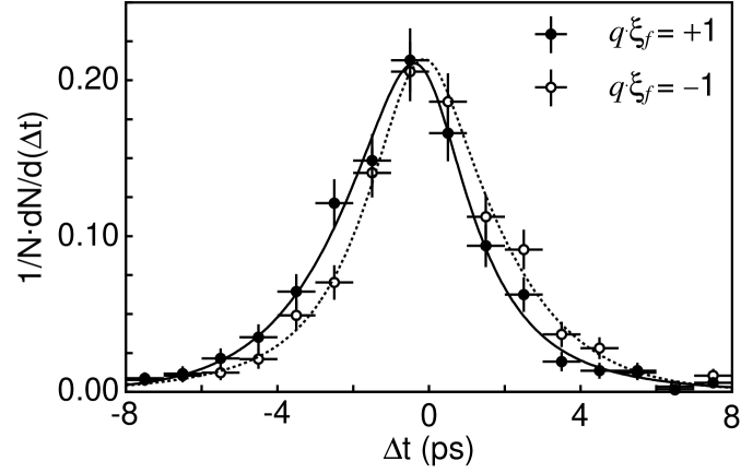
FIG. 13.: $\Delta t$ distributions for the events with $q\xi_{f}=+1$ (solid points) and $q\xi_{f}=-1$ (open points). The results of the global fit (with $\sin 2\phi_{1}=0.99$) are shown as solid and dashed curves, respectively.

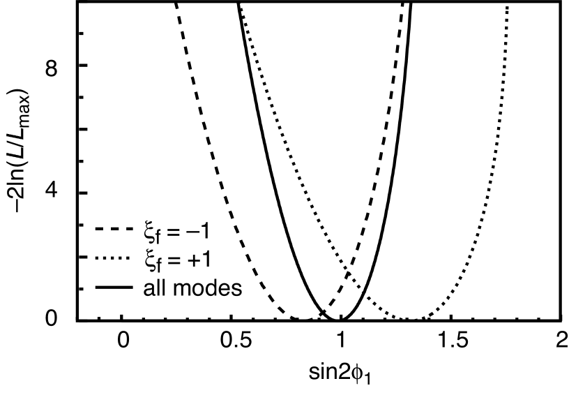
FIG. 14.: Values of $-2\ln(L/L_{\rm max})$ vs. $\sin 2\phi_{1}$ for the $\xi_{f}=-1$(dashed) and $+1$(dotted) modes separately and for both modes combined(solid).

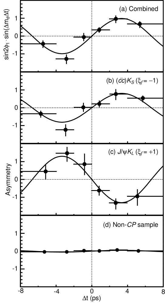
FIG. 15.: (a) The asymmetry obtained from separate fits to each $\Delta t$ bin for the full data sample; the curve is the result of the global fit. The corresponding plots for the (b) $(c\overline{c})K_{S}^{0}$ ($\xi_{f}=-1$), (c) $J/\psi K_{L}^{0}$ ($\xi_{f}=+1$) and (d) non-CP $B^{0}$ control samples are also shown. The curves are the results of the combined fit applied separately to the individual data samples.

We also checked the values of $\sin 2\phi_{1}$ in the different $r$ ranges of the flavor tagging. The results are listed in Table VIII. No systematic variation is seen. Finally, we subdivided the $CP$ sample into three data taking periods: in 2000, from January to April 2001 and the rest. The $\sin 2\phi_{1}$ values we obtain are $0.84\pm 0.29$(stat), $1.33\pm 0.30$(stat) and $0.94\pm 0.20$(stat), respectively. Again the results are consistent within the statistical fluctuations.

TABLE VIII.: The $r$ dependence of $\sin 2\phi_{1}$ fit result. Only statistical errors are shown.

$r$ region	0.0-0.5	0.5-0.75	0.75-0.875	0.875-1.0
Events	613	239	119	166
$\sin 2\phi_{1}$	$0.60^{~{}+0.65}_{~{}-0.67}$	$0.40^{~{}+0.31}_{~{}-0.32}$	$1.56^{~{}+0.25}_{~{}-0.29}$	$1.05^{~{}+0.15}_{~{}-0.18}$

A Systematic Errors

The sources of systematic error we consider are listed in Table IX[37]. Adding all the systematic errors in quadrature, we obtain

$$\sin 2\phi_{1}=0.99\pm 0.14({\rm stat})\pm 0.06({\rm syst}).$$

TABLE IX.: List of systematic errors on $\sin 2\phi_{1}$.

source	$+$error	$-$error
vertex reconstruction	+0.040	$-$0.040
resolution function	+0.022	$-$0.032
wrong tag fraction	+0.022	$-$0.025
physics ($\tau_{B^{0}}$, $\Delta m_{d}$, $J/\psi K^{*0}$)	+0.007	$-$0.004
background fraction (except for $J/\psi K_{L}^{0}$)	+0.003	$-$0.004
background fraction ($J/\psi K_{L}^{0}$)	+0.020	$-$0.020
background shape	+0.001	$-$0.001
total	+0.06	$-$0.06

Below we explain each item in order.

1 Vertex reconstruction

The largest contribution comes from vertex reconstruction. We searched for possible biases by using two different vertexing algorithms and changing the track selection criteria for the tag-side vertex. In the alternative vertexing algorithm, we first obtain a seed vertex using tracks of good quality: an impact parameter from IP in $r$-$\phi$ direction is smaller than 2.5 times the $r$-$\phi$ vertex error; the vertex error in $z$ is less than 0.5 mm; and the cms momenta are larger than 0.3 GeV/$c$. We then repeat the vertex fit using tracks within 3 (4) $\sigma$ in $z$ from the seed vertex for the cms track momentum less (larger) than 1 GeV/$c$, where $\sigma$ is the error of the seed vertex in $z$. We also estimated the effects of the vertex resolution tails using samples with small $\Delta t$ ($|\Delta t|<6$ ps) and tighter vertex quality cuts.

2 Resolution function

We estimate the contribution due to the uncertainty in the resolution function by varying its parameters (given in Section V B) by $\pm 1\sigma$.

3 Wrong tag fraction

Systematic errors due to uncertainties in the wrong tag fractions given in Section IV B (Table IV) are studied by varying wrong tag fraction individually for each $r$ region. We added the contributions from each variation in quadrature.

4 Physics parameters

The $B$ meson lifetime and mixing parameter are fixed to the world average values[6] in our fit; i.e. $\tau_{B}=(1.548\pm 0.032)$ ps and $\Delta m_{d}=(0.472\pm 0.017)$ ps^-1. We estimate the systematic error by repeating the fit varying these parameters by their errors. Another physics-related uncertainty is the $CP$ eigenvalue of $J/\psi K^{*0}$ ($\xi_{J/\psi K^{*0}}$) measured from the angular distribution of the decay daughters[33]. This systematic uncertainty is determined from the $\pm 1\sigma$ uncertainty in the measurement.

5 Background fraction except for $J/\psi K_{L}^{0}$

The background fraction in our pdf, $1-f_{\rm sig}$, is calculated from the signal and background distribution functions of $\Delta E$ and $M_{\rm bc}$ as described in Section  V D. The distribution functions of $\Delta E$ and $M_{\rm bc}$ are determined from data or the MC simulation depending on the decay mode. To estimate the systematic errors associated with the choice of parameterization, we varied the parameters obtained from the MC simulation by $\pm 2\sigma$ and the parameters obtained from the data by $\pm 1\sigma$. The likelihood fit was repeated. A wider range of uncertainty was conservatively chosen for parameters obtained from the MC simulation to take into account the possible difference between the MC simulation and data. We also estimated the systematic errors for the integrated background fractions, listed in Table VI, by varying these parameters by $\pm 1\sigma$. We added the results of these calculations for each decay mode in quadrature.

6 Background fraction for $J/\psi K_{L}^{0}$

As described in Section III C, the background fraction for the $J/\psi K_{L}^{0}$ sample is obtained from a fit to $p^{\rm cms}_{B}$ distribution and is given in Table II. In this fit, the sum of components is automatically constrained to the total number of events in the signal region. Thus, the signal yield and the size of other backgrounds are strongly anti-correlated. To determine the systematic error on $\sin 2\phi_{1}$ that comes from the uncertainty of the background, we need to take this anti-correlation into account. To this end, we repeat the fit to the $p^{\rm cms}_{B}$ distribution with the background fractions as free parameters but with the signal yield fixed +1$\sigma$ or $-$1$\sigma$ away from the central value obtained in the nominal fit. The resultant background yields are used to repeat the procedure to obtain $\sin 2\phi_{1}$. We regard the difference between the thus obtained value and our nominal $\sin 2\phi_{1}$ value as the systematic error. We also check the systematic error due to the uncertainty in the CP content of the background. We repeated the fit varying parameters to determine the various background fractions. Since these parameters are obtained from the MC simulation, we estimate the systematic error by conservatively changing each parameter by $\pm 2\sigma$ and adding the resulting changes in quadrature.

7 Background shape

The parameters that determine ${\cal P}_{\rm bkg}(\Delta t)$ and $R_{\rm bkg}$, given in Section V C, are varied within their errors and fits are repeated.

B Cross checks

We performed several cross checks: The fitting procedure was examined using MC samples based on our likelihood functions (toy MC samples). We also measured the $B$ meson lifetime using the same vertex reconstruction method. In addition we tested non-$CP$ control samples. These cross checks are described below.

1 Ensemble test

A thousand toy MC samples, each containing 1137 events, are generated based on our likelihood function to check the fitting procedure. Figure 16 shows the distribution of residuals ($\sin 2\phi_{1}$(fit) $-\sin 2\phi_{1}$(input)), pulls (residuals divided by fit errors), and the positive and negative errors on $\sin 2\phi_{1}$ returned from the fits. All the toy MC samples have an input value of $\sin 2\phi_{1}=0.99$. The center of the residual in Fig. 16 (a) is consistent with zero, and the standard deviation of the pull distribution in Fig. 16 (b) is consistent with unity. Therefore the global fit returns the input $\sin 2\phi_{1}$ value and a reasonable error. Figure 16 (c) and (d) also show that the positive and negative errors obtained from the fit are consistent with expectations.

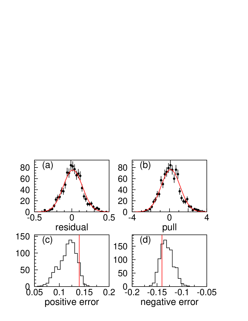
FIG. 16.: The result of our toy Monte Carlo test of our fit: (a) the distribution of residuals ( $\sin 2\phi_{1}$(fit) $-\sin 2\phi_{1}$(input) ), (b) pull distribution ( (residual)/(error of fit) ), and (c) the positive and (d) negative errors of $\sin 2\phi_{1}$ returned from the fits. The vertical lines in figures (c) and (d) indicate the errors obtained from the fit to data.

We also generate toy MC samples for $J/\psi K^{0}_{S}$ and $J/\psi K^{0}_{L}$. The average negative errors are 0.19 and 0.28 for $J/\psi K^{0}_{S}$ and $J/\psi K^{0}_{L}$, respectively. Our measurement for $J/\psi K^{0}_{S}$ (0.20) is in good agreement with the expectation, while the result for for $J/\psi K^{0}_{L}$ (0.23) is smaller. We obtain the probability of obtaining smaller errors than this measurement to be 1.4% for $J/\psi K^{0}_{L}$, which is within a possible fluctuation.

2 $B^{0}$ lifetime

The $B^{0}$ lifetime has been measured with the same data sample. We apply the same vertex reconstruction algorithm for fully reconstructed $B^{0}$ decays as for the $CP$ decays and the tracks on the tag-side. Unbinned maximum likelihood fits are made with an exponential pdf convolved with the same $\Delta t$ resolution function and background pdf as in the fit for $CP$ eigenstates. For the combined $B^{0}\to J/\psi K^{*0}(K^{+}\pi^{-})$, $D^{(*)-}\pi^{+}$, $D^{*-}\rho^{+}$ and $D^{*-}\ell^{+}\nu$ decay modes, the $B^{0}$ lifetime is measured to be $\tau_{B^{0}}=1.547\pm 0.021({\rm stat.})$ ps. The result is consistent with the world average value[6].

3 Tests on control samples

We use control samples of non-$CP$ eigenstates, $B^{0}\rightarrow J/\psi K^{*}(K^{+}\pi^{-})$, $B^{0}\rightarrow D^{(*)-}\pi^{+}$, $B^{0}\rightarrow D^{*-}\rho^{+}$ and $B^{0}\rightarrow D^{*-}\ell^{+}\nu$, to check for biases in the analysis. We perform the same fit to these control samples as for the $CP$-eigenstate modes. The results, summarized in Table X, show no systematic tendency. A combined fit to all the modes yields $0.05\pm 0.04$, consistent with zero at the $1.2\sigma$ level, as shown in Fig. 15 (d).

TABLE X.: $CP$ asymmetries for control samples.

	$J/\psi K^{*0}(K^{+}\pi^{-})$	$D^{(*)-}\pi^{+}$	$D^{*-}\ell^{+}\nu$
		and $D^{*-}\rho^{+}$
Events	816	5560	10232
$CP$ asymmetry	$0.01\pm 0.14$	$0.12\pm 0.06$	$0.01\pm 0.05$

We check for a possible bias due to $CP$ asymmetry in the background. We fit $J/\psi K_{L}^{0}$ candidates in the background region (1.0 $<p^{\rm cms}_{B}<$ 2.0 GeV/$c$) treating all the events as $J/\psi K_{L}^{0}$ candidates. Note that the fraction of events with definite $CP$ in this region of $p^{\rm cms}_{B}$ is expected to be negligible. The result is $\sin 2\phi_{1}=0.49~{}\pm 0.35$, consistent with zero at the 1.4$\sigma$ level.

C Discussion

We have performed several statistical analyses of the results described in the previous sections. Using a Gaussian likelihood function based on the statistical and the systematic errors, we calculated the confidence intervals bounded by the physical region for $\sin 2\phi_{1}$ using two methods: the Feldman-Cousins[38] frequentist approach and the Bayesian method with a flat prior pdf. We find a lower bound on $\sin 2\phi_{1}$ of 0.70 at the 95% C.L. in both cases. We also estimated the Bayesian lower limit using the exact likelihood function, shown in Fig. 14, and obtained 0.69. We conclude that the likelihood function is Gaussian to a good approximation. Combinations of indirect measurements typically constrain $0.50<\sin 2\phi_{1}<0.86$ in the framework of the SM[39]. Although our measured value is large, it is consistent with the higher range of the SM prediction. We are continuing the measurement with much higher statistics in order to test the KM ansatz more precisely.

Finally we comment on the possibility of direct $CP$ violation. The signal pdf for a neutral $B$ meson decaying into a $CP$ eigenstate (Eqs. 19 and 20) can be expressed in a more general form as

$${\cal P}_{\rm sig} (\Delta t,q,w_{l},\xi_{f})=\frac{e^{-|\Delta t|/\tau_{B^{0}}}}{2\tau_{B^{0}}(1+|\lambda|^{2})}\times$$ (51)

$$\left\{{1+|\lambda|^{2}\over 2}-q(1-2w_{l})[\xi_{f}{\cal A}|\lambda|\sin(\Delta m_{d}\Delta t)\right.$$

$$\left.-{|\lambda|^{2}-1\over 2}\cos(\Delta m_{d}\Delta t)]\right\},$$

where $\lambda$ is a complex parameter that depends on both $B^{0}{\overline{B}{}^{0}}$ mixing and on the amplitudes for $B^{0}$ and ${\overline{B}{}^{0}}$ decay to a $CP$ eigenstate[2]. The coefficient of $\sin(\Delta m_{d}\Delta t)$ is given by ${\cal A}|\lambda|=-\xi_{f}Im\lambda$ and is equal to $\sin 2\phi_{1}$ in the SM. The presence of the cosine term ($|\lambda|\neq 1$) would indicate direct $CP$ violation. Throughout our study we have assumed $|\lambda|=1$, as expected in the SM[2]. In order to test this assumption, we also performed a fit using the above expression with ${\cal A}$ and $|\lambda|$ as free parameters, keeping everything else the same. We obtain $|\lambda|=1.09\pm 0.14$ and ${\cal A}=0.80\pm 0.19$ for the $J/\psi K_{S}^{0}(\pi^{+}\pi^{-})$ sample only, and $|\lambda|=1.03\pm 0.09$ and ${\cal A}=0.99\pm 0.14$ for all $CP$ modes combined, where the errors are statistical only. This result confirms the assumption used in our analysis.

VII Conclusion

We have measured the $CP$ violation parameter $\sin 2\phi_{1}$ at the KEKB asymmetric $e^{+}e^{-}$ collider using a data sample of 29.1 fb^-1 recorded on the $\Upsilon(4S)$ resonance with the Belle detector. To extract $\sin 2\phi_{1}$, we apply a maximum likelihood fit to the 1137 candidate $B$ meson decays to $CP$ eigenstates. We obtain

$\displaystyle\sin 2\phi_{1}=0.99\pm 0.14({\rm stat})\pm 0.06({\rm syst}).$We conclude that there is large $CP$ violation in the neutral $B$ meson system. A zero value for $\sin 2\phi_{1}$ is ruled out by more than six standard deviations.

We have calculated the confidence intervals bounded by the $\sin 2\phi_{1}$ physical region for the Bayesian and Feldman-Cousins frequentist approaches. The lower bound is found to be 0.70 at the 95% C.L. in both cases. Our result is consistent with the higher range of values allowed from the constraints of the Standard Model as well as with our previous measurements[9].