THE BNL MUON ANOMALOUS MAGNETIC MOMENT MEASUREMENT

The E821 experiment at Brookhaven National Laboratory is designed to measure the muon magnetic anomaly, $a_{\mu}$, to an ultimate precision of 0.4 parts per million (ppm). Because theory can predict $a_{\mu}$ to 0.6 ppm, and ongoing efforts aim to reduce this uncertainty, the comparison represents an important and sensitive test of new physics. At the time of this Workshop, the reported experimental result from the 1999 running period achieved $a_{\mu^{+}}~{}=11\,659\,202(14)(6)\times 10^{-10}$ (1.3 ppm) and differed from the most precise theory evaluation by 2.6 standard deviations. Considerable additional data has already been obtained in 2000 and 2001 and the analysis of this data is proceeding well. Intense theoretical activity has also taken place ranging from suggestions of the new physics which could account for the deviation to careful re-examination of the standard model contributions themselves. Recently, a re-evaluation of the pion pole contribution to the hadronic light-by-light process exposed a sign error in earlier studies used in the standard theory. With this correction incorporated, experiment and theory disagree by a modest 1.6 standard deviations.

1 Introduction

A precision measurement of the muon anomalous magnetic moment, $a_{\mu}~{}=(g-2)/2$, is a sensitive test of physics beyond the standard model. Because contributions to the muon anomaly from known processes (see Fig. 1), such as QED, the weak interaction, and hadronic vacuum polarization (including higher-order terms) are believed to be understood at the sub-ppm level, any significant difference between experiment and theory suggests a yet unknown, and thus not included, physical process. $\!{}^{{\bf?}}$ Conversely, agreement between theory and experiment can set tight constraints on new physics. Many standard model extensions have been postulated; of these, quite a few would manifest themselves in additional contributions to $a_{\mu}$ at the ppm level. This indirect method of probing high-mass and short-distance physics is being used by the Brookhaven E821 Collaboration $\!{}^{{\bf?}}$ in a new measurement $\!{}^{{\bf?},{\bf?},{\bf?}}$ of $a_{\mu}$. The experimental work is complemented by an aggressive effort by others to improve the precision of the standard model theory. In the near-term future, and generally in advance of the direct-discovery possibilities at the Tevatron or the LHC, both experiment and theory should achieve relative precision near or below 0.5 ppm.

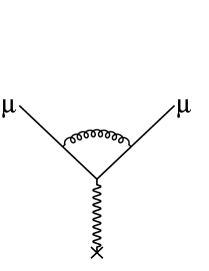
(a) QED

(b) Weak

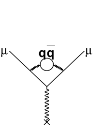
(c) Hadronic

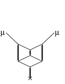
(d) Light-by-light

Figure 1: Representative first-order Feynman diagrams for QED, weak and hadronic vacuum polarization, and hadronic light-by-light scattering.

The Collaboration recently reported $\!{}^{{\bf?}}$ a 1.3 ppm precision measurement of $a_{\mu}$ based on data obtained in the 1999 running period. A summary $\!{}^{{\bf?}}$ of the most up-to-date theoretical information implied a deviation from theory by $2.6\sigma$. Subsequently, re-examinations of the 1st-order hadronic vacuum polarization (HVP) contribution suggested some scatter in the central theory value, however the deviation remained greater than two standard deviations. Shortly after this Workshop, Knecht and Nyffeler reported $\!{}^{{\bf?}}$ a new calculation of the hadronic light-by-light (LbL) diagram (see Fig. 1d). This process cannot be determined from measurements and therefore must be estimated using theoretical models. It has endured a checkered past in which the sign was once reversed from positive to negative. The new finding finds a positive sign for the dominant pion pole contribution, but otherwise a similar magnitude to previous studies by others. $\!{}^{{\bf?},{\bf?}}$ This finding prompted Hayakawa and Kinoshita to reexamine their own work $\!{}^{{\bf?}}$ which indeed contained a sign error—in an innocent computer algorithm—prompting a report $\!{}^{{\bf?}}$ with a new hadronic light-by-light term of $a_{\mu}(\rm{LbL})=+89.6(15.4)\times 10^{-11}$. Combined with the other complete hadronic LbL evaluation by Bijnens et al.,$\!{}^{{\bf?}}$ which has also been updated to report $\!{}^{{\bf?}}$ a sign error, the standard model summary $\!{}^{{\bf?}}$ is $a_{\mu}$(thy) $=11~{}659~{}176.7(6.7)\times 10^{-10}$. This adjustment reduces $\Delta a_{\mu}(\rm{exp-thy})$ by $\approx 1$ standard deviation and puts the discrepancy with the standard model at the modest $1.6\sigma$ level.

This Workshop also featured two talks by leading contributors to the 1st-order HVP evaluation. Simon Eidelman $\!{}^{{\bf?}}$ described the recent data obtained by the Novosibirsk CMD-II team in their experiment on $e^{+}e^{-}\rightarrow$ Hadrons in the important $\rho$ region. These data alone, when finalized, should reduce the uncertainty to the 0.6 ppm level without the inclusion of hadronic tau decays. Andreas Höcker,$\!{}^{{\bf?}}$ together with Michel Davier, pioneered the inclusion of hadronic tau decay data in the evaluation of the HVP term. Despite non-negligible isospin breaking considerations, their results were responsible for a significant decrease in the overall SM theory uncertainty. But their work is not without some controversy and questioning.$\!{}^{{\bf?}}$ Additional tau data have been analyzed and the present issue discussed at this Workshop was the reliability with respect to the more direct $e^{+}e^{-}$ approach; the question raised was, “Can the tau data be used with sub-percent level absolute precision?” The answer is still unclear. On the horizon experimentally is the use of radiative return at higher-energy $e^{+}e^{-}$ machines which promises to add complementary precision input to the HVP database. As one has witnessed over the past year, the standard model theory of $a_{\mu}$ is very much a work in progress, just like the experiment.

Recent 1st-order HVP evaluations are shown in Fig. 2. They are compared to the new E821 result and the current world average. The QED, weak and higher-order hadronic terms, which are believed to be known to a few tenths of a ppm or better, have been subtracted from the measurement of $a_{\mu}$. This results in an effective “experiment-to-experiment” comparison because the input to the 1st-order HVP comes from measurement. The plot demonstrates the present relative size of the uncertainties. Both experiment and “theory” uncertainties will be reduced with the analysis of additional data already obtained.

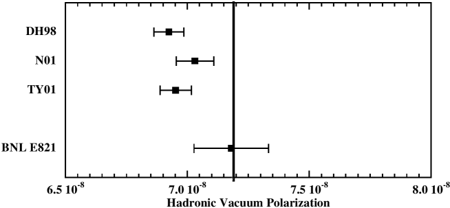
Figure 2: Recent 1st-order HVP evaluations by Davier and Höcker,$\!{}^{{\bf?}}$ Narison $\!{}^{{\bf?}}$ and de Trocóniz and Ynduráin,$\!{}^{{\bf?}}$ each combining $e^{+}e^{-}$ and hadronic tau decay data. The 1999 BNL result is shown with the QED, weak and higher-order hadronic terms subtracted. The solid vertical line represents the current world average experimental result.

Bill Marciano $\!{}^{{\bf?}}$ speculated on the implications of the comparison of final data with settled theory. A non-standard model result could be explained rather naturally in the context of supersymmetry. It has been recognized for some years that the muon anomaly scales nearly linearly with $\tan\beta$, the ratio of Higgs doublet vacuum expectation values in the theory. The SUSY allowed phase space certainly has ample room for large $\tan\beta$ solutions, while the lowest values, which would be exceedingly difficult to observe in $a_{\mu}$ are beginning to be ruled out by direct search experiments. Of course, many other candidate explanations for non-SM $a_{\mu}$ exist; many $\!{}^{{\bf?}}$ have been published following the original $2.6\sigma$ deviation report.

The purpose of this paper is to describe the new experiment which was designed following the three pioneering CERN efforts. Francis Farley $\!{}^{{\bf?}}$ presented the historical development and the key ideas incorporated in all $(g-2)$ experiments. I will concentrate here on the specifics related to the E821 implementation and the 1999 data analysis.

2 The E821 Experiment

2.1 Principle

The experimental goal is to measure directly $(g-2)$  and not $g$. The leading-order contribution to $a_{\mu}=(g-2)/2$ is the QED “Schwinger” term whose magnitude is $(\alpha/2\pi)\approx 1.16\times 10^{-3}$. This implies that to measure $g$ directly to an equivalent sensitivity would require an experiment with nearly an 800-fold increase in precision.

The muon anomaly is determined from the difference between the cyclotron and spin precession frequencies for muons contained in a magnetic storage ring, namely

$$\vec{\omega}_{a}=-{e\over m}\left[a_{\mu}\vec{B}-\left(a_{\mu}-{1\over\gamma^{2}-1}\right)\vec{\beta}\times\vec{E}\right].$$ (1)

In principle, an additional $\vec{\beta}\cdot\vec{B}$ term exists. However, it vanishes when the muon trajectory is perpendicular to the magnetic field as is the case in this experiment. Because electric quadrupoles are used to provide vertical focussing in the storage ring, the $\vec{\beta}\times\vec{E}$ term is necessary and illustrates the sensitivity of the spin motion to a static electric field. This term conveniently vanishes for the “magic” momentum of 3.094 GeV/$c$ where $\gamma=29.3$. The experiment is therefore built around the principle of production and storage of muons centered at this momentum in order to minimize the electric field effect. Because of the finite momentum spread of the stored muons, a modest correction to the observed precession frequency is made to account for the muons above or below the magic momentum. Vertical betatron oscillations induced by the electric field imply that the plane of the muon precession has a time-dependent pitch. Accounting for both of these electric-field related effects introduces a $+0.81\pm 0.08$ ppm correction to the measured precession frequency.

Muons introduced into the storage ring exhibit cyclotron motion and their spins precess until the time of decay; $\gamma\tau_{\mu}\approx 64.4~{}\mu s$. The net spin precession depends on the integrated path followed by a muon convoluted with the local magnetic field experienced along the path.

Parity violation leads to a preference for the highest-energy decay electrons to be emitted in the direction of the muon spin. Therefore, a snapshot of the muon spin direction at time $t$ after injection into the storage ring is obtained, again on average, by the selection of decay electrons in the upper part of the Lorentz-boosted Michel spectrum ($E_{max}\approx 3.1$ GeV). The number of electrons above a selected energy threshold is modulated at frequency $\omega_{a}$ with a threshold-dependent asymmetry $A=A(E_{th})$. The decay electron distribution is described by

$$N(t)=N_{0}\exp(-t/\gamma\tau_{\mu})\left[1+A\cos(\mbox{$\omega_{a}$}t+\phi)\right],$$ (2)

where $N_{0}$, the normalization, $A$ and $\phi$ are all dependent on the energy threshold $E_{th}$. For $E_{th}=2.0$ GeV, $A\approx 0.4$.

In summary, the experiment involves the measurement of three quantities: (1) The precession frequency, $\omega_{a}$ in Eq. 1; (2) The muon distribution in the storage ring; and, (3) The time-averaged local magnetic field. The muon anomaly is proportional to the ratio,

$$a_{\mu}\propto\frac{(1)}{\int(2)(3)}.$$ (3)

Term (3) above is measured using NMR in units of the free proton precession frequency, $\omega_{p}$. Term (2) is determined from the debunching rate of the initial beam burst and from a tracking simulation. The combined denominator involves an event-weighted average of the field folded with the muon distribution. The symbol $\widetilde{\omega}_{p}$ represents the final average magnetic field and the muon anomaly is computed from the expression

$$a_{\mu}=\frac{\mbox{$\omega_{a}$}/\mbox{$\widetilde{\omega}_{p}$}}{\lambda-\mbox{$\omega_{a}$}/\mbox{$\widetilde{\omega}_{p}$}},$$ (4)

where $\lambda$ is the measured $\!{}^{{\bf?}}$ muon-to-proton magnetic moment ratio $\mu_{\mu}/\mu_{p}=3.183~{}345~{}39(10)$.

Four independent teams evaluated $\omega_{a}$ and two studied $\widetilde{\omega}_{p}$. During the analysis period, the $\omega_{a}$ and $\widetilde{\omega}_{p}$ teams maintained separate, secret offsets to their measured frequencies. The offsets were removed and $a_{\mu}$ was computed only after all analysis checks were complete.

3 Experiment

3.1 Storage Ring

The Brookhaven muon storage ring $\!{}^{{\bf?}}$ is a superferric “C”-shaped magnet, 7.11 m in radius, and open on the inside to permit the decay electrons to curl inward (Fig. 3). A 5V power supply drives a 5177 A current in the three superconducting coils. The field is designed to be vertical and uniform at a central value of 1.4513 T. Carefully shaped steel pole pieces and accompanying edge shims are separated from the main iron flux return which makes up the “C” structure. The field is further shaped by tapered iron wedges placed in the yoke/pole-piece gap and by 80 low-current surface correction coils which circumnavigate the ring on the pole piece faces. The storage volume is 9 cm in diameter and is enclosed in a vacuum chamber. A vertical slice through the storage ring illustrating some of these key features is shown in Fig. 4.

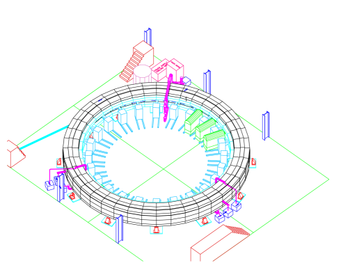
Figure 3: A 3D engineering rendition of the E821 muon storage ring. Muons enter the back of the storage ring through a field-free channel at approximately 10 o’clock in the figure. The three modules at approximately 2 o’clock provide the rapid current pulse which gives the muon bunch a transverse 10 mrad kick. The regularly spaced boxes on rails represent the electron detector systems.

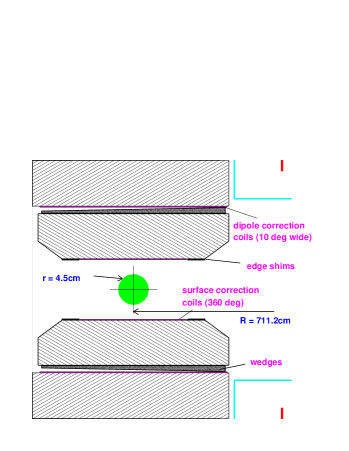
Figure 4: Slice of the storage ring magnet illustrating the key tools in the shimming kit and the relative size of the storage ring volume. The vacuum chamber, which encloses the storage volume and houses the quadrupoles and the trolley rails, is not shown.

Protons from the AGS strike a nickel target in 6–12 bunches separated by 33 ms within a typical 2.5–3.3 s AGS cycle. Pions created in these collisions are directed down a 72 m long beamline to the muon storage ring. Approximately half decay, $\pi\rightarrow\mu\nu$, and the forward going muons, having a high degree of longitudinal polarization, remain in the channel, generally at a slightly lower momentum. The last dipoles upstream of the entrance to the storage ring are tuned to a momentum $\approx 1.7\%$ lower than the main channel in order to enhance the muon fraction in the beam; the result is a final $\mu:\pi$ ratio of approximately $50:50$ entering the ring.

A superconducting inflector magnet $\!{}^{{\bf?}}$ provides a field-free channel through the back of the storage ring’s iron yoke. The field created by this magnet is tuned to cancel the main storage ring field. The inflector field is then prevented from extending into the storage ring by flux trapping in a superconducting outer shield.

The pulse structure of the AGS is translated to an effective muon bunch of approximately 25 ns $RMS$ passing through the exit of the inflector into the ring. A simple circular trajectory would result in the muon bunch striking the inflector magnet 149 ns after injection, which is the cyclotron period. A pulsed “kicker” magnet provides a 10 mrad transverse deflection to the muon bunch during the first turn in the ring. In practice, three pulsed magnets, all in series, are made from current sheets and special high-voltage pulsed power supplies.

The electric quadrupoles are located symmetrically at four positions occupying, in total, $43\%$ of the ring. Immediately after particle injection, the plates are asymmetrically charged in order to scrape the beam against internal collimaters. After approximately 20 $\mu$s, the voltages are symmetrized to final values of $\pm$24 kV which leads to the stored weak-focussing field index $n=0.137$. The horizontal and vertical betatron frequencies are $\omega_{x}\approx 6.23$ MHz and $\omega_{y}\approx 2.48$MHz, respectively. Because the inflector aperture is small compared to the cross-sectional area of the storage volume, phase space is not fully occupied and the stored beam exhibits “breathing” and “swimming” motions during a fill. These motions manifest themselves as effective modulations in the acceptance function of the detectors because the acceptance is sensitive, on average, to the position of the decaying muons. The relevance of this fact becomes clear when one realizes that the difference between the cyclotron and horizontal betatron frequencies is approximately 470 kHz, which is a little greater than twice $\omega_{a}$. These “coherent betatron oscillations” (CBO) are visible in the data; to account for CBO, Eq. 2 must be multiplied by a term of the type

$$C(t)=1+A_{cbo}e^{-(t/\tau_{cbo})^{2}}\cos(\omega_{cbo}t+\phi_{cbo})$$ (5)

where $\tau_{cbo}$ is the time constant for decay of the CBO terms having initial amplitude $A_{cbo}$.

3.2 Field Measurements

The magnetic field is measured using pulsed nuclear magnetic resonance (NMR) on protons in water- or Vaseline-filled probes. The proton precession frequency is proportional to the local field strength and is measured with respect to the same clock system employed in the determination of $\omega_{a}$. The absolute field is, in turn, determined by comparison with a precision measurement of $g_{p}$ in a spherical water sample $\!{}^{{\bf?}}$ and is thus determined to a precision of better than $10^{-7}$. A subset of the 360 “fixed” probes is used to continuously monitor the field during data taking. Fixed probes are embedded in machined grooves in the outer upper and lower plates of the aluminum vacuum chamber and consequently measure the field just outside of the actual storage volume. Constant field strength is maintained using 36 of the probes in a continuous feedback loop with the main magnet power supply.

The determination of the field inside the storage volume is made by use of a unique non-magnetic trolley which can travel in vacuum through the muon storage volume. The trolley carries 17 NMR probes on a grid appropriate to determine the local multipolarity of the field versus azimuth. Trolley field maps are made every few days and take several hours to complete. The deviation from the central field strength value $B_{0}=1.451266$ T versus azimuth is shown in Fig. 5. At any given location, field measurement precision is at the 0.1 ppm level even though the local field varies by as much as 100 ppm from $B_{0}$. However, it is the average field which must be determined to the sub ppm level and this goal is readily achieved. A 800 ppm “spike” in the field is seen in a $1^{\circ}$ azimuthal segment. This small defect is due to a crack in the inflector magnet shielding. Special measurements were made to map the field in this region for the 1999 data; this inflector was replaced for the 2000 and 2001 data taking periods. A one-time systematic error of 0.2 ppm is included in the 1999 result to account for uncertainties in the procedure of measuring the errant field in this region.

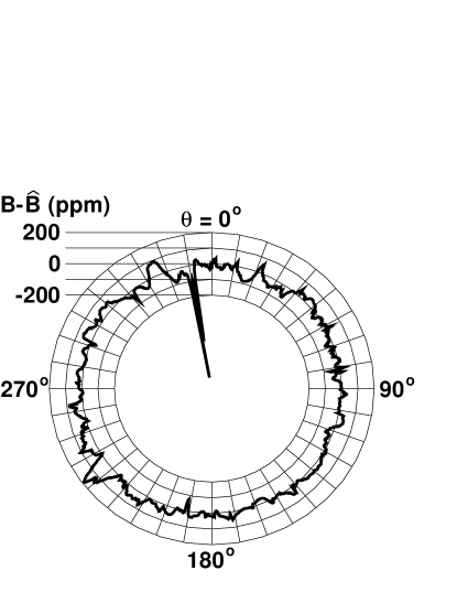
Figure 5: Magnetic field average versus azimuth from a typical trolley run. The spike at $350^{\circ}$ is due to a small crack in the inflector shielding which has since been repaired.

Comparison of the azimuthally averaged trolley field with that which is computed using the fixed probe data permits a determine of the time-dependent field. Figure 6 illustrates the excellent agreement between these two systems. The relative field is interpolated from the fixed-probe extrapolation to better than 0.15 ppm.

The trolley measurements also establish the field homogeneity throughout the storage volume. Three snapshots of the azimuthally-averaged field are shown in Fig. 7. The contours represent 1 ppm deviations from the central value. The left panel illustrates the relatively uneven field achieved shortly after the ring was commissioned in 1997; here it is already better than the CERN III field.$\!{}^{{\bf?}}$ An aggressive shimming program led to the improved contours for the 1998 and 1999 data taking periods (middle panel). With the inflector replaced, the field for the 2000 and 2001 data taking was again significantly improved (right panel).

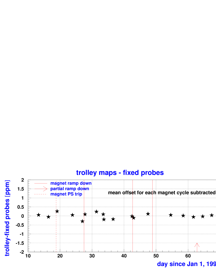
Figure 6: The magnetic field strength as measured at the center of the storage ring using the NMR trolley system compared to that which was expected from data obtained using the fixed NMR probes. Each point represents an individual trolly run during the 1999 data taking period. The agreement is at the 0.15 ppm level.

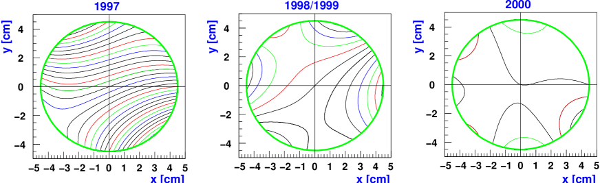
Figure 7: Sequence of improving magnetic field profiles, averaged over azimuth and interpolated using a multipole expansion. The circle indicates the storage aperture. From left to right, these maps represent the field variations for the 1997 commissioning run, the 1998/1999 data taking, and finally the 2000 run. Improvements in shimming and replacement of the inflector magnet led to the two major improvements following the 1997 and 1999 runs, respectively.

4 Electron Detection and $\omega_{a}$ Analysis

The electron detection system consists of 24 lead-scintillating fiber electromagnetic calorimeters $\!{}^{{\bf?}}$ located symmetrically around the inside of the storage ring and placed immediately adjacent to the vacuum chamber. The 23 cm long, radially-oriented fiber grid terminates on four lightguides which pipe the light to independent Hamamatsu R1828 2-inch PMTs, see Fig. 8. The PMT gains are carefully balanced because the four analog signals are added prior to sampling by a custom 400 MHz waveform digitizer. At least 16 digitized samples (usually 24 or more) are recorded for each decay electron event exceeding a hardware threshold of approximately 1 GeV. An example of a series of such samples is shown in Fig. 9. Offline pulse-finding and fitting establishes electron energy and muon time of decay.

Because the full raw waveforms are stored, multi-particle pileup can be studied with sophisticated fitting algorithms which are superior to any “online,” hardware discriminator techniques. The approach taken is to fit waveforms for all occurring pulses using known detector response functions. We identify the level of pileup and remove such events, on average. By processing the data using different artificial deadtime windows around or near the driving trigger pulse, and by carefully accounting for the energy found in such windows, a pileup-free spectrum (less than $10\%$ pileup remaining) can be created by appropriate, normalized difference spectra. Figure 10 illustrates three curves of the energy spectrum in the calorimeters. The solid curve is the “true” energy distribution found at late times where no pileup events are expected. The dashed distribution, which extends to much higher energies, is observed at early times when the rate in the detectors is high. Pileup produces effective electron energies beyond the natural maximum of 3.1 GeV. The dotted curve is the recreated pileup-free final spectrum. Its congruence with the late-time curve gives confidence in the correction procedure.

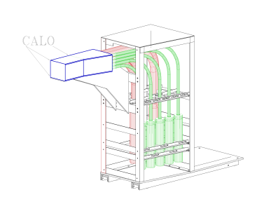
Figure 8: Electromagnetic calorimeter system for the experiment. The figure illustrates the four lightguides from the calorimeter and the five which couple to the scintillator hodoscope.

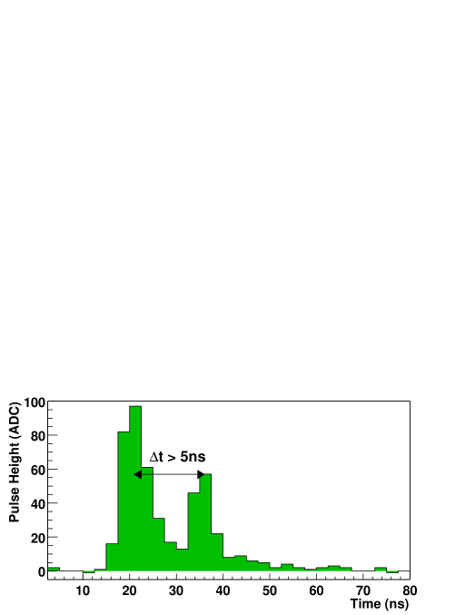
Figure 9: An “island” of waveform digitizer samples. In this representation, the constant offset has been subtracted. Two well-separated pulses are shown. The pulse-finding routines have no difficulty with such events. Special care is needed when the second pulse moves within 5 ns of the first event.

Figure 10: Energy spectrum at late times only (thin line), at all times (thick line) and after pileup subtraction (dashed line). The inset compares the average energy in a full $(g-2)$  cycle versus time for unsubtracted (solid circles) and subtracted (open circles) spectra. The energy distribution must be flat.

Five-fold, vertically segmented scintillator hodoscopes (FSDs) are attached to the front face of many of the calorimeters. These FSDs are used to measure the rate of “lost muons” from the storage ring. During the initial scraping period, and extending for a period of time afterwards, errant muon trajectories will pass through one of the aperature-defining collimaters inside the storage ring. These muons lose enough energy to exit the ring, many following a path which penetrates three consecutive calorimeters and their corresponding FSDs. A triple coincidence of FSDs, together with the absence of significant energy in the calorimeters, is proportional to the lost muon rate. A representative muon loss spectra for one detector is shown in Fig. 11 At early times, the loss rate exceeds the natural muon decay rate and can be described by an exponential with an approximate $27~{}\mu s$ lifetime. At later times, the loss rate is essentially constant. The overall loss rate is proportional to

$$\Lambda(t)=1+A_{\Lambda}e^{-t/\tau_{\Lambda}}.$$ (6)

Integration of $\Lambda(t)$ and inclusion in the fitting function is necessary to obtain a good representation of the instantaneous muon population in the ring.

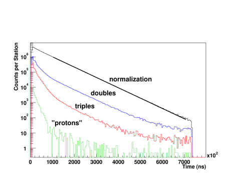
Figure 11: A muon loss distribution from one detector (1999 data). Binning in this histogram is in units of the $(g-2)$ period, thus the normalization curve is an exponential with lifetime of approximately 64 $\mu$s. The triples curve is proportional to the muon loss rate. After $\approx 100~{}\mu$s, the loss rate is essentially constant. At earlier times, the loss function is described by an exponential with a lifetime of approximately $27~{}\mu$s. The doubles curve is similar but, with a lower coincidence requirement, contains background. The “proton” curve involves three FSD coincidences and significant energy in the calorimeter of the third station. This occurs from occasional hadronic showers. The triples and doubles curves also show proton events at late times ($\approx 700\mu$s) when most muons have decayed.

5 Fitting the 1999 Data

The five adjustable parameters in Eq. 2 were sufficient to give an excellent $\chi^{2}$ when used to fit the 1998 data.$\!{}^{{\bf?}}$ Figure 12 illustrates data and 5-parameter fit for 1999. By eye, the fit also looks excellent; however, the $\chi^{2}$ is unacceptable because the CBO, pileup and muon losses have not been accounted for in this 20 times larger data set. The “pileup-free” spectrum is fit to the function

$$f(t)=N(t)\cdot C(t)\cdot\Lambda(t)$$ (7)

where $N(t)$ is the ideal function (Eq. 2), $C(t)$ accounts for the CBO (Eq. 5), and $\Lambda(t)$ characterizes the time-dependent muon lossses (Eq. 6). With Eq. 7, or equivalent fitting strategies used by the other analysis teams, $\chi^{2}$ is consistent with 1.

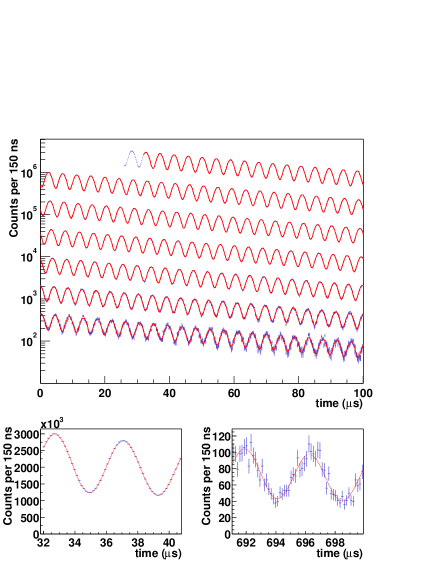
Figure 12: The 1999 data and a simple 5-parameter fit. While the fit looks good, see the lower panels, the $\chi^{2}$ is too high. A more complete fitting function, applied to a pileup-subtracted data set, yielded $\chi^{2}$ consistent with 1.

Deviations from the ideal function of the type described are more significant at early times compared to late times. One commonly used test employed by the analysis teams is to fit the data progressively beginning at different “start” times. As shown in Fig. 13, $\omega_{a}$ only fluctuates within the expected band but is otherwise stable. The distribution of variances from neighboring fits is shown on the lower right panel of the figure. This plot has a mean consistent with zero and a normalized width consistent with 1, as expected. The bottom left panels of the figure give $\omega_{a}$ and the $\chi^{2}$ by detector for the fixed start time of 30 $\mu$s. These and other statistical tests yield satisfactory results.

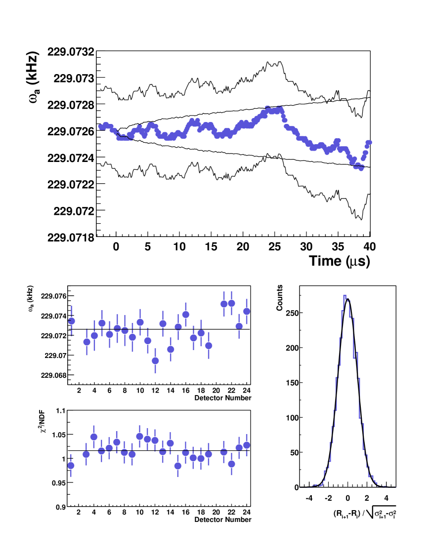
Figure 13: A series of “consistency” plots from one of the $\omega_{a}$ analyses. The top plot shows the stability of the fit for $\omega_{a}$ with respect to the start time of the fit. The solid bands represent the allowed $1\sigma$ deviation from the first fit point based on the understanding that later fits are highly correlated with the starting fit. The plot on the bottom right is the deviation of fit results for adjacent start times. It should be centered at zero with a width of 1 for deviations which are purely statistical. The panels on the lower left illustrate the stability of the fit versus detector number and the $\chi^{2}$ for each individual detector fit.

6 Results, Conclusions and Outlook

Table 1 summarizes the results. The experimental value from 1999 for positive muons is $a_{\mu^{+}}~{}=11\,659\,203(15)\times 10^{-10}$ (1.3 ppm. With the updated standard model theory value of $a_{\mu}(\rm{thy})=11~{}659~{}176.7(6.7)\times 10^{-10}$ (0.57 ppm), one finds $\Delta a_{\mu^{+}}(\rm{exp-thy})=25(16)\times 10^{-10}$. The 2000 $\mu^{+}$ data is presently being analyzed and should reduce the uncertainty considerably. The 2001 $\mu^{-}$ data is just beginning to be processed at the time of this writing. To complete the experiment, with equal positive and negative muon event samples, a final negative muon run will be necessary. The Collaboration is eager to complete this data taking phase and accompanying analysis in order to achieve our ultimate goal of 0.4 ppm precision or better in the measurement of the muon anomaly.

Item	Value	Relative Uncertainty
$\mbox{$\widetilde{\omega}_{p}$}/2\pi$	$61~{}791~{}256(25)$ Hz	0.4 ppm
$\mbox{$\omega_{a}$}/2\pi$	$229~{}072.8(3)$ Hz	1.3 ppm
Electric field correction	+0.81 ppm	$10\%$
Combined $\widetilde{\omega}_{p}$ systematic uncertainties	—	0.4 ppm
Combined $\omega_{a}$ systematic uncertainties	—	0.3 ppm
Final experimental value	$11\,659\,203(15)\times 10^{-10}$	1.3 ppm
Updated SM theory	$11~{}659~{}176.7(6.7)\times 10^{-10}$	0.57 ppm
$\Delta(a_{\mu^{+}}(\rm{exp-thy})$	$25(16)\times 10^{-10}$	$1.6~{}\sigma$

Table 1: Result summary for the 1999 data analysis.

References

References

- [1] The g-2 Collaboration for 1999: Boston U.: R.M. Carey, W. Earle, E. Efstathiadis, E.S. Hazen, F. Krienen, I. Logashenko, J.P. Miller, J. Paley, O. Rind, B.L. Roberts, L.R. Sulak, A. Trofimov; BNL: H.N. Brown, G. Bunce, G.T. Danby, R. Larsen, Y.Y. Lee, W. Meng, J. Mi, W.M. Morse, D. Nikas, C. Özben, C. Pai, R. Prigl, Y.K. Semertzidis, D. Warburton; Cornell U.: Y. Orlov; Fairfield U.: D. Winn; U. Heidelberg: A. Grossmann, K. Jungmann, G. zu Putlitz; U. Illinois: P.T. Debevec, W. Deninger, F.E. Gray, D.W. Hertzog, C.J.G. Onderwater, C. Polly, S. Sedykh, M. Sossong, D. Urner; Max Planck Heidelberg: U. Haeberlen; KEK: A. Yamamoto; U. Minnesota: P. Cushman, L. Duong, S. Giron, J. Kindem, I. Kronkvist, R. McNabb, C. Timmermans, D. Zimmerman; Budker I. Novosibirsk: V.P. Druzhinin, G.V. Fedotovich, B.I. Khazin, N.M. Ryskulov, Yu.M. Shatunov, E. Solodov; Tokyo I. Tech.: M. Iwasaki, M. Kawamura; Yale U.: H. Deng, S.K. Dhawan, F.J.M. Farley, V.W. Hughes, D. Kawall, M. Grosse Perdekamp, J. Pretz, S.I. Redin, E. Sichtermann, A. Steinmetz.
- [2] A. Czarnecki and W.J. Marciano, Nucl. Phys. B (Proc. Suppl.) 76, 245 (1999).
- [3] R.M. Carey et al., Phys. Rev. Lett. 82, 1632 (1999).
- [4] H.N. Brown et al., Muon Collaboration, Phys. Rev. D 62, 091101 (2000).
- [5] H.N. Brown et al., Phys. Rev. Lett. 86, 2227 (2001).
- [6] M. Knecht and A. Nyffeler (2001), hep-ph/0111058 and M. Knecht, A. Nyffeler, M. Perrottet, and E. de Rafael (2001), hep-ph/0111059.
- [7] M. Hayakawa and T. Kinoshita, Phys. Rev. D 57, 465 (1998).
- [8] J. Bijnens, E. Pallante, and J. Prades, Phys. Rev. Lett. 75, 1447 (1995).
- [9] M. Hayakawa and T. Kinoshita,hep-ph/0112102.
- [10] J. Bijnens, E. Pallante, and J. Prades, hep-ph/0112255; note, the sign error here enters from a completely different origin.
- [11] Simon Eidelman, these proceedings.
- [12] Andreas Höcker, Hadronic Contribution to , hep-ph/0111243 and these proceedings.
- [13] Kirill Melnikov, Int. J. Mod. Phys. A 16, 4591 (2001).
- [14] M. Davier and A. Höcker, Phys. Lett. B 435, 427 (1998).
- [15] S. Narison, Phys. Lett. B 513, 53 (2001), erratum: ibid. B526, 414 (2002).
- [16] J.F. de Trocóniz and F.J. Ynduráin, hep-ph/0106025.
- [17] William J. Marciano, these proceedings.
- [18] See, for example, the SPIRES citation search for Brown et al., (2001) above for hundreds of interesting examples of standard model extensions.
- [19] A written review by Francis Farley can be found in F.J.M. Farley and E. Picasso. Adv. Ser. Direct. High Energy Phys., 7 479 (1990).
- [20] D.E. Groom et al., Review of Particle Physics, Eur. Phys. J. C 15, 1 (2000).
- [21] G.T. Danby et al., Nucl. Inst. and Meth. A 457, 151 (2001).
- [22] F. Krienen, D. Loomba, and W. Meng, Nucl. Inst. and Meth. A 283, 5 (1989).
- [23] W.D. Phillips et al., Metrologia 13, 81 (1977); X. Fei, V.W. Hughes and R. Prigl, Nucl. Inst. and Meth. A 394, 349 (1997).
- [24] R. Prigl, U. Haeberlen, K. Jungmann, G. zu Putlitz and P. von Walter, Nucl. Inst. and Meth. A 374, 118 (1996).
- [25] J. Bailey, et al., Nucl. Phys. B 150, 1 (1979).
- [26] S. Sedykh, et al., Nucl. Inst. and Meth. A 455, 346 (2000).