Aaron Roodman
Stanford Linear Accelerator Center
Stanford, California, 94309.
(for the B AB AR Collaboration)

The BABAR experiment at the PEP-II asymmetric B factory at SLAC has collected a large sample of data at the $\mathchar 28935\relax(4S)$ resonance. I will summarize BABAR’s new results on CP violation, $B$ mixing and lifetimes, and a selection of rare $B$ decays. In particular, I will describe in detail the measurement of the CP violating parameter $\sin\!2\beta$; BABAR has observed CP violation in the neutral $B$ system finding $\sin\!2\beta=0.59\pm 0.14\pm 0.05$.

1 Introduction

There are four known manifestations of matter versus anti-matter asymmetry. The first is the observed lack of anti-matter in the universe. The second and third are the presence of CP violation in decays of the neutral Kaon, in mixing and in decays. The fourth is observation of CP violation in decays of the neutral $B$ meson, the primary subject of this paper. The fundamental goal of the BABAR experiment is to understand the relationship between these four observations.

CP violation is one of the conditions which must be present in the early universe to create the cosmological baryon asymmetry. One of the great ironies in particle physics is that the observed CP violation in the CKM matrix of the Standard Model of the charged-current weak interaction is too weak by many orders of magnitude to explain the baryon asymmetry. Thus the goal at BABAR is to discover whether the CKM matrix is the source of all CP violation in the $B$ meson. If there is a component of the observed CP violation which is not explained by the CKM matrix, then perhaps this extra component may play a role in the baryon asymmetry. In addition, there is presently no deeper understanding of the fundamental source of the CKM matrix, with its striking hierarchy of couplings, and a first step towards this is to thoroughly measure the size and phases of the quark’s weak couplings.

This paper will describe some of the recent results from the BABAR experiment. For results from the similar experiment in Japan, BELLE, operating at the KEK-B accelerator, please see the relevant paper in these proceedings.

1.1 CP Violation and the CKM Matrix

In the Standard Model the weak charged couplings between quarks are given by a 3x3 unitary matrix, the CKM Matrix. In this model all CP violation is due to a single complex phase in the CKM matrix. In the convenient parametrization due to Wolfenstein[1], the phase is placed in the $V_{td}$ and $V_{ub}$ elements; the phase of $V_{td}$ is $\beta$, and the phase of $V_{ub}^{*}$ is $\gamma$. Interference between $B^{0}$ mixing and decay allows us to measure $\sin\!2\beta$. A value of $\sin\!2\beta$ around 0.7 is expected from the constraints of measurements of CP violation in the neutral Kaon, $B_{d}$ and $B_{s}$ mixing, and the ratio $|V_{ub}/V_{cb}|$ using $b\rightarrow u$ and $b\rightarrow c$ semi-leptonic decays. Unfortunately, these measurements suffer from significant theoretical uncertainty. The ultimate goal is a precise measurement of several different manifestations of CP violation in the $B$ system.

1.2 PEP-II Asymmetric B Factory

The BABAR experiment operates at the PEP-II asymmetric $B$ factory at SLAC. This accelerator consists of two separate storage rings, with positrons at an energy of 3.1 GeV and electrons at 9.0 GeV, using the SLAC linac as an injector. PEP-II operates at the $\mathchar 28935\relax(4S)$ resonance, with the center-of-mass boosted by $\beta\gamma=0.55$ enabling BABAR to measure time dependent asymmetries. PEP-II has now surpassed its design luminosity goal of $3\times 10^{33}{\rm cm}^{-2}{\rm sec}^{-1}$, with typical peak luminosities of $4.2\times 10^{33}$. Recently the integrated luminosity has surpassed $240\mbox{\,fb}^{-1}$ per day. Design and typical parameters for PEP-II are shown in Table 1. The integrated luminosity over the course of the last two years is shown in Figure 1. All results, except for $\sin\!2\beta$, are based on a data sample of roughly $23\times 10^{6}$ $B\kern 1.79993pt\overline{\kern-1.79993ptB}{}$ decays. The $\sin\!2\beta$ result is based on a sample of $33\times 10^{6}$ $B\kern 1.79993pt\overline{\kern-1.79993ptB}{}$ decays.

Table 1: Design parameters and typical values for PEP-II.

Parameter	Design	Typical
$I_{e}^{+}$ (mA)	2140	1590
$I_{e}^{-}$ (mA)	750	950
$N_{Bunches}$	1658	728
Tune shift	0.03	0.07
Vertical Spot ($\mu m$)	5.4	5-6
Peak $\mathcal{L}$ ($10^{33}$)	3.0	4.2
Daily $\int\mathcal{L}$ ($\mbox{\,pb}^{-1}$)	135	240

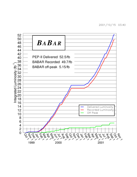
Figure 1: Integrated Luminosity as a function of time.

There are several important factors which allow PEP-II to achieve high luminosity. First, separate electron and positron rings allow high currents to be stored without disturbing the other beam. Second, having separate rings allows for the storage of many bunches, which permits high currents without large beam-beam tune shifts. In the simplest terms, the beam-beam tune shift describes the amount that a beam is perturbed by another beam. This tune shift is due to Coulomb interactions and is proportional to the number of particles in the other beam. An accelerator cannot function stably with too large a value of this tune shift[2]. Next, the use of numerous feedbacks makes stable operation at high luminosity possible. For example, PEP-II has single bunch feedbacks on the longitudinal and transverse position of every bunch, as well as slow feedbacks, of roughly 1-2 Hz, on the beam orbit, interaction angle, and luminosity itself.[3, 4] In practice the luminosity at PEP-II is limited by the amount of RF power available in each ring, and by beam-component heating, mostly from higher order RF modes.

1.3 BABAR Detector

The BABAR detector[5] is shown in Figure 2. The detector consists of a five layer double-sided silicon vertex detector (SVT), a 40 layer drift chamber (DCH), a cherenkov detector with quartz radiators and PMT readout (DIRC), a superconducting solenoid, a CsI(Tl) electromagnetic calorimeter (EMC), and an iron flux return instrumented with 19 layers of resistive plate chambers (IFR). The SVT has $15\mu m$ single hit resolution and the impact parameter resolution is $\sigma_{z}=65\mu m$ at 1 GeV. The DCH has a momentum resolution of $\sigma_{p_{t}}=0.13p_{t}+0.45\,\%$ and a dE/dx resolution of $8\%$ for high momentum electrons. The DIRC provides excellent particle identification, with $2.5\sigma$ K/$\pi$ separation at 4 GeV. The EMC has an energy resolution of $\sigma_{E}/E=1.85\oplus 2.32/\sqrt[4]{E}\,\%$. Finally, the IFR provides $\mu$ and $K^{0}_{\scriptscriptstyle L}$ identification.

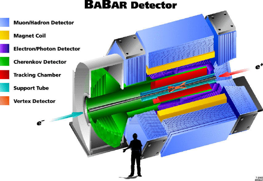
Figure 2: BABAR detector.

2 CP Violation Measurement

In this section, we will discuss in detail BABAR’s recent measurement of CP violation in the neutral $B$ meson.

2.1 CP Violation and Mixing in the $B$ meson

Typically CP violating amplitudes are measured through the interference of at least two amplitudes. In our case, the amplitude for the $B^{0}$’s decay to a final state which is also a CP eigenstate interferes with the amplitude for the $B^{0}$ to mix into a $\kern 1.79993pt\overline{\kern-1.79993ptB}{}^{0}$ and then decay into the same final state. The CP violating phase may occur in either the mixing amplitude for $B^{0}\leftrightarrow\kern 1.79993pt\overline{\kern-1.79993ptB}{}^{0}$ or the decay amplitude for $B^{0}\rightarrow f_{CP}$, or both.

The angle $\beta$ of the CKM matrix may be measured using the final state $b\rightarrow c\bar{c}s$; the dominant decay mode of this type is $B^{0}\rightarrow{J\mskip-3.0mu/\mskip-2.0mu\psi\mskip 2.0mu}K^{0}_{\scriptscriptstyle S}$. In the Wolfenstein parametrization, this decay amplitude has no phase, as seen in the tree-level diagram in Figure 3a. In addition there is a penguin diagram, shown in Figure 3b, which also has zero phase, for the dominant contribution with a top quark in the loop. Thus, unlike the case for other CP eigenstate final states, there is no extra interference between tree and penguin diagrams for $b\rightarrow c\bar{c}s$, and no appreciable theoretical uncertainty.

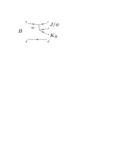
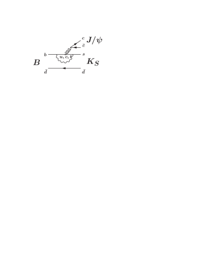
Figure 3: Feynman diagrams for $B^{0}\rightarrow{J\mskip-3.0mu/\mskip-2.0mu\psi\mskip 2.0mu}K^{0}_{\scriptscriptstyle S}$: a) tree level and b) penguin.

At the $\mathchar 28935\relax(4S)$ resonance we make $B^{0}$ mesons in correlated pairs, and both $B$ mixing and CP violating asymmetries depend on the decay time difference ${\rm\Delta}t$, not the absolute decay times. If both decay at the same time, then one must decay as a $B^{0}$ and the other as a $\kern 1.79993pt\overline{\kern-1.79993ptB}{}^{0}$. However, if the decay occurs at different times, then $B^{0}{\kern-1.60004pt\kern 1.79993pt\overline{\kern-1.79993ptB}{}^{0}}$ mixing may yield two $B^{0}$ or two $\kern 1.79993pt\overline{\kern-1.79993ptB}{}^{0}$ decays. Thus the CP violating asymmetry from the interference between mixing and decay amplitudes will increase as the mixing probability increases, and there will be no asymmetry at ${\rm\Delta}t=0$.

The time-dependent CP violation measurements are made with one decay to a CP eigenstate and the other to a flavor eigenstate. The decay rate is given by

$$f_{\pm}({\rm\Delta}t)=\frac{e^{-|{\rm\Delta}t|/\tau_{B^{0}}}}{4\tau_{B^{0}}}\times\left[1\pm(1-2\omega)\mathcal{I}m\lambda_{f_{CP}}\sin({\rm\Delta}m_{d}{\rm\Delta}t)\right]\otimes\mathcal{R}({\rm\Delta}t)$$ (1)

for $B^{0}$ and $\kern 1.79993pt\overline{\kern-1.79993ptB}{}^{0}$ flavor eigenstates. In the standard model $\lambda_{f_{CP}}=\pm e^{i2\beta}$ for $b\rightarrow c\bar{c}s$ decays. Here $\omega$, the mistag rate, is the probability of incorrectly identifying the flavor eigenstate, and $\mathcal{R}$ is the ${\rm\Delta}t$ resolution function. The $B^{0}$ mixing measurements are made with both $B^{0}$ decaying into flavor eigenstates. The decay rate is given by

$$f_{\pm}({\rm\Delta}t)=\frac{\exp{-|{\rm\Delta}t|/\tau_{B^{0}}}}{4\tau_{B^{0}}}\times\left[1\pm(1-2\omega)\cos{{\rm\Delta}m_{d}{\rm\Delta}t}\right]\otimes\mathcal{R}({\rm\Delta}t)$$ (2)

for un-mixed and mixed events, and where ${\rm\Delta}m_{d}$ is the mass difference between the CP Eigenstates $B_{H}$ and $B_{L}$. Since the mistag rate and the ${\rm\Delta}t$ resolution function can be measured directly using the mixing sample, the CP asymmetry measurement is immune from most systematic uncertainties.

2.2 Elements of the CP Violation Measurement

To measure $\sin\!2\beta$ we identify a sample of decays of the sort $B^{0}\rightarrow{J\mskip-3.0mu/\mskip-2.0mu\psi\mskip 2.0mu}K^{0}_{\scriptscriptstyle S}$, determine the flavor of the other $B^{0}$ through its decay into a flavor eigenstate, and measure the time difference ${\rm\Delta}t$ between the two decays. In the center-of-mass typically ${\rm\Delta}z\sim 30\mu m$, but the asymmetric collider boosts this to ${\rm\Delta}z\sim 260\mu m$ in the lab frame, which is roughly twice the vertex resolution. The effectiveness of the flavor determination and the vertex resolution function are both determined by using a large sample of exclusively reconstructed decays into flavor eigenstates.

2.2.1 Data Samples

There are several decay modes which are used to amass a sample of $b\rightarrow c\bar{c}s$ events, which comprise our CP data sample. The $c\bar{c}$ quarks make either a ${J\mskip-3.0mu/\mskip-2.0mu\psi\mskip 2.0mu}$, $\psi(2S)$, or $\chi_{c1}$. For the ${J\mskip-3.0mu/\mskip-2.0mu\psi\mskip 2.0mu}$ we use only the decay into electron or muon pairs. The $\psi(2S)$ decay into lepton pairs and that into ${J\mskip-3.0mu/\mskip-2.0mu\psi\mskip 2.0mu}\pi^{+}\pi^{-}$ are used. The $\chi_{c1}$ decay into ${J\mskip-3.0mu/\mskip-2.0mu\psi\mskip 2.0mu}\gamma$ is used. The $s$ quark hadronizes into a $K^{0}_{\scriptscriptstyle S}$, $K^{0}_{\scriptscriptstyle L}$, or a $K^{*}$. Of course only the decays of the $K^{*}$ into neutral kaons can be used. Both charged and neutral two pion decays of the $K^{0}_{\scriptscriptstyle S}$ are used. The $K^{0}_{\scriptscriptstyle L}$ are detected directly in the EMC and the IFR.

Reconstructed ${J\mskip-3.0mu/\mskip-2.0mu\psi\mskip 2.0mu}$, $\psi{(2S)}$, and $\chi_{c1}$ are combined with reconstructed $K^{0}_{\scriptscriptstyle S}$, $K^{0}_{\scriptscriptstyle L}$, or $K^{*}$ to make up a $B^{0}$. The $K^{0}_{\scriptscriptstyle L}$ mode has only one independent kinematic variable since one constraint must be used to infer the $K^{0}_{\scriptscriptstyle L}$ momentum; only the $K^{0}_{\scriptscriptstyle L}$ direction is measured in the IFR. The energy substituted $B$ mass, $\mbox{$m_{\rm ES}$}=\sqrt{E_{\rm Beam}^{2}-p_{B}^{2}}$ and $\Delta E=E_{B^{0}}-E_{\rm Beam}$ are shown in Figure 4 for a sample of $33\times 10^{6}$ $B\kern 1.79993pt\overline{\kern-1.79993ptB}{}$ events taken during 1999-2001. There was a significant improvement in the reconstruction efficiency of the 2001 data compared to that of the 2000 year data, due mostly to improved DCH tracking reconstruction for $K^{0}_{\scriptscriptstyle S}\rightarrow\pi^{+}\pi^{-}$. This improvement will be applied to the data from 1999-2000 when that data set is eventually re-analyzed.

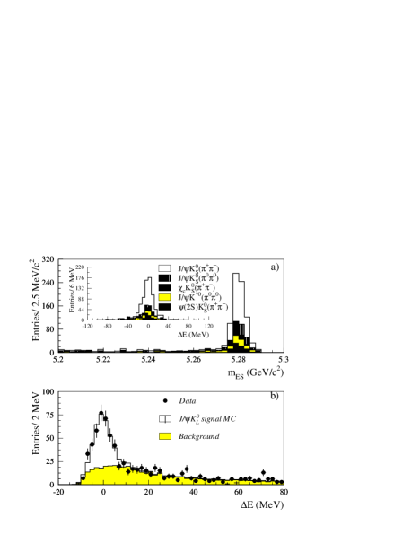
Figure 4: a) $m_{\rm ES}$ and $\Delta E$ distributions for the CP=-1 data sample (the $B^{0}\rightarrow{J\mskip-3.0mu/\mskip-2.0mu\psi\mskip 2.0mu}K^{*}$sample is a mix of CP=-1 and CP=+1, but it is used as a CP=-1 state with an extra dilution factor of 0.7), and b) $\Delta E$ for the CP=+1 sample.

2.2.2 B Flavor Tagging

The flavor of the other $B^{0}$ is determined from the charge of high momentum leptons, kaons, and slow pions from $D^{*}$ decays. Electrons are identified using the ratio of EMC energy and track momentum, the shower shape in the EMC, the $dE/dx$ in the DCH, and the cherenkov angle in the DIRC. The efficiency and mis-identification rate for electrons are shown in Figure 5a. Muons are identified using the hits in the IFR, and by comparing the DCH track’s extrapolation through the IFR with the IFR hits. The efficiency and mis-identification rate from pions are shown in Figure 5b. The mis-identification rate is somewhat higher than desired due mostly to the thickness, 4.5 to 6.0 interaction lengths, of the detector, and to inefficiencies in the RPCs. Charged kaons are identified using the $dE/dx$ in the SVT and DCH, the cherenkov angle and number of cherenkov photons in the DIRC. There is good separation between kaons and pions up to around 0.6 GeV from dE/dx and the cherenkov threshold in the DIRC is approximately 0.6 GeV, so there is good Kaon identification for all momentum. The Kaon efficiency and mis-identification for pions are shown in Figure 5c.

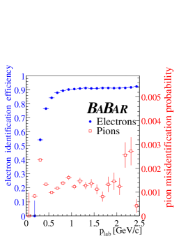
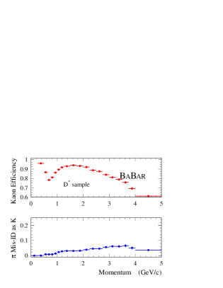
Figure 5: Particle identification at BABAR a) electrons, b) muons, c) kaons. The efficiency and mis-identification probability is shown as a function of momentum.

To determine the flavor of the $B^{0}$, each event is categorized, or tagged, according to its particle content. First, events with electrons with $p_{CM}>1.0~{}GeV$ and muons with $p_{CM}>1.1~{}GeV$ are used in the Lepton category. Next, events with one or more charged kaons are used in the Kaon category. For multiple kaons, the sum of Kaon charge is used. An artificial neural network is used for all remaining events. The neural network uses slow pions from $D^{*}$ decays and any remaining leptons or charged kaons which fail their respective selection. Slow pions are identified by their $p_{CM}$ and the angle between the pion and the thrust axis of all tracks and neutral EMC clusters from the $B^{0}$. This thrust axis is generally aligned with the original $D^{*}$ direction, as is the slow pion direction. Additional leptons are identified using the lepton momentum and the lepton’s isolation with respect to other tracks and clusters from the other $B^{0}$. Two categories are defined from the output of the neural network, NT1 and NT2, corresponding to more certain and less certain events.

The efficiency and mistagging rates are determined from the $B^{0}$ mixing sample in which one $B^{0}$ is fully reconstructed in a flavor eigenstate. By using data to measure the efficiency and mistag rates, most systematic effects are canceled. A sample of decays $B^{0}\rightarrow D^{*}n\pi$, $B^{0}\rightarrow Dn\pi$, and $B^{0}\rightarrow{J\mskip-3.0mu/\mskip-2.0mu\psi\mskip 2.0mu}K^{*},K^{*}\rightarrow K^{\pm}\pi$ are used for the flavor eigenstate sample; the $m_{\rm ES}$ for this sample is shown in Figure 6. The tagging efficiency and mistag rates are shown in Table 2, along with the quality factor $Q=\epsilon(1-2\omega)^{2}$. The statistical power of the asymmetry measurement is given by $\sigma_{\rm asym}=\sigma_{0}/\sqrt{(NQ)}$.

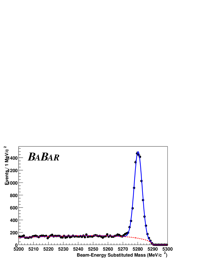
Figure 6: $m_{\rm ES}$ for the exclusively reconstructed $B^{0}$ sample.

Table 2: Tagging efficiency, mistag rate, and quality factor $Q$ from the flavor eigenstate sample.

Category	$\epsilon(\%)$	$\omega(\%)$	$Q(\%)$
Lepton	$10.9\pm 0.3$	$8.9\pm 1.3$	$7.4\pm 0.5$
Kaon	$35.8\pm 0.5$	$17.6\pm 1.0$	$15.0\pm 0.9$
NT1	$7.8\pm 0.3$	$22.0\pm 2.1$	$2.5\pm 0.4$
NT2	$13.8\pm 0.3$	$35.1\pm 1.9$	$1.2\pm 0.3$
Total	$68.4\pm 0.7$		$26.1\pm 1.2$

2.2.3 B Vertex and Decay Time

The decay time difference ${\rm\Delta}t$ is measured using the SVT to determine the ${\rm\Delta}z$ between the two $B^{0}$ decays. We convert according to ${\rm\Delta}t={\rm\Delta}z/(c\beta\gamma)$ with a correction for the deviation of the $B$ flight direction from the beam axis. The vertex of the exclusively reconstructed CP or Flavor decay is determined by a constrained fit of the measured tracks, taking into account the presence of intermediate decay particles such as $D^{0}$ and $K^{0}_{\scriptscriptstyle S}$. For the other $B^{0}$, which is not fully reconstructed, the vertex finding is complicated by the fact that long-lived intermediate particles are not identified, and the vertex is susceptible to a bias from $D^{0}$ or $K^{0}_{\scriptscriptstyle S}$ decays. To avoid such bias, tracks which contribution too much to the vertex $\chi^{2}$ are iteratively removed from the vertex fit. Also, to further improve the vertex measurements, and to allow the use of events in which there is only one charged track, the ${\rm\Delta}z$ is determined using a constraint derived from the exclusive $B^{0}$ direction and the beam spot. The overall ${\rm\Delta}z$ resolution is $190\,\mu\rm m$, with a core resolution of $110\mu m$ comprising roughly 65% of the events.

The ${\rm\Delta}t$ resolution function is parametrized as the sum of three Gaussian distributions. Roughly speaking the first Gaussian is for the core of the distribution, the second for the multiple scattering tail, and the third is nearly flat to account for mis-measured events. As part of the parametrization, the estimated error for each event from the ${\rm\Delta}z$ fit is used. Decays with higher track multiplicity and higher $p_{T}$ tracks have smaller $\sigma_{{\rm\Delta}z}$. The resolution function parametrization is given by

$$\mathcal{R}({\rm\Delta}t)=\sum_{\mathrm{core,tail}}\frac{1}{\sqrt{2\pi}S_{i}\sigma_{{\rm\Delta}t}}e^{-\frac{({\rm\Delta}t-m_{i,c}\sigma_{{\rm\Delta}t})^{2}}{2(S_{i}\sigma_{{\rm\Delta}t})^{2}}}+\frac{1}{\sqrt{2\pi}\sigma_{\mathrm{outlier}}}e^{-\frac{({\rm\Delta}t)^{2}}{2(\sigma_{\mathrm{outlier}})^{2}}}$$ (3)

where the estimated error for each event, $\sigma_{{\rm\Delta}t}$, are scaled by free parameters $S_{i}$, and an offset to account for remaining bias from charm meson decays is parametrized with a linear dependence on the estimated error. The sample of exclusively reconstructed $B^{0}$ is used, in the combined fit described below, to determine the values of the free parameters.

2.3 CP Violation Results

The CP violating asymmetry is measured using an unbinned maximum likelihood fit. The likelihood function for signal events is simply the expression given for the decay rate. To easily include the statistical uncertainty from the flavor tagging and vertex resolution parametrization, we use a combined fit to both the CP events and the Flavor events.

In addition, to help avoid experimenters bias, the CP fit is done blind to the value of $\sin\!2\beta$. Prior to finalizing the measurement, the asymmetry parameter used in the fit was

$$a^{\mathrm{Hidden}}=\left\{\begin{array}[]{c}1\\ -1\end{array}\right\}\times a+C$$ (4)

where the value of $C$ and the choice of 1 or -1 was fixed, arbitrary and hidden. To also hide any visual asymmetry, the ${\rm\Delta}t$ distribution was altered in plotting by ${\rm\Delta}t^{\mathrm{Hidden}}=\mathrm{S}_{\rm Tag}{\rm\Delta}t+\mathrm{Offset}$, where again the $\mathrm{Offset}$ was fixed, arbitrary and hidden. The asymmetry result was hidden until the analysis was essentially complete.

The ${\rm\Delta}t$ distribution for $B^{0}$ and $\kern 1.79993pt\overline{\kern-1.79993ptB}{}^{0}$ tags is shown in Figure 7 for the $CP=-1$ decays modes $B^{0}\rightarrow{J\mskip-3.0mu/\mskip-2.0mu\psi\mskip 2.0mu}K^{0}_{\scriptscriptstyle S}$, $B^{0}\rightarrow\psi{(2S)}K^{0}_{\scriptscriptstyle S}$, and $B^{0}\rightarrow\chi_{c1}K^{0}_{\scriptscriptstyle S}$ and the $CP=+1$ mode $B^{0}\rightarrow{J\mskip-3.0mu/\mskip-2.0mu\psi\mskip 2.0mu}K^{0}_{\scriptscriptstyle L}$. Also shown is the raw asymmetry as a function of the ${\rm\Delta}t$. The $\sin$ oscillation is readily apparent. We find a value for $\sin\!2\beta$ of[6]

$$\sin\!2\beta=0.59\pm 0.14(\textrm{stat})\pm 0.05(\textrm{syst})$$ (5)

The systematic error is largely due to uncertainties in the ${\rm\Delta}z$ determination and the mistagging probability, with smaller contributions from uncertainty in the values of ${\rm\Delta}m_{d}$ and $\tau_{B^{0}}$. The $B^{0}\rightarrow{J\mskip-3.0mu/\mskip-2.0mu\psi\mskip 2.0mu}K^{0}_{\scriptscriptstyle L}$ has an additional systematic contribution from its larger background.

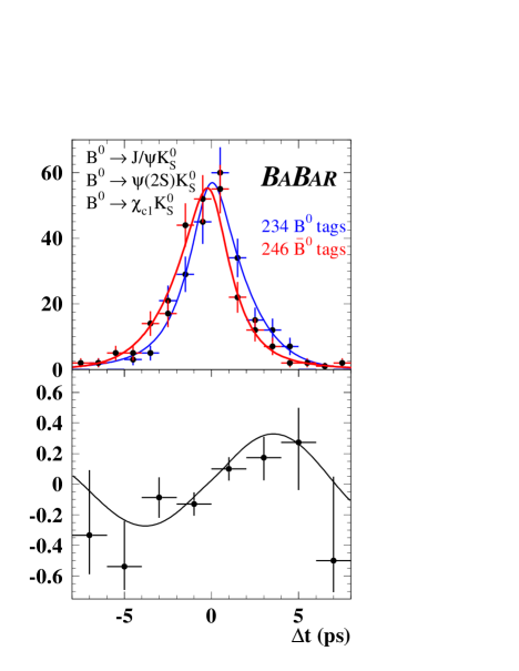
Figure 7: The ${\rm\Delta}t$ distribution for $B^{0}$ and $\kern 1.79993pt\overline{\kern-1.79993ptB}{}^{0}$ tags and the Asymmetry, $\mathcal{A}({\rm\Delta}t)=(N_{B^{0}}-N_{\kern 1.25995pt\overline{\kern-1.25995ptB}{}^{0}})/(N_{B^{0}}+N_{\kern 1.25995pt\overline{\kern-1.25995ptB}{}^{0}})$ for a) the CP=-1 sample ($K^{0}_{\scriptscriptstyle S}$ decays), and b) the CP=+1 sample($K^{0}_{\scriptscriptstyle L}$ decays).

Our measured value of $\sin\!2\beta$ and the constraints from other measurements are shown in Figure 8

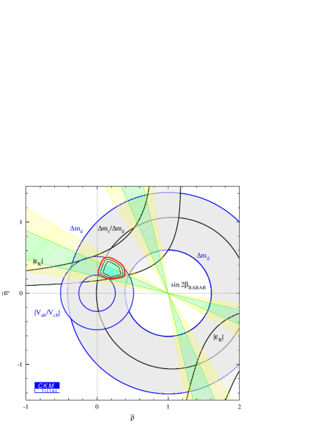
Figure 8: BABAR measurement of $\sin\!2\beta$ in the CKM $\rho-\eta$ plane, along with constraints from other measurements.

At the level of the statistical uncertainty in $\sin\!2\beta$ there is good agreement among the measurements in the $\rho-\eta$ plane. As the measurement of $\sin\!2\beta$ improves statistically, the comparison will depend heavily on the theoretical uncertainties in translating measurements of $b\rightarrow ul\nu$, ${\rm\Delta}m_{d}$, and $\epsilon_{K}$ into CKM parameters. When ${\rm\Delta}m_{s}$ mixing is measured, the theoretical uncertainty will decrease by using the ratio ${\rm\Delta}m_{s}/{\rm\Delta}m_{d}$, and improvement is possible in $|V_{ub}|$ given more data and expected improvements in lattice calculations. However, a test of the entire CKM picture at the 5% level will likely require an accurate and theoretically clean measurement of one of the other CP violating angles.

3 B Lifetime and Mixing

A measurement of the fundamental parameters of the $B$ meson system, the $B^{0}$ and $B^{\pm}$ lifetimes, and the $B^{0}$ mixing parameter ${\rm\Delta}m_{d}$, provide crucial input to the CP asymmetry measurements and to the constraints on the parameters of the CKM matrix.

3.1 B Lifetime Measurement

The $B^{0}$ and $B^{\pm}$ lifetimes are measured with a sample of exclusively reconstructed decays. The ${\rm\Delta}t$ distribution of the 6967 $B^{0}$ and 7266 $B^{\pm}$ events is shown in Figure 9. The resolution function is parametrized in a somewhat different way than in the CP violation measurement, using a Gaussian+Exponential convolution. As in the asymmetry measurement, an unbinned maximum likelihood fit is performed. The results for the lifetimes[7] are listed in Table 3. where the systematic uncertainty comes from the outlier contribution to the resolution function (0.011), resolution parameterization (0.011), and absolute Z scale (0.008). Systematic for the lifetime ratio come from differences in the resolution function for $B^{0}$ and $B^{\pm}$ (0.006), and outliers (0.005).

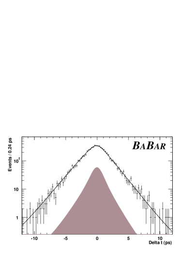
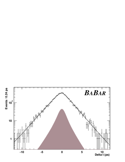
Figure 9: The ${\rm\Delta}t$ distributions for a) $B^{0}$ and b) $B^{\pm}$ decays, along with the fit for the lifetime.

The ratio $\tau_{\pm}/\tau_{0}$ is sensitive to the $B$ decay constant, $f_{B}$, due to the contribution from W-exchange diagrams which occur for $B^{0}$ decay only.

Table 3: Results from the BABAR Experiment.

Quantity	Result
$\tau_{B^{0}}$	$1.546\pm 0.032({\rm stat})\pm 0.022({\rm syst}){\rm\,ps}$
$\tau_{B^{\pm}}$	$1.673\pm 0.032({\rm stat})\pm 0.022({\rm syst}){\rm\,ps}$
$\tau_{B^{\pm}}/\tau_{B^{0}}$	$1.082\pm 0.026({\rm stat})\pm 0.012({\rm syst})$
${\rm\Delta}m_{d}$ Exclusive	$0.519\pm 0.020(\mathrm{stat})\pm 0.016(\mathrm{syst}){\rm\,ps}^{-1}$
${\rm\Delta}m_{d}$ dilepton	$0.499\pm 0.010(\mathrm{stat})\pm 0.012(\mathrm{syst}){\rm\,ps}^{-1}$
$\mathcal{B}(B^{0}\rightarrow K^{*0}\gamma)$	$(4.39\pm 0.42(\mathrm{stat})\pm 0.27(\mathrm{syst}))\times 10^{-5}$
$A_{CP}$ $K^{*0}\gamma$	$-0.035\pm 0.094(\mathrm{stat})\pm 0.022(\mathrm{syst})$
$\mathcal{B}(B^{0}\rightarrow\pi^{+}\pi^{-})$	$(4.1\pm 1.0(\mathrm{stat})\pm 0.7(\mathrm{syst}))\times 10^{-6}$
$\mathcal{B}(B^{0}\rightarrow K^{\pm}\pi^{\mp})$	$(16.7\pm 1.6(\mathrm{stat})\pm^{+1.2}_{-1.7}(\mathrm{syst}))\times 10^{-6}$
$\mathcal{B}(B^{0}\rightarrow K^{\pm}K^{\mp})$	$<2.5\times 10^{-6}$
$A_{CP}$ $K\pi$	$-0.19\pm 0.10(\mathrm{stat})\pm 0.03(\mathrm{syst})$
$\mathcal{B}(B^{\pm}\rightarrow\phi K^{\pm})$	$(7.7^{+1.6}_{-1.4}(\mathrm{stat})\pm 0.8(\mathrm{syst}))\times 10^{-6}$
$\mathcal{B}(B^{0}\rightarrow\phi K^{0}_{\scriptscriptstyle S})$	$(8.1^{+3.1}_{-2.5}(\mathrm{stat})\pm 0.8(\mathrm{syst}))\times 10^{-6}$
$\mathcal{B}(B^{\pm}\rightarrow\phi K^{*\pm})$	$(9.6^{+4.1}_{-3.3}(\mathrm{stat})\pm 1.7(\mathrm{syst}))\times 10^{-6}$
$\mathcal{B}(B^{0}\rightarrow\phi K^{*0})$	$(8.6^{+2.8}_{-2.4}(\mathrm{stat})\pm 1.1(\mathrm{syst}))\times 10^{-6}$

3.2 B Mixing Measurement

The $B^{0}$ mixing parameter ${\rm\Delta}m_{d}$ has been measured using two different samples. The first is the exclusively reconstructed sample used in the CP asymmetry measurement, and the second is a sample of events in which both $B^{0}$ decay semi-leptonically.

3.2.1 Mixing in Exclusive Decays

The $B^{0}$ mixing parameter ${\rm\Delta}m_{d}$ is measured using the exclusively reconstructed sample and the inclusive flavor tagging of the other $B^{0}$ to determine the fraction of mixed $B^{0}B^{0}$ or $\kern 1.79993pt\overline{\kern-1.79993ptB}{}^{0}\kern 1.79993pt\overline{\kern-1.79993ptB}{}^{0}$ events. The asymmetry between mixed and un-mixed events is given by

$$\mathcal{A}_{\rm mixing}({\rm\Delta}t)=(\textrm{Mixed}-\textrm{Un-Mixed})/(\textrm{Mixed}+\textrm{Un-Mixed})=(1-2\omega)\cos{({\rm\Delta}m_{d}{\rm\Delta}t)}$$ (6)

As in the CP measurement, the asymmetry is modified by incorrect flavor tagging and vertex resolution and the value of ${\rm\Delta}m_{d}$ is again found from an unbinned maximum likelihood fit. The ${\rm\Delta}t$ distribution is shown in Figure 10 along with the asymmetry as a function of ${\rm\Delta}t$. The preliminary value is listed in Table 3[8]. The systematic uncertainties are due to corrections taken from simulation (0.009), the ${\rm\Delta}t$ measurement scale, boost, and alignment uncertainty (0.008), $B^{0}$ lifetime (0.006), and backgrounds (0.005).

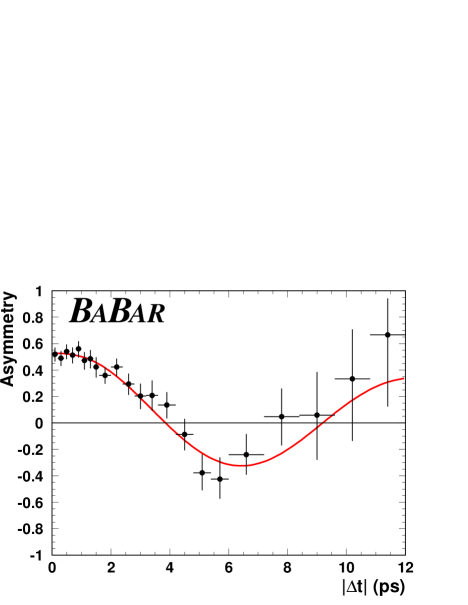
Figure 10: The $B^{0}$ mixing asymmetry as a function of ${\rm\Delta}t$, with the fit from ${\rm\Delta}m_{d}$ for the exclusively reconstructed sample.

3.2.2 Mixing in Di-Lepton Decays

Alternatively the $B^{0}$ mixing parameter can be measured with a sample of events in which both $B^{0}$ decay semileptonically. Compared with the exclusively reconstructed sample above, the use of semi-leptonic decays supplies more events, with greater backgrounds. In semi-leptonic events $B^{\pm}$ decays cannot be fully separated from $B^{0}$ decays, and these extra events dilute the mixing asymmetry. In addition there are backgrounds from cascade decays, $b\rightarrow c\rightarrow l$. The mixing asymmetry is given by

$$\mathcal{A}({\rm\Delta}t)=(1-2\omega)\frac{e^{-\Gamma^{0}|{\rm\Delta}t|}\cos{({\rm\Delta}m_{d}{\rm\Delta}t)}+R\frac{\Gamma^{\pm}}{\Gamma^{0}}e^{-\Gamma^{\pm}|{\rm\Delta}t|}}{e^{-\Gamma^{0}|{\rm\Delta}t|}+R\frac{\Gamma^{\pm}}{\Gamma^{0}}e^{-\Gamma^{\pm}|{\rm\Delta}t|}}$$ (7)

where $\omega$ is the mistag Probability and $R=\frac{b_{+}^{2}f_{\pm}}{b_{0}^{2}f_{00}}$ is the ratio of semi-leptonic branching ratios and production rates for $B^{0}$ and $B^{\pm}$. The ratio $R$ is fit from the data to avoid systematic uncertainty from the lack of sufficiently accurate measurements.

The mixing asymmetry is shown in Figure 11. The preliminary result is listed in Table 3. The systematic uncertainties arise mostly from the $\Delta z$ resolution function (0.009), cascade backgrounds (0.006) and dependence on the $B^{0}$ and $B^{\pm}$ lifetimes (0.004).

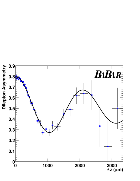
Figure 11: The $B^{0}$ mixing asymmetry as a function of ${\rm\Delta}t$, with the fit from ${\rm\Delta}m_{d}$ for the di-lepton sample.

These measurements of ${\rm\Delta}m_{d}$ have an accuracy comparable to the previous world average. When combined with an equally accurate measurement of ${\rm\Delta}m_{s}$ they will provide a theoretically clean constraint on the CKM matrix.

4 Rare B Decays

The bulk of $B$ decays are examples of the quark level process $b\rightarrow cW$, and the CP asymmetry and $B^{0}$ mixing measurements described above use decays of this type. However, to measure the unitarity triangle angles $\alpha$ or $\gamma$ will require measurements of the Cabibbo suppressed decay $b\rightarrow uW$. Also rare decays involving loop diagrams, commonly called penguin diagrams, offer the potential to detect the influence of non-Standard Model physics on $B$ decays. Here we present several BABAR branching fraction and direct CP asymmetry measurements for such rare decays.

As in any rare decay, the challenge in measuring rare $B$ meson decay modes lies in separating signal from background. For decays which are exclusively reconstructed, there are two kinematic variables which are effective in separating $B$ decays from backgrounds. At BABAR we typically use the $B$ mass and energy as our kinematic variables. A pair of nearly independent variables are:

$$\mbox{$m_{\rm ES}$}=\sqrt{(E_{\rm beam}^{CM})^{2}-(p^{CM}_{B^{0}})^{2}}\hskip 28.45274pt\Delta E=E_{B^{0}}^{CM}-E_{\rm beam}^{CM}.$$ (8)

We use the difference in measured energy and beam energy to remove any variations in the beam energy. Then the beam energy is substituted in the mass variable $m_{\rm ES}$ to remove most of the correlation between $m_{\rm ES}$ and $\Delta E$, and to improve its resolution. The resolution of $m_{\rm ES}$ is generally dominated by the beam energy spread of order 2.5 MeV, while the detector resolution dominates $\Delta E$.

4.1 Radiative Penguin Decays

Decays of the type $B\rightarrow K^{*}\gamma$ can only occur through radiative penguin decays, with the diagram shown in Figure 12a.

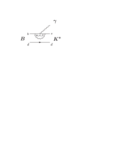
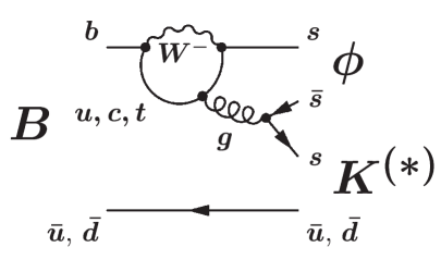
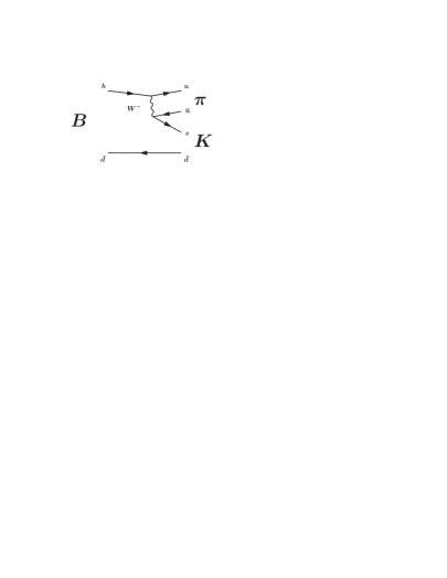
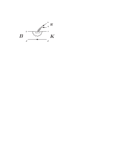
Figure 12: Feynman diagrams for a) $B\rightarrow K^{*}\gamma$, b) $B\rightarrow\phi K$, c) $B^{0}\rightarrow K^{\pm}\pi^{\mp}$tree-level, and d) $B^{0}\rightarrow K^{\pm}\pi^{\mp}$penguin.

Backgrounds to this decay arise from continuum $q\bar{q}$ events with a leading $\pi^{0}$ or $\eta$ and from events with a high momentum $\gamma$ from initial state radiation. Event shape variables are effective in separating these backgrounds from $B$ decays. The signal for the decay $B^{0}\rightarrow K^{*0}\gamma$ and $K^{*0}\rightarrow K^{+}\pi^{-}$ is shown in Figure 13. With a signal of $139.2\pm 13.1$ events, BABAR finds the branching fraction[9] tabulated in Table 3. The systematics on the asymmetry are due to limits for charged Kaon sign asymmetries in the detector. More data will be needed to accurately search for the small expected CP asymmetries.

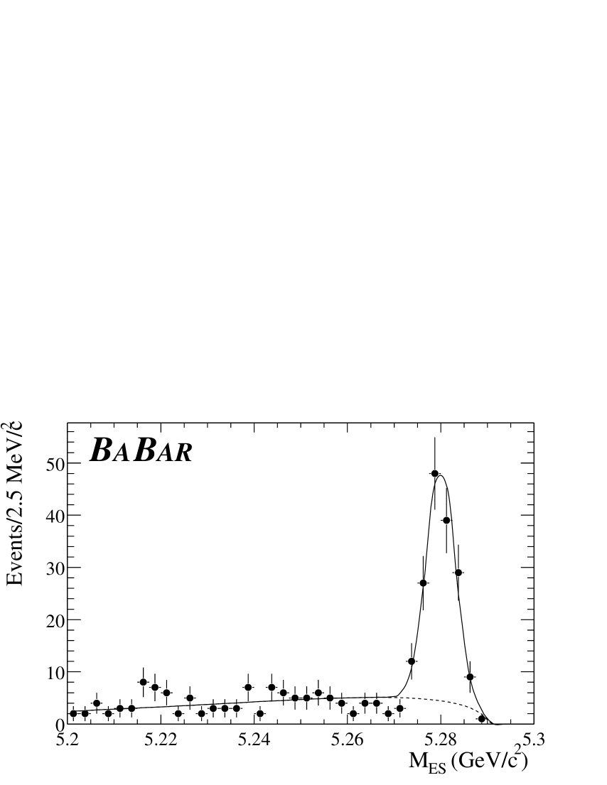
Figure 13: $m_{\rm ES}$ for the decay $B^{0}\rightarrow K^{*0}\gamma$.

4.2 Charmless Decays

The angle $\alpha$ of the CKM unitarity triangle can potentially be measured in the the time dependent asymmetry in $B^{0}\rightarrow\pi^{+}\pi^{-}$. Unfortunately, this asymmetry will be difficult to interpret, due to competing contributions from tree-level and penguin diagrams, shown in Figure 12b and c. However, this confusion might be resolved with theoretical input, or by measuring the $B^{0}$ and $\kern 1.79993pt\overline{\kern-1.79993ptB}{}^{0}$ rates for the decay $B^{0}\rightarrow\pi^{0}\pi^{0}$. The first step is to accumulate a sample of $B^{0}\rightarrow\pi^{+}\pi^{-}$ decays.

Observation of $B^{0}\rightarrow\pi^{+}\pi^{-}$ is also complicated by the need to separate $\pi\pi$ and $K\pi$ decays. BABAR’s DIRC was designed to provide excellent $K/\pi$ separation for these decay modes. The DIRC’s $K/\pi$ separation can be seen in Figure 14 from a sample of $D^{0}\rightarrow K^{\pm}\pi^{\mp}$ decays. The DIRC’s response, an event shape variable, and the kinematic variables $m_{\rm ES}$ and $\Delta E$ are combined in an unbinned maximum likelihood fit to the rate for both $B^{0}\rightarrow\pi^{+}\pi^{-}$ and $B^{0}\rightarrow K^{\pm}\pi^{\mp}$. The branching fraction results[10], are listed in Table 3. Often it is difficult to visualize the signal detected using the maximum likelihood technique, since the signal is identified in a many-dimensional space of variables. To see as much of the signal as possible, in a way that shows its separation from background, we apply an explicit cut on all other variables and show in Figure 15 the signals in the $m_{\rm ES}$ variable. The small $B^{0}\rightarrow\pi^{+}\pi^{-}$ branching fraction is consistent with other experiments; at this level measurements of the time dependent asymmetry will be possible although accurate measurements will take several year’s more data.

Figure 14: The cherenkov angle as a function of momentum measured by the DIRC for a sample of kaons and pions from $D^{0}$ decays.

Figure 15: The $m_{\rm ES}$ distribution for a) $B^{0}\rightarrow\pi^{+}\pi^{-}$, b) $B^{0}\rightarrow K^{\pm}\pi^{\mp}$, and c) $B^{0}\rightarrow K^{\pm}K^{\mp}$. Discrete cuts have been applied to enhance the signal to background rate for each decay mode.

4.3 Penguin Decays

Decays of the type $B\rightarrow\phi K$, with a quark level decay of $b\rightarrow sss$, can occur only through gluonic penguin diagrams, as shown in Figure 12b. As such these decays are sensitive to the existence of non-Standard Model particles in the loop which interfere with the $u$,$c$, or $t$ quarks.

The decays $B^{+}\rightarrow\phi K^{+}$, $B^{0}\rightarrow\phi K^{0}_{\scriptscriptstyle S}$, and $B^{0}\rightarrow\phi K^{*}$ are measured using a maximum likelihood fit using an event shape variable, the measured $\phi\rightarrow K^{+}K^{-}$ mass, the helicity angle of the $\phi$ (and $K^{*}$) decay, and the kinematic variables $m_{\rm ES}$ and $\Delta E$. The $m_{\rm ES}$ distributions for these decay modes are shown in Figure 16, and the corresponding branching fractions[11] are listed in Table 3. The eventual measurement of the

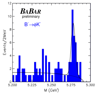
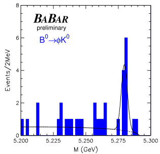
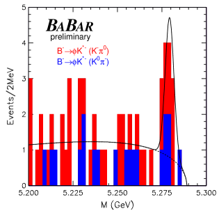
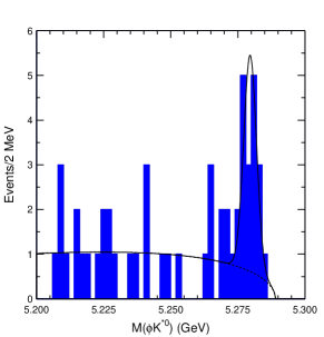
Figure 16: The $m_{\rm ES}$ distribution for a) $B^{\pm}\rightarrow\phi K^{\pm}$, b) $B^{0}\rightarrow\phi K^{0}_{\scriptscriptstyle S}$, and c) $B^{\pm}\rightarrow\phi K^{*\pm}$, and d) $B^{0}\rightarrow\phi K^{*0}$. Discrete cuts have been applied to enhance the signal to background rate for each decay mode.

time dependent asymmetry in the decay $B^{0}\rightarrow\phi K^{0}_{\scriptscriptstyle S}$ will allow an interesting comparison, especially sensitive to new physics, with the $\sin\!2\beta$ measurement in $B^{0}\rightarrow{J\mskip-3.0mu/\mskip-2.0mu\psi\mskip 2.0mu}K^{0}_{\scriptscriptstyle S}$.

5 Future prospects for BABAR

The first year and half of BABAR data has yielded a number of important results, with the observation of CP violation the most notable. The future for BABAR looks equally bright; a data sample of order $500\mbox{\,fb}^{-1}$ is expected to be accumulated in the next few years. This size data sample will enable significant improvements in accuracy for $\sin\!2\beta$, an accurate measurement of $\sin\!2\alpha_{\rm Eff}$, and measurements of the third CP angle $\gamma$.

6 Acknowledgments

We are grateful for the extraordinary contributions of our PEP-II colleagues for the superb operation of the B factory. This work is supported by Department of Energy contract DE-AC03-76SF00515.

7 References

References

- [1] L. Wolfenstein, Phys. Rev. Lett. 51, 1945 (1983).
- [2] Lee, S.Y. Accelerator Physics (World Scientific, Singapore, 1999).
- [3] L. Hendrickson et al., “Slow feedback systems for PEP-II”, Presented at 7th European Particle Accelerator Conferences (EPAC 2000), Vienna, Austria, 26-30 Jun 2000 SLAC-PUB-8480.
- [4] T. Himel, Ann. Rev. Nucl. Part. Sci. 47, 157 (1997).
- [5] B. Aubert et al. [BABAR Collaboration], The BaBar detector, arXiv:hep-ex/0105044.
- [6] B. Aubert et al. [BABAR Collaboration], Phys. Rev. Lett. 87, 091801 (2001).
- [7] B. Aubert et al. [BABAR Collaboration], Phys. Rev. Lett. 87, 201803 (2001).
- [8] B. Aubert et al. [BABAR Collaboration], arXiv:hep-ex/0107036.
- [9] B. Aubert et al. [BABAR Collaboration], arXiv:hep-ex/0110065.
- [10] B. Aubert et al. [BABAR Collaboration], Phys. Rev. Lett. 87, 151802 (2001).
- [11] B. Aubert et al. [BABAR Collaboration], Phys. Rev. Lett. 87, 151801 (2001).