Tests of hard and soft QCD with $\mathrm{e^{+}e^{-}}$ Annihilation Data

Abstract

Experimental tests of QCD predictions for event shape distributions combining contributions from hard and soft processes are discussed. The hard processes are predicted by perturbative QCD calculations. The soft processes cannot be calculated directly using perturbative QCD, they are treated by a power correction model based on the analysis of infrared renormalons. Furthermore, an analysis of the gauge structure of QCD is presented using fits of the colour factors within the same combined QCD predictions.

1 INTRODUCTION

Hadron production in $\mathrm{e^{+}e^{-}}$ annihilation is a well-suited process for the study of the interplay between hard and soft QCD. The lack of interference with the initial state improves the understanding of the hadronic final state in terms of QCD. The availability of data sets at many energy points with centre of mass (cms) energies $\sqrt{s}$ between 14 and 209 GeV allows to separate the hard and soft contributions.

The hard QCD processes, i.e. the radiation of gluons from the quarks produced at the electroweak vertex and subsequent higher order processes are well understood in perturbative QCD (pQCD) [1]. The production of multi-jet events is clear evidence for the existence of gluons and is successfully described by pQCD.

The soft contributions to hadron production in $\mathrm{e^{+}e^{-}}$ annihilation are connected with the transition from the partons (quarks and gluons) generated by hard processes to the hadrons observed in the experiment. This transition is referred to as hadronisation and takes place at energy scales of approximately a light hadron mass, i.e. ${\cal O}(100)$ MeV, where pQCD calculations are not reliable due to the rapid growth of the strong coupling $\alpha_{\mathrm{S}}$. The soft contributions are known to scale like an inverse power of the cms energy; for most observables the scaling is $1/\sqrt{s}$.

2 POWER CORRECTIONS AND INFRARED RENORMALONS

At energy scales $Q=\Lambda_{\mathrm{QCD}}$ perturbative evolution of $\alpha_{\mathrm{S}}(Q)$ breaks down completely due to the Landau pole at $\Lambda_{\mathrm{QCD}}$. It is therefore impossible to attempt pQCD calculations of soft processes without further assumptions.

In order to clarify which assumptions are needed a phenomenological model of hadronisation is considered. The longitudinal phase space model or tube model goes back to Feynman [2]. One considers a $\mathrm{q\overline{q}}$ system produced e.g. in $\mathrm{e^{+}e^{-}}$ annihilation in the cms system. The two primary partons move apart with velocity $v/c\simeq 1$. In such a situation the production of soft gluons will be approximately independent of their (pseudo-) rapidity $\eta^{\prime}=-\log(\tan(\Theta_{i}/2))$, see figure 1.

Figure 1: Sketch of a $\mathrm{q\overline{q}}$ system in $\eta^{\prime}-k_{\mathrm{t}}$ space.

The change to e.g. the observable Thrust $1-T$ due to the production of a soft gluon at angle $\Theta_{i}$ with transverse momentum $k_{\mathrm{t},i}$ is $\Delta(1-T)_{i}\simeq k_{\mathrm{t},i}/Qe^{-|\eta^{\prime}_{i}|}$. This observation is generalised to write the soft or non-perturbative contribution to the mean value of the $1-T$ distribution as follows:

$$\mbox{$\langle 1-T\rangle$}_{\mathrm{NP}}=\int\frac{k_{\mathrm{t}}}{Q}\Phi(k_{\mathrm{t}})\frac{\mathrm{d}k_{\mathrm{t}}}{k_{\mathrm{t}}}\cdot\int e^{-|\eta^{\prime}|}d\eta^{\prime}$$ (1)

The function $\Phi(k_{\mathrm{t}})\sim\alpha_{\mathrm{S}}(k_{\mathrm{t}})$ is the distribution of soft particles in $k_{\mathrm{t}}$. The first integral in equation (1) is summarised as $\alpha_{0}/Q$ independent of the observable and the second as a constant $c_{1-T}$ dependent on the observable. The quantity $\alpha_{0}\sim\int\alpha_{\mathrm{S}}(k_{\mathrm{t}})\mathrm{d}k_{\mathrm{t}}$ can only exist when $\alpha_{\mathrm{S}}(k_{\mathrm{t}})$ is identified with a non-perturbative strong coupling $\alpha_{\mathrm{S}}^{\mathrm{NP}}(k_{\mathrm{t}})$ which is assumed to be finite at low $k_{\mathrm{t}}$ around and below the Landau pole.

A more formal approach to the origin of soft contributions is the study of infrared renormalons, i.e. the divergence of asymptotic pQCD predictions due to the integration of low momenta in quark loops in gluon lines [3]. The infrared renormalon divergence of the $\mathcal{O}(\alpha_{\mathrm{S}}^{n})$ term in a pQCD prediction is factorial in $n$: $r_{n}\alpha_{S}^{n+1}\sim(2\beta_{0}/p)^{n}n!\alpha_{S}^{n+1}$. With Sterlings formula to replace $n!$ one finds $r_{n}\alpha_{S}^{n+1}\sim(2\beta_{0}\alpha_{\mathrm{S}}/p)^{n}n^{n}e^{-n}\alpha_{\mathrm{S}}$. The convergence of the series is optimal for $n=p/(2\beta_{0}\alpha_{\mathrm{S}})$. Based on this relation one finds

$$r_{n}\alpha_{S}^{n+1}\sim\left(\frac{\Lambda_{\mathrm{QCD}}}{Q}\right)^{p}$$ (2)

where the first order relation between $\alpha_{\mathrm{S}}$ and $\Lambda_{\mathrm{QCD}}$ has been used. The result shows that infrared renormalon contributions to pQCD predictions scale like $Q^{-p}$ similar to the soft contribution studied in the tube model, see equation (1).

The power correction model of Dokshitzer, Marchesini and Webber (DMW) extracts the structure of power correction terms from analysis of infrared renormalon contributions [4]. The model assumes that a non-perturbative strong coupling exists around and below the Landau pole and that the quantity $\alpha_{0}(\mu_{\mathrm{I}})=1/\mu_{\mathrm{I}}\int_{0}^{\mu_{\mathrm{I}}}\alpha_{\mathrm{S}}^{\mathrm{NP}}(k_{\mathrm{t}})\mathrm{d}k_{\mathrm{t}}$ can be defined. The value of $\mu_{\mathrm{I}}$ is chosen to be safely within the perturbative region, usually $\mu_{\mathrm{I}}=2$ GeV.

The main result for the effects of power corrections on distributions $F(y)$ of the event shape observables $1-T$, $M_{\mathrm{H}}$ and $C$ is that the perturbative prediction $F_{\mathrm{PT}}(y)$ is shifted [5, 6, 7]:

$$F(y)=F_{\mathrm{PT}}(y-c_{\mathrm{y}}P)$$ (3)

where $c_{\mathrm{y}}$ is an observable dependent constant and $P\sim M\mu_{\mathrm{I}}/Q(\alpha_{0}(\mu_{\mathrm{I}})-\alpha_{\mathrm{S}})$ is universal, i.e. independent of the observable [6]. The factor $P$ contains the $1/Q$ scaling and the so-called Milan-factor $M$ which takes two-loop effects into account. The non-perturbative parameter $\alpha_{0}$ is explicitly matched with the perturbative strong coupling $\alpha_{\mathrm{S}}$. For the event shape observables $B_{\mathrm{T}}$ and $B_{\mathrm{W}}$ the predictions are more involved and the shape of the pQCD prediction is modified in addition to the shift [7]. For mean values of $1-T$, $M_{\mathrm{H}}$ and $C$ the prediction is:

$$\mbox{$\langle y\rangle$}=\mbox{$\langle y\rangle$}_{\mathrm{PT}}+c_{\mathrm{y}}P$$ (4)

For $\langle B_{\mathrm{T}}\rangle$ and $\langle B_{\mathrm{W}}\rangle$ the predictions are also more involved.

3 EXPERIMENTAL TESTS

Distributions and mean values of event shape observables measured in $\mathrm{e^{+}e^{-}}$ annihilation at many cms energy points between 14 and more than 200 GeV have been used recently by several groups to study power corrections [8, 9, 10, 11]. This report will present mainly results from [8]. In all of these studies pQCD predictions in $\mathcal{O}(\alpha_{\mathrm{S}}^{2})$+NLLA [12, 13, 14] are used for event shape distributions while $\mathcal{O}(\alpha_{\mathrm{S}}^{2})$ [15] predictions are employed for mean values. The pQCD predictions are added together with the power correction predictions. The resulting expressions are functions of the strong coupling $\alpha_{\mathrm{S}}(M_{\mathrm{Z}})$ and of the non-perturbative parameter $\alpha_{0}$. The complete predictions are compared with data for event shape distributions or mean values as published by the experiments.

Figure 2: Scaled distributions of $1-T$. The solid lines show the result of the fit of the combined pQCD and power correction prediction. The dotted lines represent an extrapolation of the result [8].

Figure 2 shows the results fitting the data for $1-T$ distributions measured at cms energies from 14 to 189 GeV. The data from experiments at $\sqrt{s}<M_{\mathrm{Z}}$ are corrected for the effects of $\mathrm{e^{+}e^{-}}\rightarrow\mathrm{b\overline{b}}$ events [8]. The data in the fitted regions are well reproduced by the theory (solid lines). The dotted lines present extrapolations outside of the fitted regions using the fit results for $\alpha_{\mathrm{S}}(M_{\mathrm{Z}})$ and $\alpha_{0}$ which describe the data reasonably well. The agreement between theory and experiment is similar for the other observables.

Figure 3: The cms energy dependence of $\langle 1-T\rangle$ is shown. The solid lines show the result of the fit of combined $\mathcal{O}(\alpha_{\mathrm{S}}^{2})$ QCD calculations with power corrections while the dashed lines indicate the perturbative contribution [8].

Figure 3 (solid line) presents the result of a fit to measurements of $\langle M_{\mathrm{H}}^{2}\rangle$ at $\sqrt{s}=14$ to 189 GeV. The data are well described by the fitted theory. The dotted line in figure 3 shows the perturbative part of the prediction; one observes that the soft (power correction) contributions increase at low $\sqrt{s}$.

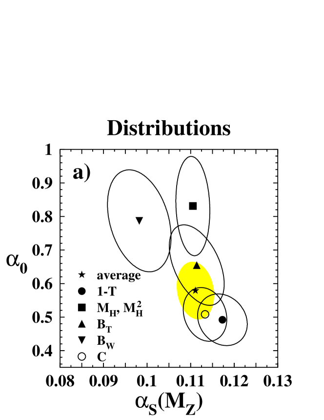
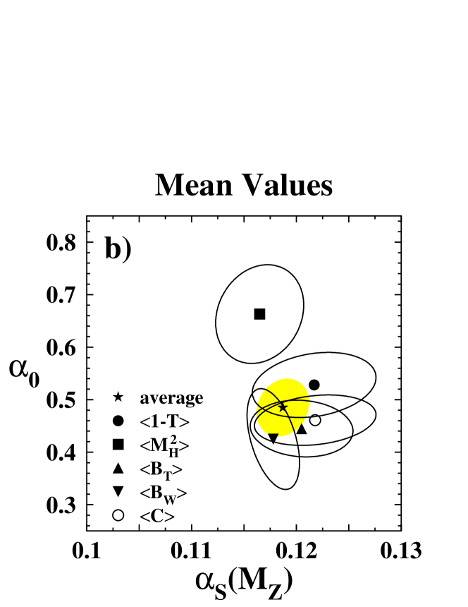
Figure 4: Results for $\alpha_{\mathrm{S}}(M_{\mathrm{Z}})$ and $\alpha_{0}(2~{}\mathrm{GeV})$ for distributions (top) and mean values (bottom). The error ellipses show one standard deviation uncertainties (38% CL) [8].

The combined results from the analysis of distributions are $\alpha_{\mathrm{S}}(M_{\mathrm{Z}})=0.1111^{+0.0048}_{-0.0037}$ and $\alpha_{0}(2~{}\mathrm{GeV})=0.579^{+0.100}_{-0.072}$. The relatively small value of $\alpha_{\mathrm{S}}(M_{\mathrm{Z}})$ compared e.g. to the world average $\alpha_{\mathrm{S}}(M_{\mathrm{Z}})=0.1184\pm 0.0034$ [16] is due to small results from $M_{\mathrm{H}}$ and $B_{\mathrm{W}}$. The individual and the combined results are shown as points with one-standard-deviation error ellipses in figure 4 a).

From the analysis of mean values the combined results are $\alpha_{\mathrm{S}}(M_{\mathrm{Z}})=0.1187^{+0.0031}_{-0.0020}$ and $\alpha_{0}(2~{}\mathrm{GeV})=0.485^{+0.066}_{-0.045}$ in reasonable agreement with the results from distributions. Figure 4 b) presents the individual and combined results from fits to mean values as points with one-standard-deviation error ellipses. Combining both analyses yields the final results: $\alpha_{\mathrm{S}}(M_{\mathrm{Z}})=0.1171^{+0.0032}_{-0.0020}$ and $\alpha_{0}(2~{}\mathrm{GeV})=0.513^{+0.066}_{-0.045}$ .

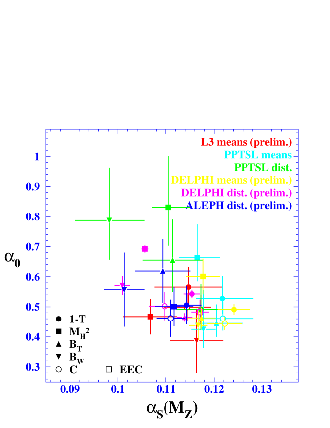
Figure 5: The figure shows a summary of results for $\alpha_{\mathrm{S}}(M_{\mathrm{Z}})$ and $\alpha_{0}(2~{}\mathrm{GeV})$ from power correction studies [8, 9, 10, 11]. The results labelled PPTSL are from [8].

Figure 5 shows a summary of results for $\alpha_{\mathrm{S}}(M_{\mathrm{Z}})$ and $\alpha_{0}(2~{}\mathrm{GeV})$ obtained in comparable analyses by several groups [8, 9, 10, 11]. One observes reasonable agreement between the individual measurements. The comparable results for $M_{\mathrm{H}}$ and $B_{\mathrm{W}}$ from [8] and [10] differ, because in [10] hadron mass effects on power corrections are considered [2]. The non-perturbative parameter $\alpha_{0}$ appears universal within about 20% as expected [6] while the values for $\alpha_{\mathrm{S}}(M_{\mathrm{Z}})$ are compatible with the world average [16].

4 QCD COLOUR FACTORS

The analysis of event shape distributions described above can be generalised to study the gauge structure of QCD [17]. The $\mathcal{O}(\alpha_{\mathrm{S}}^{2})$+NLLA pQCD predictions can be decomposed into additive terms which are proportional to products of the QCD colour factors. This analysis constitutes an experimental test of the gauge symmetry of QCD via radiative corrections. The values of the colour factors correspond to the relative size of contributions from three fundamental processes i) gluon radiation from a quark ($C_{\mathrm{F}}$), ii) conversion of a gluon in a $\mathrm{q\overline{q}}$ pair ($T_{\mathrm{F}}$$n_{\mathrm{f}}$) and iii) radiation of a gluon from a gluon (triple gluon vertex TGV) ($C_{\mathrm{A}}$). Higher order processes like the quartic gluon vertex are not accessible with the available pQCD calculations.

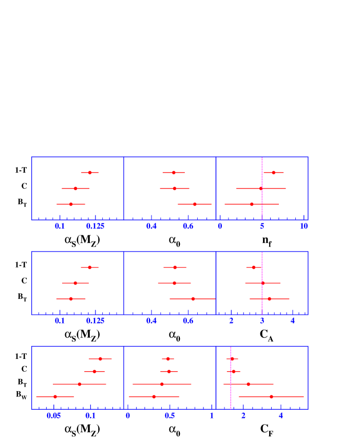
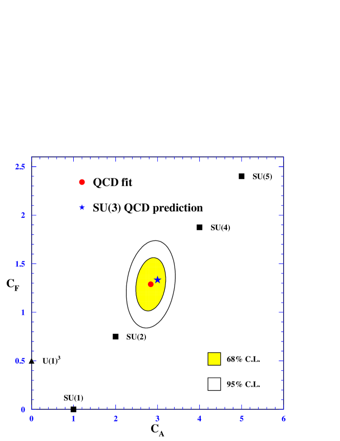
Figure 6: The figure at the top shows results for $\alpha_{\mathrm{S}}(M_{\mathrm{Z}})$, $\alpha_{0}(2~{}\mathrm{GeV})$ and one of the colour factors for individual observables as indicated. The error bars show total uncertainties and the dotted lines show the expectation from SU(3) QCD. The figure at the bottom presents combined results for $C_{\mathrm{A}}$ and $C_{\mathrm{F}}$ from fits to $\alpha_{\mathrm{S}}(M_{\mathrm{Z}})$, $C_{\mathrm{A}}$ and $C_{\mathrm{F}}$ with $1-T$ and $C$. The square and triangle symbols indicate expectations for $C_{\mathrm{A}}$ and $C_{\mathrm{F}}$ for several symmetry groups [17].

The values of the colour factors are determined in the theory when a particular gauge symmetry group is chosen under which the Lagrangian of theory must be locally invariant. The local gauge symmetry for QCD is SU(3) with $C_{\mathrm{F}}=4/3$, $C_{\mathrm{A}}=3$ and $T_{\mathrm{F}}=1/2$. The number of active quark flavours is $n_{\mathrm{f}}=5$ at the cms energies of the currently available data. The perturbative evolution (running) of the strong coupling is also sensitive to the colour factors since quark loops and gluon loops have the opposite effect. In $\mathcal{O}(\alpha_{\mathrm{S}})$ the evolution of the strong coupling between two scales $Q$ and $\mu$ is given by $\alpha_{\mathrm{S}}(Q)=\alpha_{\mathrm{S}}(\mu)/(1+2\beta_{0}\alpha_{\mathrm{S}}(\mu)\ln(Q/\mu))$ with $\beta_{0}=(11C_{\mathrm{A}}-2n_{\mathrm{f}})/(12\pi)$.

The power correction calculations are also functions of the QCD colour factors. In the analysis the colour factors in the pQCD predictions as well as in the power corrections are considered as additional free parameters to be determined from the data. In this way the dependence on the hadronisation model is reduced compared to traditional analyses relying on Monte Carlo models of hadronisation, because in the Monte Carlo models the colour factors are fixed [18, 19, 20].

Figure 6 (top) shows the results of simultaneous fits of $\alpha_{\mathrm{S}}(M_{\mathrm{Z}})$, $\alpha_{0}(2~{}\mathrm{GeV})$ and one colour factor where the other colour factors have been kept fixed at their SU(3) values. The fits are stable with the observables $1-T$ and $C$. Some fits are not stable with the observables $B_{\mathrm{T}}$ and $B_{\mathrm{W}}$. In alternative fits the non-perturbative parameter $\alpha_{0}$ was kept fixed at a previously measured value and is varied by its total error as a systematic uncertainty. The results and the uncertainties are consistent between the two types of fit. The variation of $\alpha_{0}$ in the fits avoids a possible bias which might be present when $\alpha_{0}$ is fixed to a value measured with colour factors fixed to their standard values. Combined results for the colour factors measured individually are $n_{\mathrm{f}}=5.64\pm 1.35$, $C_{\mathrm{A}}=2.88\pm 0.27$ and $C_{\mathrm{F}}=1.45\pm 0.27$. The corresponding results for $\alpha_{\mathrm{S}}(M_{\mathrm{Z}})$ and $\alpha_{0}$ are consistent with previous measurements.

Figure 6 (bottom) presents the combined results of simultaneous fits to $1-T$ and $C$ of $\alpha_{\mathrm{S}}(M_{\mathrm{Z}})$, $C_{\mathrm{A}}$ and $C_{\mathrm{F}}$ with $\alpha_{0}$ fixed to previously measured value. Such fits with $\alpha_{0}$ as a free parameter turn out to be unstable mainly due to limited precision of the data. The results are $C_{\mathrm{A}}=2.84\pm 0.24$ and $C_{\mathrm{F}}=1.29\pm 0.18$ with a consistent value of $\alpha_{\mathrm{S}}(M_{\mathrm{Z}})=0.119\pm 0.010$ and consistent with the expectation from SU(3). Several other possible gauge groups are excluded.

5 SUMMARY

The analyses of power corrections discussed in section 3 show that it is possible to describe event shape distributions and mean values in $\mathrm{e^{+}e^{-}}$ annihilation data with combined pQCD and power correction predictions without the need for Monte Carlo based hadronisation corrections. Global fits of the combined theory with only $\alpha_{\mathrm{S}}(M_{\mathrm{Z}})$ and $\alpha_{0}(2~{}\mathrm{GeV})$ as free parameters to event shape data measured at $\sqrt{s}=14$ GeV up to the highest LEP 2 energies lead to a satisfactory agreement with the data. The non-perturbative parameter $\alpha_{0}(2~{}\mathrm{GeV})$ is found to be universal, i.e. independent of the observable, within the expected theoretical uncertainty of about 20%.

A generalisation of the power correction analysis to also vary the QCD colour factors provides a measurement of the colour factors based on the QCD radiative corrections in the pQCD and the power correction predictions. The results for the colour factors are consistent with the expectations from SU(3) as the gauge group of QCD while the total uncertainties are competitive with analyses of angular correlations in 4-jet final states in $\mathrm{e^{+}e^{-}}$ annihilation.

One of the legacies of LEP, SLC and their predecessors TRISTAN, PETRA and PEP is the wealth of measurements using hadronic final states in $\mathrm{e^{+}e^{-}}$ annihilation. These data made is possible to test and verify combined predictions for hard (pQCD) and soft (power corrections) processes. Based on these tests our understanding of the hard and soft processes and their interplay has improved significantly.

The author would like to take the opportunity to thank the organisers for a stimulating and entertaining meeting.

References

- [1] R.K. Ellis, W.J. Stirling, B.R. Webber: QCD and Collider Physics. Vol. 8 of Cambridge Monographs on Particle Physics, Nuclear Physics and Cosmology, Cambridge University Press (1996)
- [2] G.P. Salam, D. Wicke: JHEP 05 (2001) 061
- [3] M. Beneke, V.M. Braun: In: At the Frontier of Particle Physics/Handbook of QCD, Vol. 3, 1719, World Scientific (2001)
- [4] Yu.L. Dokshitzer, G. Marchesini, B.R. Webber: Nucl. Phys. B 469 (1996) 93
- [5] Yu.L. Dokshitzer, B.R. Webber: Phys. Lett. B 404 (1997) 321
- [6] Yu.L. Dokshitzer, A. Lucenti, G. Marchesini, G.P. Salam: J. High Energy Phys. 5 (1998) 003
- [7] Yu.L. Dokshitzer, G. Marchesini, G.P. Salam: Eur. Phys. J. direct C 3 (1999) 1
- [8] P.A. Movilla Fernández, S. Bethke, O. Biebel, S. Kluth: Eur. Phys. J. C (2001) DOI 10.1007/s100520100750
- [9] L3 Coll., M. Acciarri et al.: L3 note 2555 (2000), Submitted to XXXth International Conference on High Energy Physics, July 27 - August 2, Osaka, Japan
- [10] DELPHI Coll., P. Abreu et al.: DELPHI 2001-062 CONF 490 (2001), Submitted to International Europhysics Conference on High Energy Physics, July 12-18, 2001, Budapest, Hungary
- [11] ALEPH Coll., D. Abbaneo et al.: ALEPH 2000-044 (2000), Submitted to XXXth International Conference on High Energy Physics, July 27 - August 2, Osaka, Japan
- [12] S. Catani, L. Trentadue, G. Turnock, B.R. Webber: Nucl. Phys. B 407 (1993) 3
- [13] Yu.L. Dokshitzer, A. Lucenti, G. Marchesini, G.P. Salam: J. High Energy Phys. 1 (1998) 011
- [14] S. Catani, B.R. Webber: Phys. Lett. B 427 (1998) 377
- [15] Z. Kunszt, P. Nason: In: Z physics at LEP 1, G. Altarelli, R. Kleiss, C. Verzegnassi (eds.), Vol. 1, CERN 89-08 (1989)
- [16] S. Bethke: J. Phys. G 26 (2000) R27
- [17] S. Kluth et al.: Eur. Phys. J. C 21 (2001) 199
- [18] ALEPH Coll., R. Barate et al.: Z. Phys. C 76 (1997) 1
- [19] DELPHI Coll., P. Abreu et al.: Phys. Lett. B 414 (1997) 401
- [20] OPAL Coll., G. Abbiendi et al.: Eur. Phys. J. C 20 (2001) 601