DELPHI Collaboration              DELPHI 99-150 RICH 95 03 October, 1999

MACRIB
High efficiency - high purity
hadron identification for DELPHI
Z. Albrecht, M. Feindt and M. Moch
Institut für Experimentelle Kernphysik
Universität Karlsruhe

Analysis of the data shows that hadron tags of the two standard DELPHI particle identification packages RIBMEAN and HADSIGN are weakly correlated. This led to the idea of constructing a neural network for both kaon and proton identification using as input the existing tags from RIBMEAN and HADSIGN, as well as preproccessed TPC and RICH detector measurements together with additional dE/dx information from the DELPHI vertex detector. It will be shown in this note that the net output is much more efficient at the same purity than the HADSIGN or RIBMEAN tags alone. We present an easy-to-use routine performing the necessary calculations.

1 Introduction

With the Rich Imaging Cherenkov Chamber (RICH) DELPHI possesses a unique and very important hadron identification tool. The two informations from the liquid and gas radiators can be combined with the dE/dx information measured in the Time Projection Chamber (TPC) [1] to achieve separation of hadron species at different momenta (fig. 1).

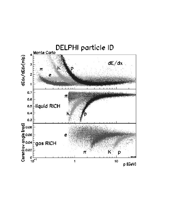
Figure 1: DELPHI particle identification

In different momentum ranges the single detectors (TPC, RICH) can distinguish the hadrons in different ways and quality. The description of the particle identification algorithms for the Rich detectors based on RIBMEAN[2]. On first sight, there is no problem if the bands of the single hadrons can be well separated. An obvious problem is how to deal with momentum ranges where one detector cannot separate between different particle hypotheses and another detector is in the so-called veto mode i.e. when one expects no signal for a track in the detector. This happens e.g. in the range $5~{}\textrm{GeV}<p<10~{}\textrm{GeV}$ for kaons and protons. This is handled in HADSIGN and RIBMEAN in different ways [3, 4]. Veto signals are especially hard to establish in the case of background due to large particle density (in case of RIBMEAN see [5]). Especially the background photon handling is done differently in HADSIGN and RIBMEAN. We later show that even in the case where two bands are clearly separated a problem appears in at least RIBMEAN. We do not have intermediate information to check HADSIGN at the SDST level. From the above considerations it is clear that the construction of simple tags is strongly momentum dependent and not a trivial task.

As one can see in figure 1, below 0.7 GeV no RICH information is available. In addition, 21% of the tracks have less then 30 TPC wire hits, so that in these cases no particle identification is possible with the TPC as the only detector. As in the case of higher momentum particles, i.e. above 0.7 GeV, an independent measurement would contribute a large boost to the efficiency of hadron tagging. This is supplied by the Vertex Detector, usually used for spatial measurements only, but the signal in the silicon tracker also gives signal height information proportional to the deposited energy lost by the passing particle. The signals from the different hypothesis can be seen in figure 2.

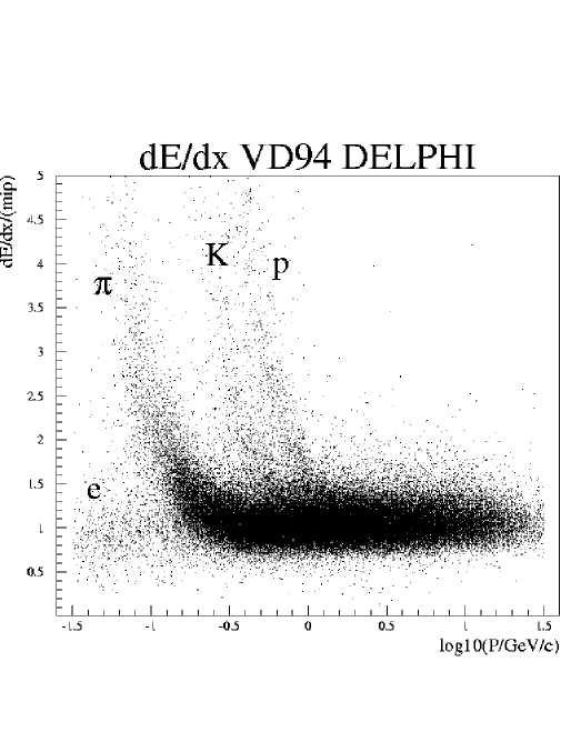
Figure 2: The vertex detector dE/dx with three hits and more for the whole momentum range, measured with the 94 vertex detector. Clearly visible are the e, $\pi$, Kaon and proton bands.

In this note we present the MACRIB package which combines the benefits of both RICH algorithms and dE/dx information for the high momentum region. For the low momentum region the combined dE/dx information of both the TPC and the VD are used. The combination is done using a neural network, which has a much better performance than any of it’s input variables alone.

2 Comparison of HADSIGN and RIBMEAN

RIBMEAN provides a tag between -1 and 3 according to the probability for a given particle calculated within the routine. -1 means that no information is available, 0 stands for sure background and 1,2,3 for the loose, standard and tight kaon tags. In addition to RIBMEAN, HADSIGN introduces a very tight kaon tag with code 4 and a very loose tag with code 0.5. For the case of no information and no identification both algorithms give -1 and 0 respectively. In the ideal case both approaches should give the same or at least similar tags for a particle. A comparison of the tags shows that they are hardly correlated (see fig 3). There are situations where RIBMEAN works more efficiently and vice versa. A possible reason for this discrepancy is the different approach for the ring finding algorithm in the RICH detectors. RIBMEAN divides the plane around a track intersection point into rings with different radii according to each particle hypothesis ($e,\ \mu,\ \pi,K$ and $p$). The photoelectrons are weighted within the rings. Different weights are given depending on the background environment, e.g. on the (non-)ambiguity and the geometrical position in the ring. The cluster with the largest sum of weights is selected. For isolated tracks this algorithm gives a very reliable result. For high density tracks the rings overlap and not all ambiguities can be solved. In these cases the performance of this method drops.

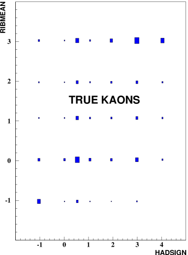
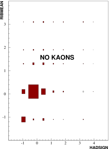
Figure 3: Comparison of combined the HADSIGN and RIBMEAN kaon tags shows the anticorrelation in the tagging of the same particle as a tight kaon through one routine and as a non-kaon through the other.

In contrast, HADSIGN treats background by including it in the model. It sums up the photo-electrons as a function of the distance from the intersection point, regardless of its origin. Next a maximum likelihood technique is applied to the obtained distribution. According to the result of the fit HADSIGN assigns a probability to the different hypotheses. In this way, the performance of HADSIGN is relatively independent of background.

3 A neural network approach

This observation was the motivation for optimally combining both algorithms using a simple feed forward network with backpropagation. A schematic example of the topology of this kind of network is given in figure 4. Three sets of neural networks have been constructed for kaon and proton identification:

• $p>0.7$ GeV with full RICH information,

• $p>0.7$ GeV with no liquid RICH information,

• $p\leq 0.7$ GeV TPC dE/dx combined with dE/dx measurements of the vertex detector.

The distinction between the cases with and without liquid information is necessary for the Monte Carlo Data agreement was not satisfactory. The reason originates from the fact that there are periods in the data where the RICH is only partly functional. For the case of no liquid RICH information present, a new network is required due to the relatively large number of input nodes requiring liquid information and to the lack of non-liquid radiator information in the 1994 Monte Carlo simulation for the training. For the training of events with only gas information a MC sample from 1993 has been used.

Figure 4: An example for a simple feed forward neural network with three layers.

3.1 Input variables for the nets with liquid RICH information

The networks have four layers, 16 input nodes, one bias node, 19 nodes in the hidden layer and one output node. Several variables of the RICH and the TPC are used as input variables, as detailed below. Many of the variables have been optimised for the use as a neural network input. For the training we used 800,000 kaons and approximately the same number of non-kaons from the 94C2 $Z^{0}\to q\bar{q}$ Monte Carlo datasets. We use the following variables as input for the kaon net:

1. the RIBMEAN RICH kaon tag. The order of codes 0 and -1 has been interchanged in order to make the kaon probability a monotonically rising function of the tag.

2. the HADSIGN RICH kaon tag. The order of codes 0 and -1 has been interchanged in order to make the kaon probability a monotonically rising function of the tag.

3. the dE/dx kaon tag from HADSIGN. The order of codes 0 and -1 has been interchanged in order to make the kaon probability a monotonically rising function of the tag.

4. the logarithm of the ratio of the gas RICH probabilities of the kaon hypothesis to the pion hypothesis for kaon separation from pions with gas RICH. If no gas measurement is available, the value is set to 0.

5. the logarithm of the ratio of the liquid RICH probabilities of the kaon hypothesis to the pion hypothesis for kaon separation from pions with liquid RICH. If no liquid measurement is available, the value is set to 0.

6. the electron neural net output from ELEPHANT, to suppress electrons faking kaons.

7. the combined HADSIGN proton tag, to suppress protons faking kaons. The order of codes 0 and -1 has been interchanged in order to make the proton probability a monotonically rising function of the tag.

8. the logarithm of the ratio of the dE/dx probabilities of the kaon hypothesis to the pion hypothesis for kaon separation from pions with dE/dx. If no dE/dx measurement is available, the value is set to 0.

9. the logarithm of the likelihood ratio for the number of photons in the liquid RICH for the kaon and pion hypotheses. This is computed in the following way: The number of reconstructed photons in the liquid radiator is subtracted from the expected number of photons for the pion hypothesis as a function of the expectation and the particle hypothesis, in 7 expectation bins from 5 to 20 photons. In each of the bins the normalised Monte Carlo distribution is fitted to a double Gaussian. The variation of the 6 fit parameters in the 7 expectation bins is then parametrised, such that the probability density is available as a continuous function of expectation and particle hypothesis. The input variable is the logarithm of the ratio of these functions for kaon and pion hypotheses.

   

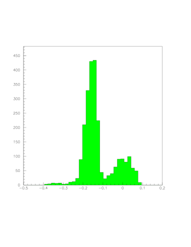
   Figure 5: Performance of the liquid RICH data on the Čerenkov angle. The plot shows the difference between measured and expected angle for the pion hypothesis for true kaons in the momentum region 0.7-0.9 GeV, i.e. in a region where the kaon band is significantly separated from the pion band. The distribution around -0.16 shows correctly identified kaons, whereas the peak at 0. shows misidentified kaons.

10. the logarithm of the likelihood ratio for the number of photons in the liquid RICH for the kaon and proton hypotheses to suppress proton contamination.

11. the logarithm of the likelihood ratio for the number of photons in the gas RICH for the kaon and pion hypotheses in the kaon gas band region.

12. the logarithm of the likelihood ratio for kaon and pion hypotheses in the kaon gas veto region. This is computed in the following way: In the momentum region where one expects to see a ring for pions, but not for kaons, we distinguish the following cases:

    • no photon is observed (i.e. a good veto): as a function of the expected number of photons for the pion hypothesis, and separately for tracks including the Outer Detector (signalling a more reliable track interpolation in the RICH) the ratio of real kaons to all tracks as expected is parametrised.

    • one photon is observed (i.e. a slightly worse veto): this one photon could be real or background, thus the separation is worse in this case. The same procedure as above is performed.

    • more than one photon is observed, and an angle measurement performed (i.e. a bad or no veto): Even in this case one can distinguish how often such an assignment is wrong. Both the angle and the number of photon measurements should be compatible with the pion hypothesis.

    Outside the interesting momentum region the variable is set to 0.5.

13. the information if the OD was used in the track reconstruction.

14. the muon tag for the kaon separation from muons.

15. the momentum of the particle

    

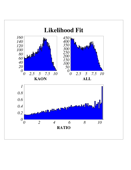
    Figure 6: In the momentum region where one expects to see a ring for pions, but not for kaons for the case when no or only one photon is observed the following likelihood fit is made. As a function of the expected number of photons for the pion hypothesis the ratio of real kaons to all tracks as expected is parametrised.

16. the logarithm of the likelihood ratio for the Čerenkov angle measurement in the gas RICH for the kaon and pion hypotheses in the kaon gas band region.

17. the logarithm of the likelihood ratio for the Čerenkov angle measurement in the liquid RICH for the kaon and pion hypotheses in the kaon liquid band region below 4 GeV. Outside this region the variable is set to 0.5, outside the usual region on the background side.

18. the probability of the dE/dx pull of the kaon hypothesis.

In order to reduce the number of input variables, two pairs of RICH measurements were put together to form one without losing information, since the momentum regions of the pairs do not interfere. These are the likelihood ratios for the number of photons in the liquid and gas radiators and the likelihood ratios for the Cerenkov angle measurement for the liquid and gas.

For the proton network an analogous set of input variables were used and for the training $\approx$250,000 protons were used mixed with the same amount of background. Additionally a pion veto region is introduced for the liquid radiator in the momentum region between $0.7~{}\text{GeV}<p<1.2~{}\text{GeV}$. The information is treated in a similar way as is done for the kaons in the gas veto region.

3.2 Net input variables without liquid RICH information

The kaon network has three layers, 16 input nodes, one bias node, 17 nodes in the hidden layer and one output node. RICH gas and TPC variables are used as input variables. For the training we used the 93D2 $q\bar{q}$ simulation with a sample of 130,000 kaons and approximately the same number of non-kaons. We use the following variables as input for the kaon net (for the detailed description of the variables see section before):

1. the RIBMEAN RICH kaon tag.

2. the HADSIGN RICH kaon tag.

3. the HADSIGN combined proton tag

4. the dE/dx kaon tag from HADSIGN.

5. $\log(\frac{P_{K}}{P_{\pi}})$ from the TPC dE/dx measurement

6. Prob(Kaon Pull) from the TPC.

7. Prob(Pion Pull) from the TPC.

8. $\log(\frac{P_{K}}{P_{\pi}})$ from the gas RICH

9. $\log\text{-likelihood}\left(\frac{N\gamma_{K}}{N\gamma_{\pi}}\right)$ in the kaon gas band region.

10. $\log\text{-likelihood}\left(\frac{\Theta_{K}}{\Theta_{\pi}}\right)$ in the kaon gas band region.

11. for $0~{}\text{or}~{}1\gamma:\frac{K}{all}(N\gamma_{\pi,expected})$ or
    for $\geq 2\gamma:\text{Prob}(\Theta_{\pi},N\gamma_{\pi})$ with 2 degrees of freedom in the kaon gas veto region.

12. the logarithm of the ratio of the dE/dx probabilities of the kaon hypothesis to the pion hypothesis for kaon separation from pions with the vertex detector.

13. the logarithm of the ratio of the dE/dx probabilities of the proton hypothesis to the pion hypothesis for heavy particle separation from pions with the vertex detector.

14. the electron neural network output

15. the muon tag

16. the OD flag

17. the momentum of the particle

To partially compensate the loss of the liquid radiator information in the momentum region of $0.7~{}\text{Gev}<p<2.5~{}\text{Gev}$, the vertex detector measurement was introduced into the net. The separation performance of the VD dE/dx in this region is not as good as of the liquid RICH but it helps to solve some ambiguities. For the proton network $\approx$50,000 protons were used mixed with the same amount of background and all kaon inputs were changed to proton variables. The proton net has 15 input nodes and one bias node, 17 nodes in the hidden layer and 1 output node.

3.3 The low momentum neural net

The kaon network has three layers, 9 input nodes, one bias node, 9 nodes in the hidden layer and one output node. For the input variables a composition of TPC and VD information has been used. For the training we used the 94C2 $q\bar{q}$ simulation with a sample of $\sim$5,000 kaons and approximately the same number of non-kaons. We use the following variables as input for the kaon net:

1. $\log(\frac{P_{K}}{P_{\pi}})$ from the TPC dE/dx measurement. If no TPC information is available the input is set to 0.

2. $\log(\frac{P_{K}}{P_{p}})$ from the TPC dE/dx measurement. The probabilities for the kaon and proton hypothesis are taken from the RPRODE routine. If no TPC information is available the input is set to 0.

3. the kaon probability from the TPC dE/dx given by the RPRODE routine.

4. The probability of the kaon pull from the TPC. If no TPC information is available the input is set to 0.

5. the logarithm of the ratio of the dE/dx probabilities of the kaon to the pion hypothesis for kaon separation from pions with the vertex detector. For this purpose the dE/dx information for the different hypotheses have been fitted over the whole momentum region covered by the vertex detector. For a given measurement and hypothesis the distance of the dE/dx signal from the fitted function is divided by the error on the measurement to obtain the deviation from this hypothesis in standard deviations.

6. the logarithm of the ratio of the dE/dx probabilities of the kaon to the proton hypothesis for kaon separation from protons with the vertex detector.

7. the probability of the kaon VD dE/dx hypothesis.

8. the number of TPC wires hit by the particle

9. the momentum of the particle

For the proton net the same net topology was used as for the kaons. For the training $\approx$2,000 protons were used mixed with the same amount of background. The kaon inputs of the vertex detector were changed to proton variables.

4 Performance

4.1 Kaon net

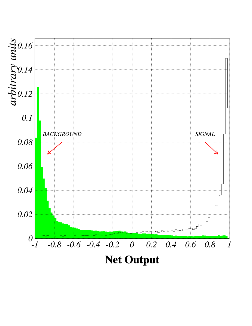
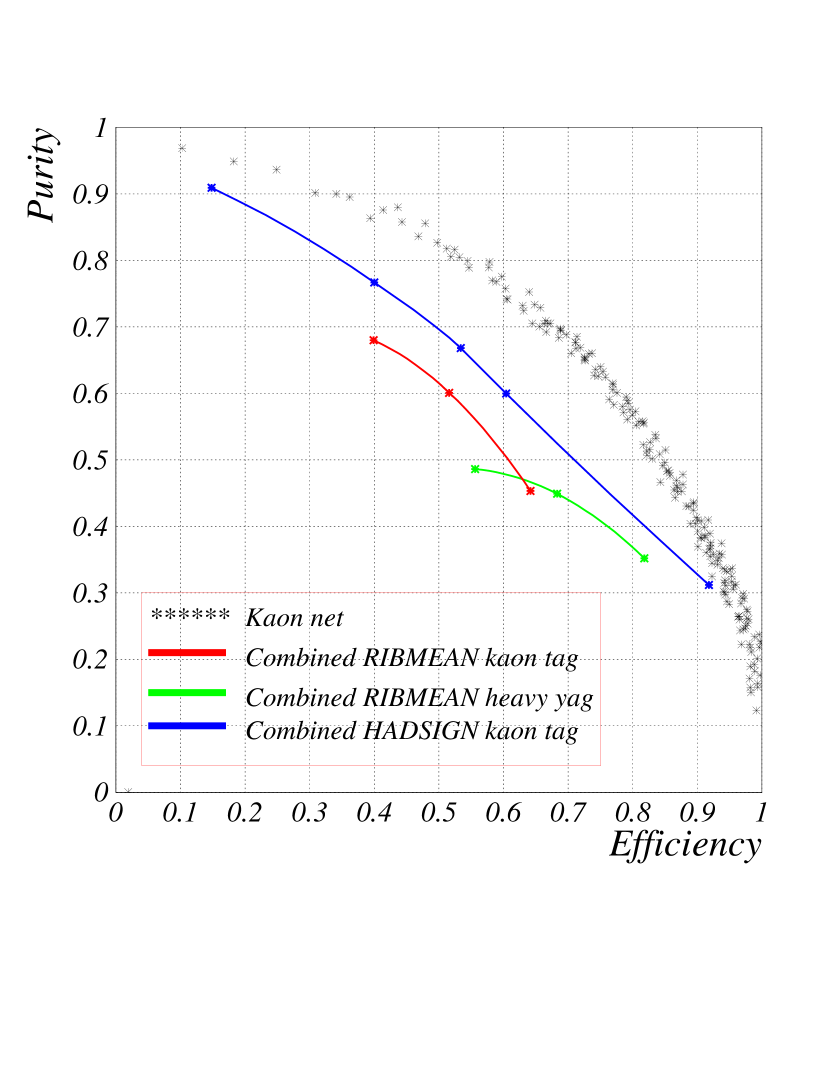
Figure 7: Left: Signal-Background separation of MACRIB for kaons with full RICH information. Signal is accumulated at +1 and background at -1. The separation of the two classes is well done. This allows an efficient separation of kaons from the background, mainly pions. Right: The momentum averaged efficiency purity plot of MACRIB for kaons compared to the combined (RICH gas and liquid + dE/dx) information from HADSIGN and RIBMEAN.

For the separation of background and signal the target of the net outputs were set to -1 and 1 respectively. The output of the net with full RICH information can be seen on the left side of figure 7. A clear separation between kaons and background can be observed. Compared with the combined HADSIGN kaon tag, the combined RIBMEAN kaon tag and RIBMEAN heavy tag one can see that the kaon net of MACRIB has a far better efficiency at the same purity (right side of fig. 7).

As one would expect, the performance of the network without liquid RICH information can not be as good as with the working liquid radiator. The missing information results in a class of particles that lie in the momentum range that is not covered by any detector. These get a net output that lies somewhere between -1 and 1. The bump in the middle of the plot at the left side of figure 8 comes from this class. The comparison with the HADSIGN and RIBMEAN tags shows again a significant improvement. The fact that one can cut on a continuous variable instead of taking discrete tags makes it in addition a more flexible tool.

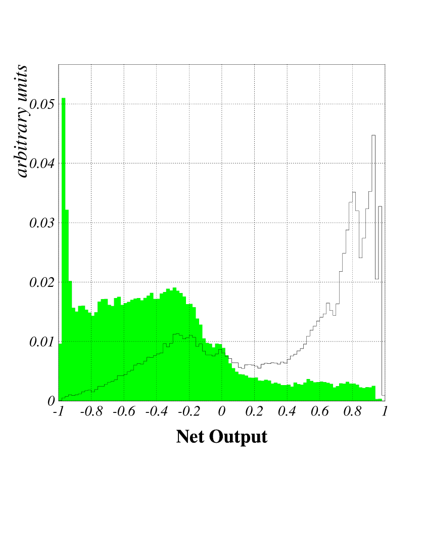
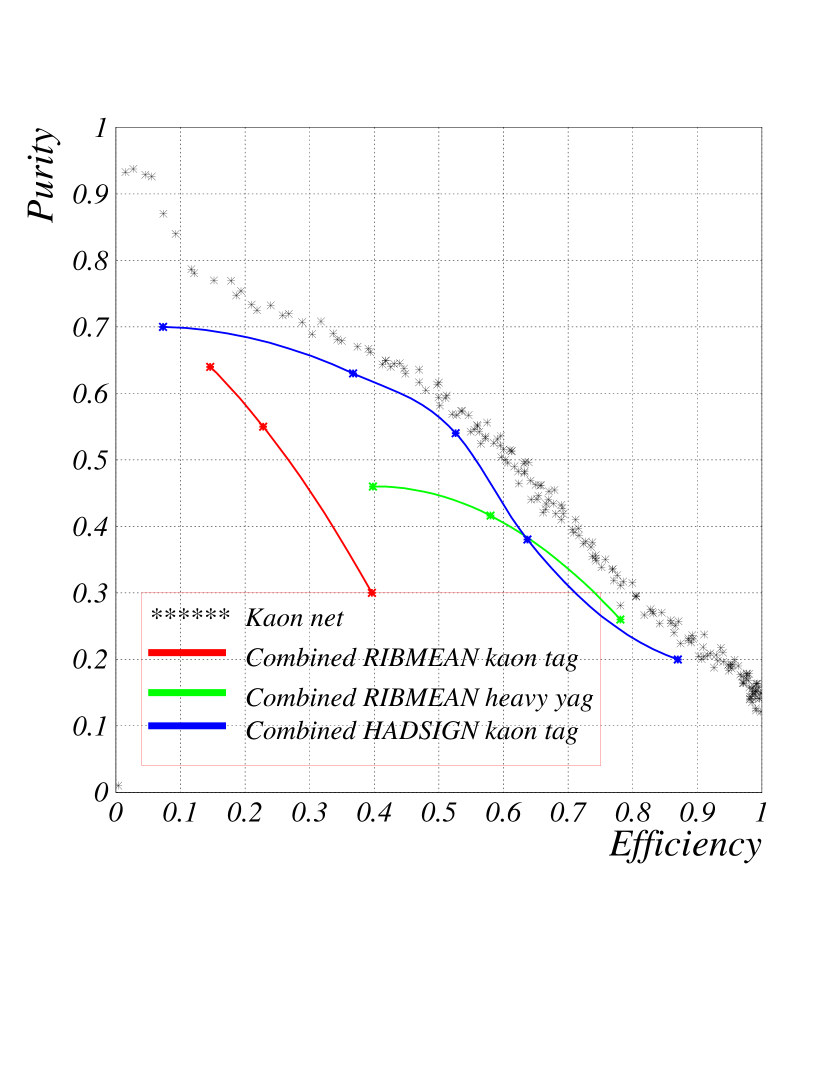
Figure 8: Left: Signal-Background separation of MACRIB for kaons without liquid RICH information. The separation of the two classes can not be done as efficiently as with full RICH information but there is still an improvement compared to the combined RIBMEAN and HADSIGN tags.

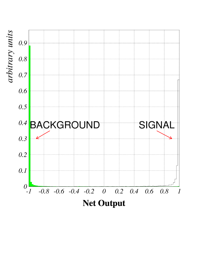
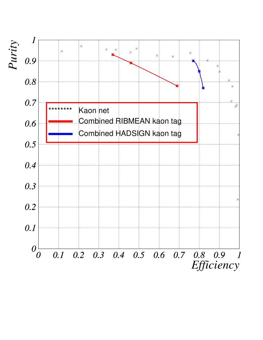
Figure 9: Left: The output of the MACRIB kaon net for low momentum kaons. Both TPC and VD informations have been used as input for the net. Right: The large gain in efficiency compared to RIBMEAN and HADSIGN comes largely from the independent dE/dx information of the vertex detector.

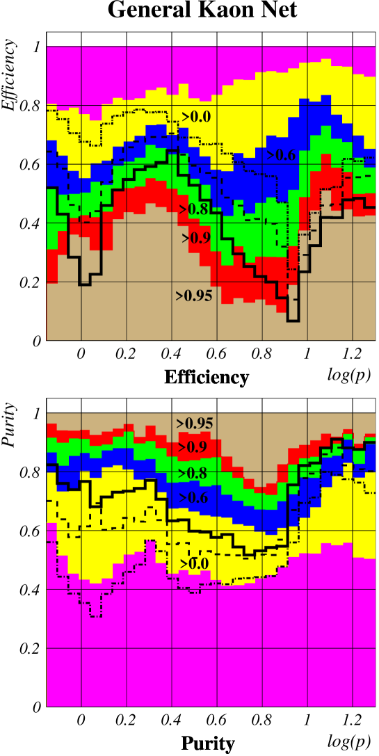
Figure 10: Efficiency and purity of MACRIB vs. momentum for kaons compared to the RIBMEAN performance. The solid line corresponds to the tight kaon tag, the dashed line to the standard kaon tag and the dash-dotted line to the loose tag.

The output of the kaon net below 0.7 GeV is displayed at the left side of figure 9. Since in the TPC the kaon band is well separated from the pion band (see figure 1) a very pure signal to background ratio can be achieved by only considering TPC variables. However, for cases where no TPC measurement is available, HADSIGN and RIBMEAN can provide no tag. This happens, when less then 30 wires are hit or if the kaon pull is larger then two sigmas. By combining the TPC measurement with the information coming from the vertex detector, a very good kaon identification can be achieved even for these particles. This further information is one of the reasons for the large gain in efficiency at same purity compared to the HADSIGN and RIBMEAN tags shown at the right side of figure 9.

Since purity and efficiency depend on momentum the efficiency purity plots in the figures 7,8 and 9 only show the averaged purity and the averaged efficiency in hadronic Z decays. Figure 10 shows the performance of MACRIB over the whole momentum spectrum. The three levels of the combined RIBMEAN kaon tag are compared to different cuts on the kaon net output represented by different colours. The colour codes are the same in both plots for the efficiency and purity. Note that especially the efficiency hole of the RIBMEAN tags below 8 GeV is filled up by MACRIB.

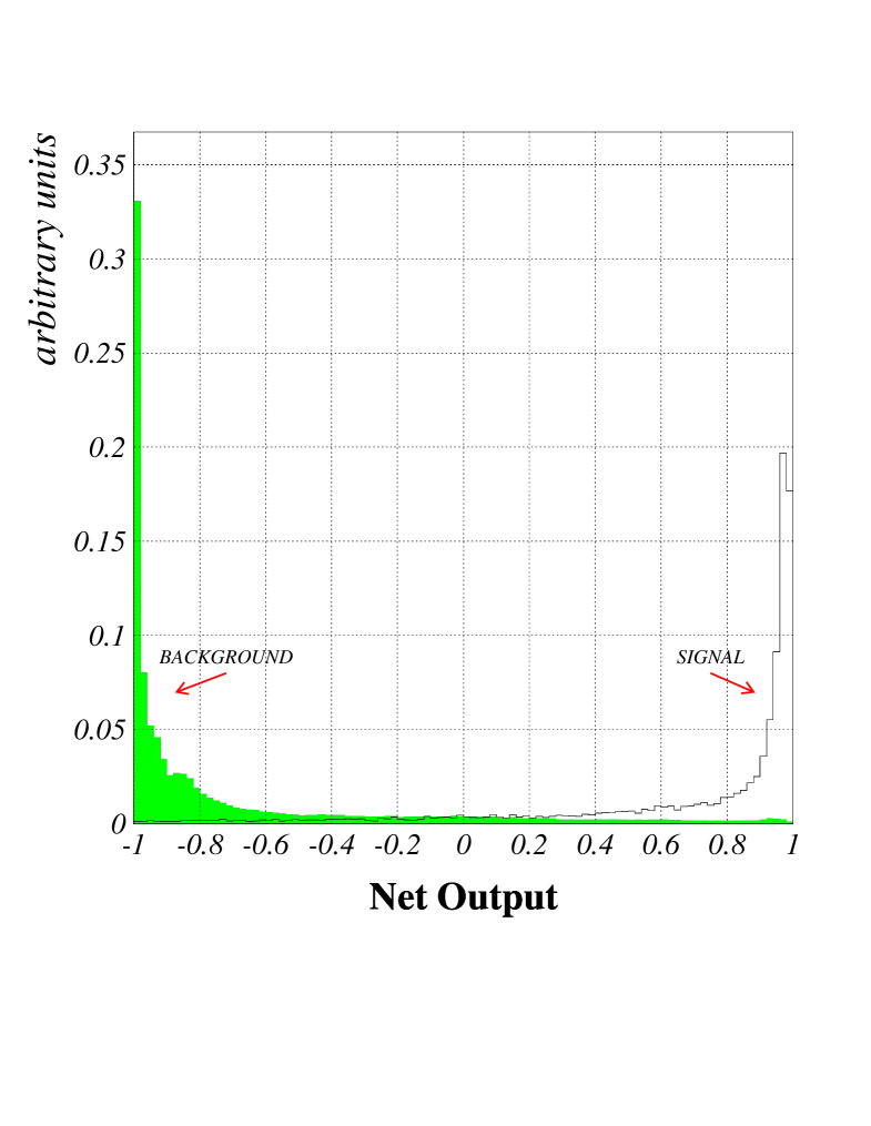
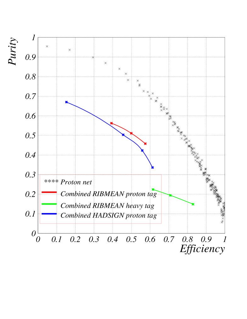
Figure 11: Left: The separation of background and signal of MACRIB for protons. Like for kaons, both classes are well pulled to a peak at -1. and +1. respectively. Right: The purity vs. efficiency of the MACRIB package for protons compared to the performance of the RIBMEAN and HADSIGN tags.

4.2 Proton net

The output of the net with liquid RICH information for protons and background can be seen in 11 together with the comparison of the purity over efficiency plot of the MACRIB routine with that of the combined tags of RIBMEAN and HADSIGN. At high purity a large gain in efficiency is achieved.

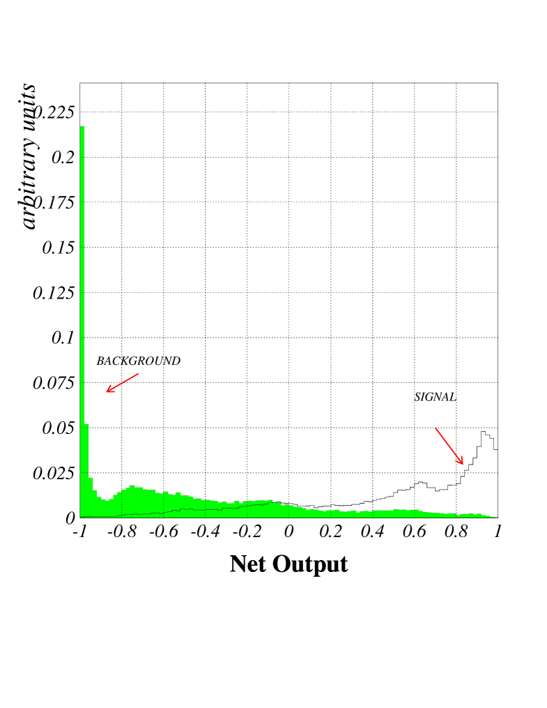
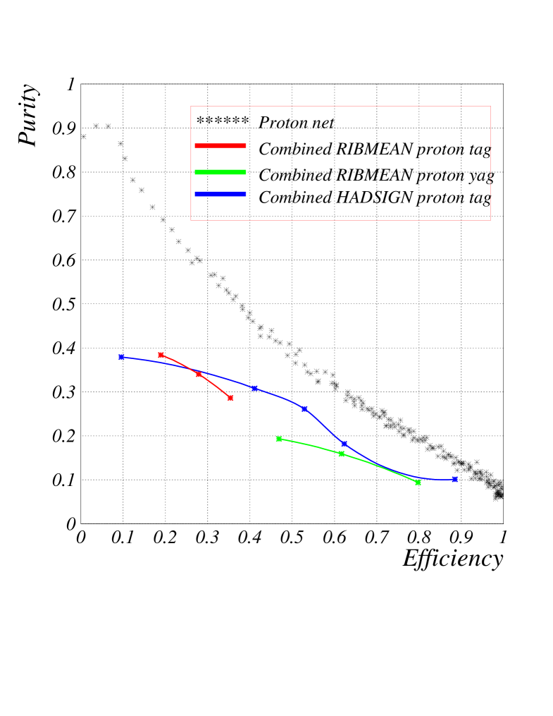
Figure 12: Left: The separation of background and signal of MACRIB for protons. Like for kaons, both classes are well pulled to a peak at -1. and +1. respectively. Right: The purity vs. efficiency of the MACRIB package for protons compared to the performance of the RIBMEAN and HADSIGN tags.

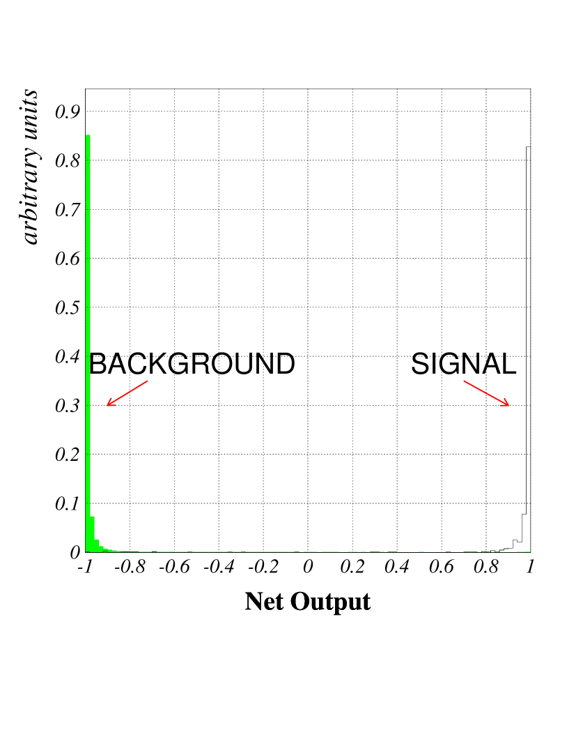
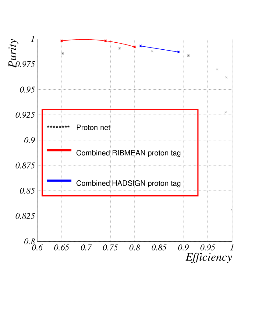
Figure 13: Left: Signal and background are accumulated at the extreme ends of the net output plot. Right: Due to the very good separability of protons from background a very high level of purity and efficiency can be achieved. Note that only a small window of the efficiency purity plot is shown. MACRIB has a better efficiency than the RIBMEAN and HADSIGN tags, due to the additional VD information.

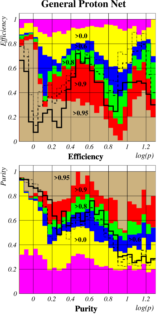
Figure 14: Efficiency and purity of MACRIB vs. momentum for protons compared to the RIBMEAN performance. The solid line corresponds to the tight proton tag, the dashed line to the standard proton tag and the dash-dotted line to the loose tag.

As for the kaons, the performance of the net goes down if no liquid RICH information is available. Though, the proton net deals better with the loss of this information than the kaon net. This lies in the fact that the VD dE/dx bands of protons and pions are still separated in the momentum region usually covered by the liquid radiator. The bump, representing the class of particles with no detector information or with ambiguous information, in the middle of the performance plot at the left side of figure 12 can be found here too, but at a lower level than for the kaon net. The efficiency purity plot shows the possibility of going to very pure proton samples. This option was not available with the RIBMEAN and HADSIGN tags, as can be seen at the right side of figure 12.

For particles with momenta below 0.7 GeV the net output is shown in figure 13 (left). The proton and pion bands are separated by many sigmas in both the TPC and vertex detectors. This makes a very pure and efficient identification possible. The comparison between MACRIB, RIBMEAN and HADSIGN can be seen at the right side of the same figure. The particles having no RIBMEAN or HADSIGN tags contribute to the efficiency gain in MACRIB, by utilising the independent dE/dx measurement provided by the VD.

The momentum dependence of the efficiency and purity can be seen in figure 14 together with the loose, standard and tight tags of the RIBMEAN routine.

4.3 Simulation-Data Agreement

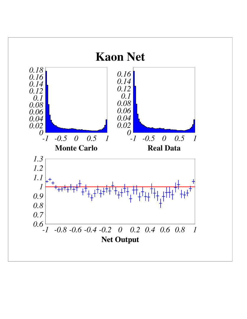
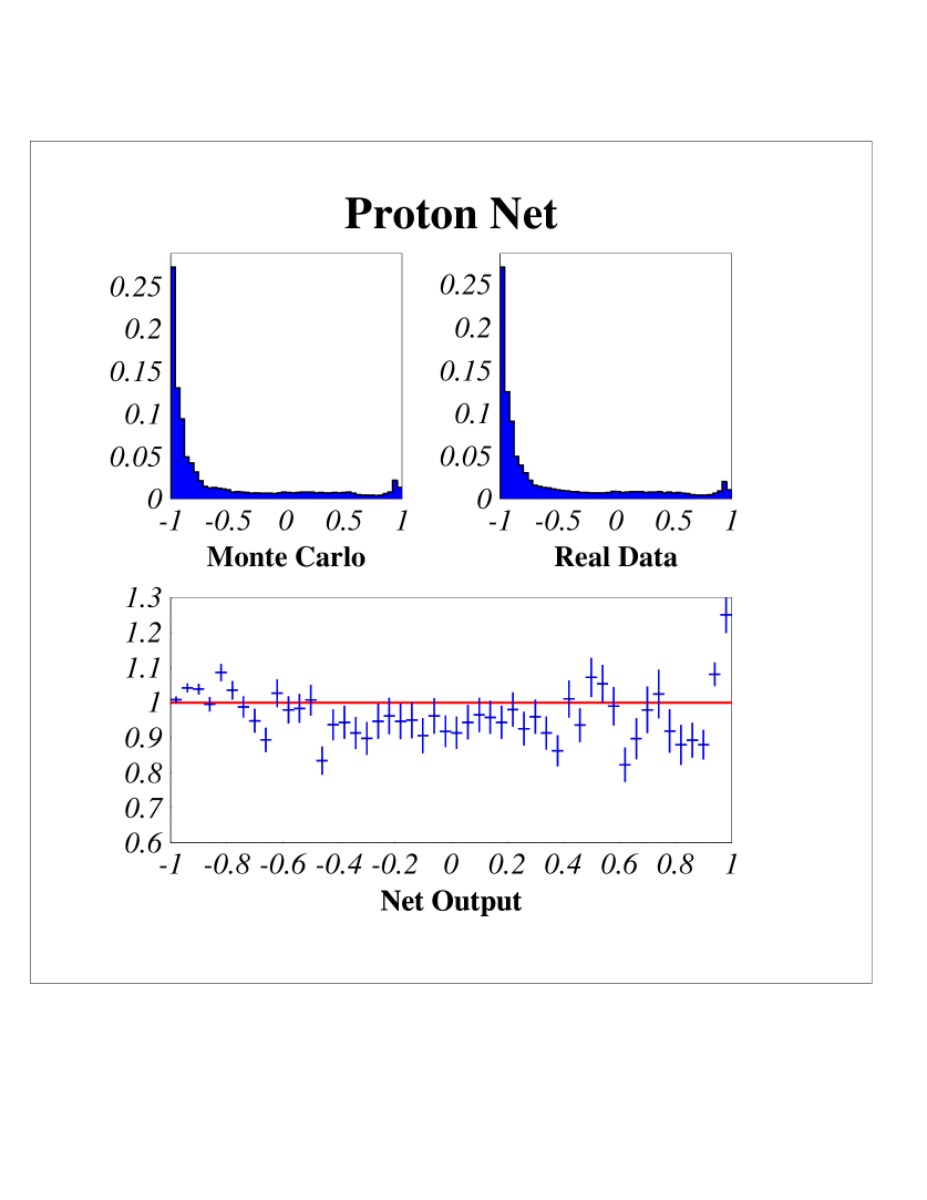
Figure 15: Left: The output of MACRIB for kaons for an independent MC sample and real data. Below the ratio of the normalised distributions can be seen (MC divided by the real data). Right: The output of MACRIB for protons, with the ratio of the normalised distributions.

For the test of the Simulation-Data agreement of the network output we used an independent Monte Carlo sample, which has not been used in the training of the nets. For the case of fully working RICH detectors the comparison between real data and Monte Carlo is shown in figures 15. The distributions have been normalised and the simulated sample divided by the real data. The agreement is reasonable over most of the network output range. At the far ends of the plot a surplus of the MC can be observed. This is due to the more ideal conditions of the simulation, so that the net can assign an output value closer to the edges.

5 MACRIB - How to get the net output

We have written a simple stand-alone-routine MACRIB returning the kaon- and the proton-net outputs for a given track with the PA-pointer LPA. This routine is included in the BSAURUS package, since it uses the network routines of BSAURUS. The user has to include the BSAURUS library by including BSAURUS into the argument list of dellib in the link step of the job in order to have access to the routine.
Before calling MACRIB for a track one first has to call once per event[3]:

• CALL RICHID

• CALL RIDECR

• CALL GETMINE(MYTYPE)
  where MYTYPE=1 means LPA/tanagra, MYTYPE=2 means VECSUB

After that MACRIB can be called with the input argument LPA:

CALL MACRIB(LPA,XKAONNET,XPROTONNET)

BSAURUS users can access the net outputs via the BSAURUS commons

BSPAR(IBP_MACK,IPART) BSPAR(IBP_MACP,IPART)

on the track basis. The output variables are the kaon net output XKAONNET and the proton net output XPROTONNET. They are real variables with values between -1. and 1. XKAONNET/XPROTONNET $\to$ -1. means identification as not a kaon/proton whereas XKAONNET/XPROTONNET $\to$ 1. means identified as kaon/proton. Tracks that fail to pass the cuts in MACRIB get the value -2.

6 Sample plots

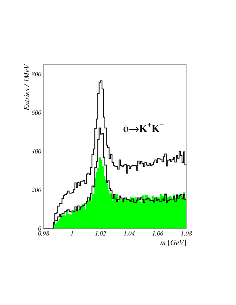
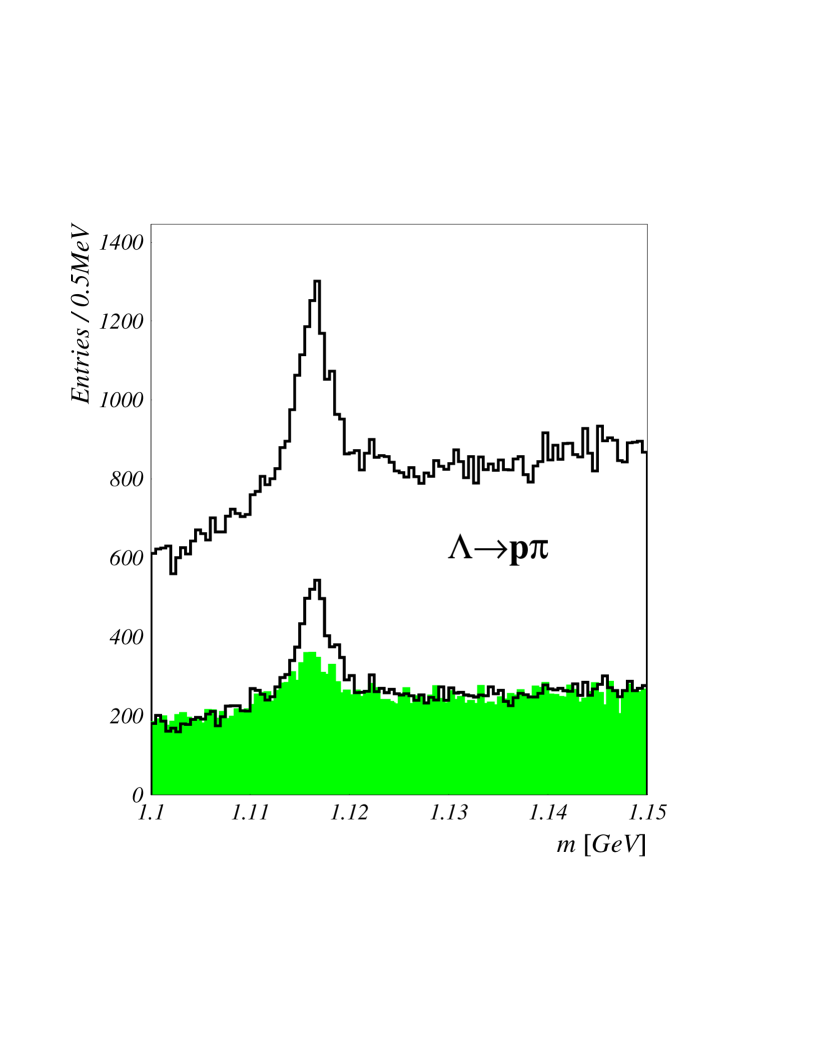
Figure 16: Left: Comparison of reconstructed $\Phi$ mesons obtained by MACRIB (solid line) and the RIBMEAN routine (shaded area). The RIBMEAN result is compared to the signal given by MACRIB at the same background level (lower solid line) and at the same purity. At the same background level about 56% more $\phi$ events are selected corresponding to a purity increase of 16%. At the same purity the tagging efficiency is doubled.
Right: The comparison between MACRIB and HADSIGN in the $\Lambda\to p\pi$ decay. The solid line represents again the distribution by MACRIB and the shaded area comes from HADSIGN. For the distribution no cuts at all have been applied, in particular no decay length cut. At the same background level the efficiency to tag a $\Lambda$ is more than doubled. At the same purity the ratio is about 4.

The kaon network was tested on real data to observe the gain in efficiency in physically relevant decays. The gain in efficiency is always dependent on the momentum region of the decay products, as the networks are momentum dependent too, in their performance.

$\Phi$ mesons were reconstructed by identifying both kaons in the decay $\Phi\to K^{+}K^{-}$. Using a cut of 0.8 in MACRIB’s kaon network output for both tracks, about 56 % more $\Phi$’s are selected than with the combined RIBMEAN tight heavy tag at the same background level. The purity at this cut is about 60% for the signal obtained by the RIBMEAN tagging routine and approximately 70% in the distribution achieved by MACRIB (figure 16 Left). The efficiency gain at the same purity is thus much higher ($\approx 2$).

In the decay $\Lambda\to p\pi$ the output of HADSIGN has been compared to that of MACRIB. At the same background level a large gain can be observed, in this case too (figure 16 Right). For the distribution no cuts were applied at all, beside the proton tagging. This explains the relatively large background level. At the same purity the tagging efficiency of MACRIB is four times as large as that of HADSIGN.

In the decay $D_{s}\to\phi\pi$ (figure 17) RIBMEAN provides a comparable output to that of MACRIB, since a very pure $\phi$ enrichment is possible without any kaon tagging. The decay of the $D_{s}$ meson into $K^{*}K$ is shown in figure 18. It compares the output of MACRIB and RIBMEAN at same purities for data taken in the years 1994-1995 and 1992-1993. The efficiency gain is about 30% and 100% respectively.

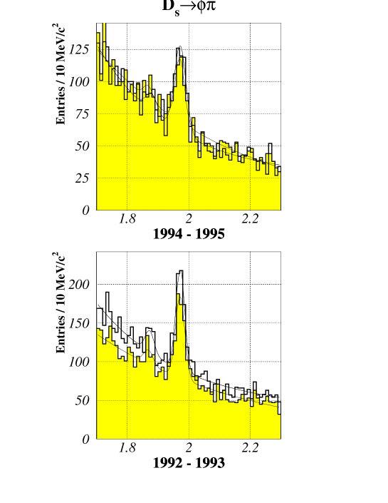
Figure 17: Comparison of reconstructed $D_{s}$ mesons decaying into $\phi\pi$ obtained by MACRIB (solid line) and the RIBMEAN routine (shaded area). The efficiency of tagging is in the case of MACRIB slightly better than in the case of RIBMEAN.

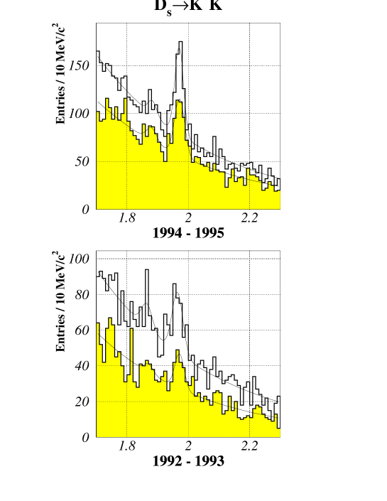
Figure 18: Comparison of reconstructed $D_{s}$ mesons decaying into $K^{*}K$ obtained by MACRIB (solid line) and the RIBMEAN routine (shaded area). The plots show distributions at same purities. The efficiency gain for the data taken in the years 94-95 is about 33% (above) and for the data taken in the years 92-93 about 100% (below).

7 Acknowledgements

Compared to the first version presented in the October 1998 DELPHI analysis week, the net was still much improved, also due to implementation of feedback obtained from RICH experts, especially Claire Bourdarios and Emile Schyns, during that week. Many thanks to them.

We want to thank Jong Yi for providing the $\Phi$ and $D^{*}$ plots and Oleg Kuznets for providing the $D_{s}$ plots.

References

- [1] P. M. Kluit. Particle identification combining the RICHes and the TPC.
- [2] M. Battaglia, P. M. Kluit. Particle identification using the RICH detectors based on the RIBMEAN package. DELPHI 96-133 RICH 90, 16 Sep 96 and 21 March 97.
- [3] The RICH group and hadident task. User guide of the HADIDENT/RICH software.
-
[4]
W. Adam et al.
Analysis techniques for the DELPHI ring imaging Cherenkov detector. and the
references there
DELPHI 94-112 PHYS 429, 1st June 1994. -
[5]
P. Abreu et al.
Charged kaon production in tau decays at LEP
Phys. Lett B 334 (1994) 435.