New empirical fits to the proton electromagnetic form factors

Abstract

Recent measurements of the ratio of the elastic electromagnetic form factors of the proton, G_Ep/G_Mp, using the polarization transfer technique at Jefferson Lab show that this ratio decreases dramatically with increasing Q², in contradiction to previous measurements using the Rosenbluth separation technique. Using this new high quality data as a constraint, we have reanalyzed most of the world $ep$ elastic cross section data. In this paper, we present a new empirical fit to the reanalyzed data for the proton elastic magnetic form factor in the region 0 $<$ $Q^{2}$ $<$ 30 GeV². As well, we present an empirical fit to the proton electromagnetic form factor ratio, G_Ep/G_Mp, which is valid in the region 0.1 $<$ $Q^{2}$ $<$ 6 GeV².

The elastic electromagnetic form factors are crucial to our understanding of the proton’s internal structure. Indeed, the differential cross section for elastic $ep\rightarrow ep$ scattering is described completely in terms of the Dirac and Pauli form factors, $F_{1}$ and $F_{2}$, respectively, based solely on fundamental symmetry arguments. Further, the Sachs form factors, $G_{Ep}$ and $G_{Mp}$, which are simply derived from $F_{1}$ and $F_{2}$, reflect the distributions of charge and magnetization current within the proton.

Until recently, the form factors of the proton have been determined experimentally using the Rosenbluth separation method [4], in which one measures elastic $ep$ cross sections at constant $Q^{2}$, and varies both the beam energy and scattering angle to separate the electric and magnetic contributions. In terms of the Sachs form factors, the differential cross section for elastic $ep$ scattering has traditionally been written as

$$\frac{d\sigma}{d\Omega}=\sigma_{ns}\left(\frac{G_{Ep}^{2}+\tau G_{Mp}^{2}}{1+\tau}+2\tau G_{Mp}^{2}\tan^{2}(\theta_{e}/2)\right),$$ (1)

where $\tau=Q^{2}/4M_{p}^{2}$, $\theta_{e}$ is the in-plane electron scattering angle. For elastic $ep$ scattering, the so-called nonstructure cross section, $\sigma_{ns}$ is given by

$$\sigma_{ns}=\frac{\alpha_{em}^{2}\cos^{2}(\theta_{e}/2)}{4E^{2}\sin^{4}(\theta_{e}/2)}\frac{E^{\prime}}{E}$$ (2)

where $\alpha_{em}$ is the electromagnetic coupling constant, and $E^{\prime}$($E$) is the energy of the scattered (incident) electron.

From the measured differential cross section, one typically derives a “reduced cross section”, defined according to

$$\sigma_{R}=\frac{d\sigma}{d\Omega}\frac{(1+\tau)\epsilon}{\sigma_{ns}\tau}=\frac{\epsilon}{\tau}G_{Ep}^{2}(Q^{2})+G_{Mp}^{2}(Q^{2}),$$ (3)

where $\epsilon=\{1+2(1+\tau)\tan^{2}(\theta_{e}/2)\}^{-1}$ is a measure of the virtual photon polarization. Equation 3 is known as the Rosenbluth formula, and shows that fits to reduced cross section measurements made at constant $Q^{2}$ but varying $\epsilon$ values may be used to extract both form factors independently.

With increasing $Q^{2}$, the reduced cross sections are increasingly dominated by the magnetic term $G_{Mp}$; at $Q^{2}$ $\approx$ 3 GeV², the electric term contributes only a few percent of the cross section. Furthermore, referring to the open data points in the left panel of Fig. 1, one can see that the various Rosenbluth separation data sets [5, 6, 7, 8, 9, 10] for the ratio $\mu_{p}G_{Ep}/G_{Mp}$, where $\mu_{p}=2.79$ is the magnetic moment of the proton, are not consistent with one another for $Q^{2}$ $>$ 1 GeV². It is clear that a tremendous effort has gone into the analysis of these difficult experiments, however, one is forced to speculate that some of the experiments have underestimated the systematic errors. For example, the Rosenbluth experiments apply radiative corrections to their data at leading order, i.e. one hard photon emitted, which can vary significantly with $\epsilon$ depending on the specific experiment. However, higher order radiative corrections, i.e. involving more than one photon, could in fact change the slope of the reduced cross section versus $\epsilon$ plot, and thus have an impact on the extracted form factor ratio.

Due to the fundamental nature of the quantities at hand, a more robust method for measuring the proton electromagnetic form factors is certainly desirable. Over the last few years, focal plane polarimeters have been installed in hadron spectrometers in experimental facilities at Bates, Mainz, and Jefferson Lab. Specifically, one makes use of the polarization transfer method [12, 13], in which one measures, using a focal plane polarimeter, the transverse ($P_{t}$) and longitudinal ($P_{\ell}$) components of the recoil proton polarization in ${}^{1}H(\vec{e},e^{\prime}\vec{p})$ scattering, using a longitudinally polarized electron beam.

The proton form factor ratio is given simply by

$$r=\mu_{p}{G_{Ep}\over G_{Mp}}=-{P_{t}\over P_{\ell}}{\mu_{p}\left(E_{e}+E_{e^{\prime}}\right)\over 2M_{p}}\tan\left(\theta_{e}/2\right).$$ (4)

Here, $E_{e}$ ($E_{e^{\prime}}$) is the incident (scattered) electron energy. The polarization transfer method offers a number of advantages over the traditional Rosenbluth separation technique. Using the ratio of the two simultaneously measured polarization components greatly reduces systematic uncertainties. For example, a detailed knowledge of the spectrometer acceptances, something which plagues the cross section measurements, is in general not needed. Moreover, it is not necessary to know either the beam polarization or the polarimeter analyzing power, since both of these quantities cancel in measuring the ratio of the form factors. The dominant systematic uncertainty is the knowledge of spin transport, although in comparison to the size of the systematic uncertainties in cross section measurements, this too is small. Finally, the most recent theoretical calculations [20] of the effects of radiative processes verify the assertion that the form factor ratio is unaffected at the momentum transfers involved here.

FIG. 1.: (a) Published world data for $r=\mu_{p}G_{Ep}/G_{Mp}$; open symbols indicate Rosenbluth separations [5, 6, 7, 8, 9, 10] while filled symbols indicate polarization transfer measurements [2, 3, 14, 15, 16]. In the case of the Rosenbluth data, the error bars shown are the result of combining systematic and statistical errors in quadrature. For the polarization transfer measurements, the error bars shown are statistical only; the systematic uncertainties are in general a small fraction of the statistical error in these experiments. The dot dash line is the parameterization from ref. [17] to the cross section data, which indicates $r$ $\approx$ $1$. (b) Fit to polarization transfer measurements from Jefferson Lab. Included are the most recent data at large $Q^{2}$ from E99007 [3]. Also shown are calculated ratios from recent fits to the electromagnetic form factors by Lomon [18] within the Gari-Krümpelmann framework.

As mentioned above, the proton form factor ratio has been measured at several facilities using the polarization transfer technique. It was first used by Milbrath et al. [14], who determined $r$ at $Q^{2}$ = 0.38 and 0.50 GeV², and the result was in good agreement with both the Rosenbluth separation results and a subsequent polarization measurement at $Q^{2}$ = 0.4 by Dieterich et al. [15] at Mainz. However, polarization transfer measurements up to $Q^{2}$=3.5 GeV² in Hall A at Jefferson Lab [2, 16] have revealed the somewhat surprising result shown in Fig. 1, that the form factor ratio decreases with increasing $Q^{2}$. Most recently, this trend has been confirmed in Jefferson Lab Experiment E99007 [3], which extends the form factor ratio measurement to $Q^{2}$=5.6 GeV²; these new data are also shown in Fig. 1. We have fit the Jefferson Lab data using a simple linear parameterization, i.e.,

$$r=1.0-(0.130\pm 0.005)\left[Q^{2}-(0.04\pm 0.09)\right],$$ (5)

for 0.04 $<$ $Q^{2}$ $<$ 5.6 GeV². This empirical description, which gives an acceptable fit to the Jefferson Lab data with the smallest number of free parameters, is shown in the right panel of Fig. 1 using two dashed curves to represent the range of uncertainty in the fit parameters. Note that this description of the ratio is singularly inconsistent with the global fit from Ref. [17] shown in the left panel of Fig. 1. However, a similar decreasing ratio has been reported in a number of recent theoretical models. In addition, we also show in the right panel of Fig. 1 ratios calculated from recent fits to the electromagnetic form factors by Lomon [18] within the framework of the Gari-Krümpelmann model. The two curves shown differ somewhat from one another in their specific choice of the form of the hadronic form factors as well as in the parametrization of the behaviour at large $Q^{2}$, and as such represent upper and lower bounds on the extracted form factor ratio. However, these curves both lie significantly above the new data.

In the remainder of this paper, for the purposes of reanalyzing the cross section data, we have used an empirical prescription for the form factor ratio. For $Q^{2}$ $<$ 0.04 GeV², we have used $r=1$; for 0.04 $<$ $Q^{2}$ $<$ 7.7 GeV², we have employed Eq. 5; for $Q^{2}$ $>$ 7.7 GeV², we have used $r=0$. The boundary of 0.04 GeV² (7.7 GeV²) corresponds to the value of $Q^{2}$ where Eq. 5 predicts a ratio of 1 (0). The choice of setting $r=0$ for the largest $Q^{2}$ region is somewhat arbitrary, since no experimental data exists in this kinematic regime. However, since the electric contribution to the total cross section is minimal in this $Q^{2}$ region, our choice has in fact little impact on the extracted value of the magnetic form factor. In addition, our linear fit almost certainly has the wrong asymptotic behavior at very large $Q^{2}$, based on theoretical expectations, and therefore we have extended the empirical fit only to $Q^{2}$=7.7 GeV² to match the higher $Q^{2}$ assumption of $r=0$.

As stated above, the new Jefferson Lab data for the form factor ratio is in general disagreement with the higher $Q^{2}$ Rosenbluth separation measurements. Since the Rosenbluth separation measurements systematically attribute more strength in the cross section to the electric part (larger ratio, $r$), this means that their extracted values for the magnetic form factor, $G_{Mp}$, are potentially systematically too small.

We have reanalyzed the available cross section data using the following procedure:

• In the cases where experiments have extracted reduced cross section data at multiple $\epsilon$ values at each $Q^{2}$ (Refs. [5, 6, 7, 8, 10, 11]), we have reanalyzed these data using the aforementioned form factor ratio prescription. The net effect of this procedure is that the form factor ratio constraint fixes the ratio of the slope to the intercept of the graph of reduced cross section vs. $\epsilon$. Therefore, in practice, one extracts only a single parameter from the new fit to the data.

• For the data of Sill et al. [19], which presents reduced cross section data at a single $\epsilon$ value for each $Q^{2}$, we extract $G_{Mp}$ using the above form factor ratio prescription directly. The authors had assumed, quite reasonably at the time, $r=1$ in their extraction of $G_{Mp}$.

• It is important to recognize that Eqs. 1 and 2 describe the elementary single photon exchange electron scattering cross section, i.e., the Born cross section. However, other processes, such as vacuum polarization and radiative effects, contribute to the total cross section that one measures in an experiment. The technique that has been used to date is to correct the measured $ep$ cross section to account for the contribution from these extra processes, which are fully calculable within the framework of quantum electrodynamics, and thus extract the Born cross section [21]. This being stated, the calculation of the vacuum polarization processes has varied between the different experiments. Specifically, only the most recent analyses [5, 10, 19] have included the $\mu^{+}\mu^{-}$ and $q\bar{q}$ vacuum polarization contributions. These processes were not accounted for in the original work of Mo and Tsai [21]. As a result, in our reanalysis of the cross section data we have included, using the same formalism as presented in [10], a correction to the extracted Born cross sections in the older experiments [6, 7, 8, 11]. The size of this correction is almost negligible for $Q^{2}$ $<$ 0.3 GeV², but increases to about 1.3% at Q²=4 GeV², which is the largest momentum transfer probed in the earlier measurments. We also point out that in the hadronic and particle physics communities, the vacuum polarization processes are often modelled in terms of a strengthening of the electromagnetic coupling, or alternatively in terms of a “screening” of the bare electron charge at low $Q^{2}$.

As an example of the effect of form factor ratio constraint, in Fig. 2, we show reduced cross section data which has been recalculated using the original data from Andivahis et al. for the four lowest $Q^{2}$ values of 1.75, 2.50, 3.25, and 4.00 GeV². In each case, the dashed line is the best fit line using the direct Rosenbluth method. The solid line is the best fit using our form factor ratio constraint. The error bars shown are statistical and point-to-point systematic errors, as reported in Ref. [5], added in quadrature. The open and closed symbols in the figure are from two different spectrometers, known as the “1.6 GeV” and “8 GeV” spectrometers, respectively. In Ref. [5], the authors report that the data from these two spectrometers were cross-normalized at the two lowest $Q^{2}$ points, which resulted in a renormalization factor of $0.956$ being applied to the 1.6 GeV spectrometer data. In this paper, the authors also report an overall normalization uncertainty of $\delta_{norm}=1.77\%$. We have not included the renormalization uncertainty in each data point, but it has been included in the final uncertainty in the intercept of each graph, as

$$(\delta b_{final})^{2}=(\delta b_{raw})^{2}+(b_{raw}\cdot\delta_{norm})^{2},$$ (6)

where $b_{raw}$ is the intercept of the straight-line fit to the data.

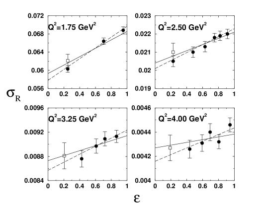
FIG. 2.: The reduced cross section data of Andivahis et al. for the four lowest $Q^{2}$ values of 1.75, 2.50, 3.25, and 4.00 GeV². The open and closed symbols in the figure are from two different spectrometers. The solid (dashed) line represents the fit using the form factor ratio constraint (direct extraction method). The details of the fitting procedure, as well as the calculation of uncertainties and normalization factors, are discussed in text.

We note that our new fits would correspond to increasing the normalization factor of the 1.6 GeV spectrometer, or alternatively introducing a momentum dependence to the 1.6 GeV spectrometer acceptance. In an attempt to address this issue, we have used instead a renormalization factor of $0.980$ for the 1.6 GeV data, which represents an upper limit derived from the original normalization factor and uncertainty from Ref. [5].

In addition, in the final extraction of $G_{Mp}$ using the form factor ratio constraint, we have incorporated (in quadrature) the uncertainty in the form factor ratio itself, as expressed in Eq. 5. The results of the two extraction methods, including the final uncertainties, are summarized in Table I.

TABLE I.: Compilation of all $\frac{G_{M_{p}}}{\mu_{p}G_{D}}$ extraction results. The details of the procedure for determing uncertainties and renormalization factors are discussed in the text.

$Q^{2}\atop(\rm{GeV}^{2})$	Direct Extraction	New Extraction	$Q^{2}\atop(\rm{GeV}^{2})$	Direct Extraction	New Extraction
	Andivahis et al.[5]			Berger et al.[7]
1.750	1.053 $\pm$ 0.013	1.067 $\pm$ 0.010	0.389	0.985 $\pm$ 0.027	0.986 $\pm$ 0.021
2.500	1.058 $\pm$ 0.012	1.066 $\pm$ 0.010	0.584	0.985 $\pm$ 0.021	1.002 $\pm$ 0.021
3.250	1.053 $\pm$ 0.015	1.063 $\pm$ 0.010	0.779	1.005 $\pm$ 0.024	1.015 $\pm$ 0.021
4.000	1.040 $\pm$ 0.015	1.053 $\pm$ 0.010	0.973	1.005 $\pm$ 0.026	1.035 $\pm$ 0.022
5.000	1.028 $\pm$ 0.015	1.035 $\pm$ 0.010	1.168	1.024 $\pm$ 0.031	1.051 $\pm$ 0.023
6.000	1.002 $\pm$ 0.019	1.012 $\pm$ 0.011	1.363	1.038 $\pm$ 0.030	1.044 $\pm$ 0.023
7.000	0.973 $\pm$ 0.022	1.002 $\pm$ 0.013	1.558	1.032 $\pm$ 0.034	1.062 $\pm$ 0.024
	Bartel et al.[6]		1.752	1.064 $\pm$ 0.042	1.066 $\pm$ 0.025
0.670	0.964 $\pm$ 0.027	1.006 $\pm$ 0.014		Janssens et al.[11]
1.000	1.014 $\pm$ 0.028	1.056 $\pm$ 0.015	0.156	0.926 $\pm$ 0.027	0.979 $\pm$ 0.013
1.169	1.017 $\pm$ 0.024	1.052 $\pm$ 0.014	0.179	0.960 $\pm$ 0.016	0.968 $\pm$ 0.009
1.500	1.031 $\pm$ 0.030	1.065 $\pm$ 0.015	0.195	1.001 $\pm$ 0.026	0.998 $\pm$ 0.013
1.750	1.052 $\pm$ 0.023	1.052 $\pm$ 0.015	0.234	0.937 $\pm$ 0.025	0.985 $\pm$ 0.011
3.000	1.052 $\pm$ 0.023	1.052 $\pm$ 0.014	0.273	0.940 $\pm$ 0.017	0.961 $\pm$ 0.009
	Litt et al.[8]		0.292	0.934 $\pm$ 0.020	0.965 $\pm$ 0.009
1.500	0.972 $\pm$ 0.114	1.071 $\pm$ 0.022	0.312	0.966 $\pm$ 0.016	0.965 $\pm$ 0.009
2.000	0.979 $\pm$ 0.074	1.070 $\pm$ 0.022	0.350	0.973 $\pm$ 0.025	0.973 $\pm$ 0.012
2.500	1.011 $\pm$ 0.034	1.064 $\pm$ 0.022	0.389	0.958 $\pm$ 0.014	0.983 $\pm$ 0.008
3.750	0.971 $\pm$ 0.041	1.072 $\pm$ 0.022	0.428	0.969 $\pm$ 0.024	0.998 $\pm$ 0.012
	Sill et al.[19]		0.467	0.976 $\pm$ 0.016	0.994 $\pm$ 0.009
2.862	1.023 $\pm$ 0.018	1.063 $\pm$ 0.021	0.506	0.957 $\pm$ 0.024	0.988 $\pm$ 0.012
3.621	1.024 $\pm$ 0.020	1.060 $\pm$ 0.023	0.545	0.986 $\pm$ 0.016	1.001 $\pm$ 0.009
5.027	1.007 $\pm$ 0.018	1.040 $\pm$ 0.019	0.584	0.982 $\pm$ 0.024	1.003 $\pm$ 0.012
4.991	1.011 $\pm$ 0.019	1.042 $\pm$ 0.021	0.623	0.989 $\pm$ 0.016	0.997 $\pm$ 0.008
5.017	1.000 $\pm$ 0.018	1.027 $\pm$ 0.019	0.662	1.028 $\pm$ 0.025	1.017 $\pm$ 0.012
7.300	0.949 $\pm$ 0.019	0.973 $\pm$ 0.020	0.701	0.984 $\pm$ 0.017	1.009 $\pm$ 0.009
9.629	0.891 $\pm$ 0.019	0.907 $\pm$ 0.020	0.740	1.017 $\pm$ 0.025	1.039 $\pm$ 0.012
11.99	0.873 $\pm$ 0.019	0.885 $\pm$ 0.020	0.779	1.037 $\pm$ 0.018	1.023 $\pm$ 0.009
15.72	0.821 $\pm$ 0.026	0.829 $\pm$ 0.025	0.857	1.086 $\pm$ 0.018	1.068 $\pm$ 0.011
19.47	0.732 $\pm$ 0.028	0.738 $\pm$ 0.029		Walker et al.[10]
23.24	0.729 $\pm$ 0.033	0.734 $\pm$ 0.033	1.000	1.002 $\pm$ 0.028	1.045 $\pm$ 0.011
26.99	0.710 $\pm$ 0.041	0.713 $\pm$ 0.042	2.003	1.016 $\pm$ 0.013	1.076 $\pm$ 0.011
31.20	0.721 $\pm$ 0.064	0.723 $\pm$ 0.064	2.497	1.011 $\pm$ 0.013	1.075 $\pm$ 0.011
			3.007	1.003 $\pm$ 0.013	1.072 $\pm$ 0.010

In Fig. 3, we show data for the proton magnetic form factor, expressed as $G_{Mp}/\mu_{p}G_{D}$, where $G_{D}=(1+Q^{2}/0.71)^{-2}$ is the dipole form factor parameterization. In the left panel, we show the magnetic form factor as extracted using direct Rosenbluth separation (or using the assumption of $r=1$ in the case of the data of Sill et al.). In the right panel, we show the newly extracted data using the above constraint on the form factor ratio. In both panels, the dashed curve is the parameterization of Bosted [17], while in the right panel, the solid line is our new empirical fit, and is given by

$$\frac{G_{Mp}}{\mu_{p}}=\frac{1}{1+(0.116\pm 0.040)Q+(2.874\pm 0.098)Q^{2}+(0.241\pm 0.107)Q^{3}+(1.006\pm 0.069)Q^{4}+(0.345\pm 0.017)Q^{5}},$$ (7)

the form of which is consistent with Ref.[17].

FIG. 3.: a) The proton magnetic form factor, expressed as $G_{Mp}/\mu_{p}G_{D}$, as published in the literature. b) The proton magnetic form factor, after reanalysis using the form factor ratio constraint. The solid line is the new empirical fit, as explained in the text, while the dashed line is the parameterization from Ref. [17].

Imposing the form factor ratio constraint has the expected effect that the extracted magnetic form factor is systematically larger than when one uses the direct Rosenbluth method. Indeed, the data in the right panel of Fig. 3 lie approximately 1.5-3% above the Bosted parameterization. As mentioned earlier, the decreased electric strength implicit in a decreasing form factor ratio results in increased magnetic strength. However, perhaps the most striking feature of the reanalyzed data is that imposing the constraint on the form factor ratio results in uncertainties that are much reduced compared to using the direct Rosenbluth separation. This is due simply to the fact that we are extracting only a single parameter (proportional to $G_{Mp}$) from the cross section data, as opposed to extracting two parameters, as is done with the Rosenbluth method. Also, the Bosted parameterization and our new fit converge at large $Q^{2}$. As stated previously, the electric strength at large $Q^{2}$ decreases rapidly, and so indeed our choice of $r=0$, compared to the previous choice of $r=1$, has little effect on the magnetic form factor extracted from the data of Sill et al.

One also sees immediately that in using the new form factor constraint, the extracted magnetic form factor data from the various experiments are more consistent with one another, as well as with the new parameterization. Comparing the data extracted using direct Rosenbluth separation to the Bosted parameterization, we calculate $\chi^{2}/N_{d.f.}$=0.97. This is somewhat larger than the value quoted in Ref. [17], since we have used a different data sample. Using the form factor constraint, and comparing to our new parameterization, $\chi^{2}/N_{d.f.}$=0.82. Based on our new parameterizations of both $G_{Mp}$ and the form factor ratio, we have calculated the elastic hydrogen differential cross section directly using Eq. 1. We find that the deviation of the cross section calculated using the new fits from the measured world cross section data [5, 6, 7, 8, 10, 11] form an approximately Gaussian distribution around -1%, with a standard deviation of $\sim$2.5%. As well, there is no significant $Q^{2}$ dependence of the deviation in the region 0.1 $<$ $Q^{2}$ $<$ 30 GeV².

In conclusion, we have used recent measurements of the ratio of the elastic electromagnetic form factors of the proton, G_Ep/G_Mp, using the polarization transfer technique as a constraint in reanalyzing most of the world $ep$ elastic cross section data. We have presented a new empirical fit to the reanalyzed data for the proton elastic magnetic form factor in the region 0 $<$ $Q^{2}$ $<$ 30 GeV², and find that over most of this kinematic region, the magnetic form factor is systematically 1.5-3% larger than had been extracted in previous analyses.

We thank R.L. Lewis for useful discussions regarding the vacuum polarization and radiative correction effects. This work was supported by the Natural Sciences and Engineering Research Council of Canada.

REFERENCES

- [1] Corresponding author. Email: brash@uregina.ca
- [2] M.K. Jones et al., Phys. Rev. Lett. 84, 1398 (2000), V. Punjabi et al., to be submitted to Phys. Rev. C.
- [3] O Gayou et al., Phys. Rev. Lett. 88, 092301 (2002).
- [4] M.N. Rosenbluth, Phys. Rev. 79, 615 (1950).
- [5] L. Andivahis et al., Phys. Rev. D 50, 5491 (1994).
- [6] W. Bartel et al., Nucl. Phys. B 58, 429 (1973).
- [7] Ch. Berger et al., Phys. Lett. B 35, 87 (1971).
- [8] J. Litt et al., Phys. Lett. B 31, 40 (1970).
- [9] L.E. Price et al., Phys. Rev. D 4, 45 (1971).
- [10] R.C. Walker et al., Phys. Rev. D 49, 5671 (1994).
- [11] T. Jannsens et al., Phys. Rev. 142, 922 (1966).
- [12] A.I. Akhiezer and M.P. Rekalo, Sov. J. Part. Nucl. 3, 277 (1974).
- [13] R.G. Arnold, C.E. Carlson, and F. Gross, Phys. Rev. C 23, 363 (1981).
- [14] B. Milbrath et al., Phys. Rev. Lett. 80, 452 (1998), Phys. Rev. Lett. 82, 2221(E) (1999).
- [15] S. Dieterich et al., Phys. Lett. B 500, 102 (2001).
- [16] O. Gayou et al., Phys. Rev. C 64, 038202 (2001).
- [17] P.E. Bosted, Phys. Rev. C 51, 409 (1995).
- [18] Earle L. Lomon, Phys. Rev. C 64, 035204 (2001).
- [19] A.F. Sill et al., Phys. Rev. D 48, 29 (1993).
- [20] A. Afanasev et al., Phys. Lett. B 514, 369 (2001).
- [21] L.W. Mo and Y.S. Tsai, Rev. Mod. Phys. 41, 205 (1969).