DESY 01-178 ISSN 0418-9833
October 2001

Measurement of Dijet Electroproduction
at Small Jet Separation

H1 Collaboration

Deep-inelastic scattering data in the range $150<Q^{2}<35\,000\,$GeV² are used to investigate the minimum jet separation necessary to allow accurate description of the rate of dijet production using next-to-leading order perturbative QCD calculations. The required jet separation is found to be small, allowing about $1/3$ of DIS data to be classified as dijet, as opposed to approximately $1/10$ with more typical jet analyses. A number of precision measurements made using this dijet sample are well described by the calculations. The data are also described by the combination of leading order matrix elements and parton showers, as implemented in the QCD based Monte Carlo model RAPGAP.

To be submitted to the European Physical Journal

C. Adloff³³, V. Andreev²⁴, B. Andrieu²⁷, T. Anthonis⁴, V. Arkadov³⁵, A. Astvatsatourov³⁵, A. Babaev²³, J. Bähr³⁵, P. Baranov²⁴, E. Barrelet²⁸, W. Bartel¹⁰, P. Bate²¹, A. Beglarian³⁴, O. Behnke¹³, C. Beier¹⁴, A. Belousov²⁴, T. Benisch¹⁰, Ch. Berger¹, T. Berndt¹⁴, J.C. Bizot²⁶, V. Boudry²⁷, W. Braunschweig¹, V. Brisson²⁶, H.-B. Bröker², D.P. Brown¹⁰, W. Brückner¹², D. Bruncko¹⁶, J. Bürger¹⁰, F.W. Büsser¹¹, A. Bunyatyan^12,34, A. Burrage¹⁸, G. Buschhorn²⁵, L. Bystritskaya²³, A.J. Campbell¹⁰, J. Cao²⁶, S. Caron¹, D. Clarke⁵, B. Clerbaux⁴, C. Collard⁴, J.G. Contreras^7,41, Y.R. Coppens³, J.A. Coughlan⁵, M.-C. Cousinou²², B.E. Cox²¹, G. Cozzika⁹, J. Cvach²⁹, J.B. Dainton¹⁸, W.D. Dau¹⁵, K. Daum^33,39, M. Davidsson²⁰, B. Delcourt²⁶, N. Delerue²², R. Demirchyan³⁴, A. De Roeck^10,43, E.A. De Wolf⁴, C. Diaconu²², J. Dingfelder¹³, P. Dixon¹⁹, V. Dodonov¹², J.D. Dowell³, A. Droutskoi²³, A. Dubak²⁵, C. Duprel², G. Eckerlin¹⁰, D. Eckstein³⁵, V. Efremenko²³, S. Egli³², R. Eichler³⁶, F. Eisele¹³, E. Eisenhandler¹⁹, M. Ellerbrock¹³, E. Elsen¹⁰, M. Erdmann^10,40,e, W. Erdmann³⁶, P.J.W. Faulkner³, L. Favart⁴, A. Fedotov²³, R. Felst¹⁰, J. Ferencei¹⁰, S. Ferron²⁷, M. Fleischer¹⁰, Y.H. Fleming³, G. Flügge², A. Fomenko²⁴, I. Foresti³⁷, J. Formánek³⁰, J.M. Foster²¹, G. Franke¹⁰, E. Gabathuler¹⁸, K. Gabathuler³², J. Garvey³, J. Gassner³², J. Gayler¹⁰, R. Gerhards¹⁰, C. Gerlich¹³, S. Ghazaryan^4,34, L. Goerlich⁶, N. Gogitidze²⁴, M. Goldberg²⁸, C. Grab³⁶, H. Grässler², T. Greenshaw¹⁸, G. Grindhammer²⁵, T. Hadig¹³, D. Haidt¹⁰, L. Hajduk⁶, W.J. Haynes⁵, B. Heinemann¹⁸, G. Heinzelmann¹¹, R.C.W. Henderson¹⁷, S. Hengstmann³⁷, H. Henschel³⁵, R. Heremans⁴, G. Herrera^7,44, I. Herynek²⁹, M. Hildebrandt³⁷, M. Hilgers³⁶, K.H. Hiller³⁵, J. Hladký²⁹, P. Höting², D. Hoffmann²², R. Horisberger³², S. Hurling¹⁰, M. Ibbotson²¹, Ç. İşsever⁷, M. Jacquet²⁶, M. Jaffre²⁶, L. Janauschek²⁵, X. Janssen⁴, V. Jemanov¹¹, L. Jönsson²⁰, C. Johnson³, D.P. Johnson⁴, M.A.S. Jones¹⁸, H. Jung^20,10, H.K. Kästli³⁶, D. Kant¹⁹, M. Kapichine⁸, M. Karlsson²⁰, O. Karschnick¹¹, F. Keil¹⁴, N. Keller³⁷, J. Kennedy¹⁸, I.R. Kenyon³, S. Kermiche²², C. Kiesling²⁵, P. Kjellberg²⁰, M. Klein³⁵, C. Kleinwort¹⁰, T. Kluge¹, G. Knies¹⁰, B. Koblitz²⁵, S.D. Kolya²¹, V. Korbel¹⁰, P. Kostka³⁵, S.K. Kotelnikov²⁴, R. Koutouev¹², A. Koutov⁸, H. Krehbiel¹⁰, J. Kroseberg³⁷, K. Krüger¹⁰, A. Küpper³³, T. Kuhr¹¹, T. Kurča^25,16, R. Lahmann¹⁰, D. Lamb³, M.P.J. Landon¹⁹, W. Lange³⁵, T. Laštovička^30,35, P. Laycock¹⁸, E. Lebailly²⁶, A. Lebedev²⁴, B. Leißner¹, R. Lemrani¹⁰, V. Lendermann⁷, S. Levonian¹⁰, M. Lindstroem²⁰, B. List³⁶, E. Lobodzinska^10,6, B. Lobodzinski^6,10, A. Loginov²³, N. Loktionova²⁴, V. Lubimov²³, S. Lüders³⁶, D. Lüke^7,10, L. Lytkin¹², H. Mahlke-Krüger¹⁰, N. Malden²¹, E. Malinovski²⁴, I. Malinovski²⁴, R. Maraček²⁵, P. Marage⁴, J. Marks¹³, R. Marshall²¹, H.-U. Martyn¹, J. Martyniak⁶, S.J. Maxfield¹⁸, D. Meer³⁶, A. Mehta¹⁸, K. Meier¹⁴, A.B. Meyer¹¹, H. Meyer³³, J. Meyer¹⁰, P.-O. Meyer², S. Mikocki⁶, D. Milstead¹⁸, T. Mkrtchyan³⁴, R. Mohr²⁵, S. Mohrdieck¹¹, M.N. Mondragon⁷, F. Moreau²⁷, A. Morozov⁸, J.V. Morris⁵, K. Müller³⁷, P. Murín^16,42, V. Nagovizin²³, B. Naroska¹¹, J. Naumann⁷, Th. Naumann³⁵, G. Nellen²⁵, P.R. Newman³, T.C. Nicholls⁵, F. Niebergall¹¹, C. Niebuhr¹⁰, O. Nix¹⁴, G. Nowak⁶, J.E. Olsson¹⁰, D. Ozerov²³, V. Panassik⁸, C. Pascaud²⁶, G.D. Patel¹⁸, M. Peez²², E. Perez⁹, J.P. Phillips¹⁸, D. Pitzl¹⁰, R. Pöschl²⁶, I. Potachnikova¹², B. Povh¹², K. Rabbertz¹, G. Rädel¹, J. Rauschenberger¹¹, P. Reimer²⁹, B. Reisert²⁵, D. Reyna¹⁰, C. Risler²⁵, E. Rizvi³, P. Robmann³⁷, R. Roosen⁴, A. Rostovtsev²³, S. Rusakov²⁴, K. Rybicki⁶, D.P.C. Sankey⁵, J. Scheins¹, F.-P. Schilling¹⁰, P. Schleper¹⁰, D. Schmidt³³, D. Schmidt¹⁰, S. Schmidt²⁵, S. Schmitt¹⁰, M. Schneider²², L. Schoeffel⁹, A. Schöning³⁶, T. Schörner²⁵, V. Schröder¹⁰, H.-C. Schultz-Coulon⁷, C. Schwanenberger¹⁰, K. Sedlák²⁹, F. Sefkow³⁷, V. Shekelyan²⁵, I. Sheviakov²⁴, L.N. Shtarkov²⁴, Y. Sirois²⁷, T. Sloan¹⁷, P. Smirnov²⁴, Y. Soloviev²⁴, D. South²¹, V. Spaskov⁸, A. Specka²⁷, H. Spitzer¹¹, R. Stamen⁷, B. Stella³¹, J. Stiewe¹⁴, U. Straumann³⁷, M. Swart¹⁴, M. Taševský²⁹, V. Tchernyshov²³, S. Tchetchelnitski²³, G. Thompson¹⁹, P.D. Thompson³, N. Tobien¹⁰, D. Traynor¹⁹, P. Truöl³⁷, G. Tsipolitis^10,38, I. Tsurin³⁵, J. Turnau⁶, J.E. Turney¹⁹, E. Tzamariudaki²⁵, S. Udluft²⁵, M. Urban³⁷, A. Usik²⁴, S. Valkár³⁰, A. Valkárová³⁰, C. Vallée²², P. Van Mechelen⁴, S. Vassiliev⁸, Y. Vazdik²⁴, A. Vichnevski⁸, K. Wacker⁷, R. Wallny³⁷, B. Waugh²¹, G. Weber¹¹, M. Weber¹⁴, D. Wegener⁷, C. Werner¹³, M. Werner¹³, N. Werner³⁷, G. White¹⁷, S. Wiesand³³, T. Wilksen¹⁰, M. Winde³⁵, G.-G. Winter¹⁰, Ch. Wissing⁷, M. Wobisch¹⁰, E. Wünsch¹⁰, A.C. Wyatt²¹, J. Žáček³⁰, J. Zálešák³⁰, Z. Zhang²⁶, A. Zhokin²³, F. Zomer²⁶, J. Zsembery⁹, and M. zur Nedden¹⁰

¹ I. Physikalisches Institut der RWTH, Aachen, Germany^a
2 III. Physikalisches Institut der RWTH, Aachen, Germany^a
3 School of Physics and Space Research, University of Birmingham, Birmingham, UK^b
4 Inter-University Institute for High Energies ULB-VUB, Brussels; Universitaire Instelling Antwerpen, Wilrijk; Belgium^c
5 Rutherford Appleton Laboratory, Chilton, Didcot, UK^b
6 Institute for Nuclear Physics, Cracow, Poland^d
7 Institut für Physik, Universität Dortmund, Dortmund, Germany^a
8 Joint Institute for Nuclear Research, Dubna, Russia
⁹ CEA, DSM/DAPNIA, CE-Saclay, Gif-sur-Yvette, France
¹⁰ DESY, Hamburg, Germany
¹¹ Institut für Experimentalphysik, Universität Hamburg, Hamburg, Germany^a
12 Max-Planck-Institut für Kernphysik, Heidelberg, Germany
¹³ Physikalisches Institut, Universität Heidelberg, Heidelberg, Germany^a
14 Kirchhoff-Institut für Physik, Universität Heidelberg, Heidelberg, Germany^a
15 Institut für experimentelle und Angewandte Physik, Universität Kiel, Kiel, Germany
¹⁶ Institute of Experimental Physics, Slovak Academy of Sciences, Košice, Slovak Republic^e,f
17 School of Physics and Chemistry, University of Lancaster, Lancaster, UK^b
18 Department of Physics, University of Liverpool, Liverpool, UK^b
19 Queen Mary and Westfield College, London, UK^b
20 Physics Department, University of Lund, Lund, Sweden^g
21 Physics Department, University of Manchester, Manchester, UK^b
22 CPPM, CNRS/IN2P3 - Université Méditerranée, Marseille - France
²³ Institute for Theoretical and Experimental Physics, Moscow, Russia^l
24 Lebedev Physical Institute, Moscow, Russia^e,h
25 Max-Planck-Institut für Physik, München, Germany
²⁶ LAL, Université de Paris-Sud, IN2P3-CNRS, Orsay, France
²⁷ LPNHE, Ecole Polytechnique, IN2P3-CNRS, Palaiseau, France
²⁸ LPNHE, Universités Paris VI and VII, IN2P3-CNRS, Paris, France
²⁹ Institute of Physics, Academy of Sciences of the Czech Republic, Praha, Czech Republic^e,i
30 Faculty of Mathematics and Physics, Charles University, Praha, Czech Republic^e,i
31 Dipartimento di Fisica Università di Roma Tre and INFN Roma 3, Roma, Italy
³² Paul Scherrer Institut, Villigen, Switzerland
³³ Fachbereich Physik, Bergische Universität Gesamthochschule Wuppertal, Wuppertal, Germany
³⁴ Yerevan Physics Institute, Yerevan, Armenia
³⁵ DESY, Zeuthen, Germany
³⁶ Institut für Teilchenphysik, ETH, Zürich, Switzerland^j
37 Physik-Institut der Universität Zürich, Zürich, Switzerland^j

³⁸ Also at Physics Department, National Technical University, Zografou Campus, GR-15773 Athens, Greece
³⁹ Also at Rechenzentrum, Bergische Universität Gesamthochschule Wuppertal, Germany
⁴⁰ Also at Institut für Experimentelle Kernphysik, Universität Karlsruhe, Karlsruhe, Germany
⁴¹ Also at Dept. Fis. Ap. CINVESTAV, Mérida, Yucatán, México^k
42 Also at University of P.J. Šafárik, Košice, Slovak Republic
⁴³ Also at CERN, Geneva, Switzerland
⁴⁴ Also at Dept. Fis. CINVESTAV, México City, México^k

^a Supported by the Bundesministerium für Bildung und Forschung, FRG, under contract numbers 05 H1 1GUA /1, 05 H1 1PAA /1, 05 H1 1PAB /9, 05 H1 1PEA /6, 05 H1 1VHA /7 and 05 H1 1VHB /5
^b Supported by the UK Particle Physics and Astronomy Research Council, and formerly by the UK Science and Engineering Research Council
^c Supported by FNRS-NFWO, IISN-IIKW
^d Partially Supported by the Polish State Committee for Scientific Research, grant no. 2P0310318 and SPUB/DESY/P03/DZ-1/99, and by the German Bundesministerium für Bildung und Forschung, FRG
^e Supported by the Deutsche Forschungsgemeinschaft
^f Supported by VEGA SR grant no. 2/1169/2001
^g Supported by the Swedish Natural Science Research Council
^h Supported by Russian Foundation for Basic Research grant no. 96-02-00019
ⁱ Supported by the Ministry of Education of the Czech Republic under the projects INGO-LA116/2000 and LN00A006, by GA AVČR grant no B1010005 and by GAUK grant no 173/2000
^j Supported by the Swiss National Science Foundation
^k Supported by CONACyT
^l Partially Supported by Russian Foundation for Basic Research, grant no. 00-15-96584

1 Introduction

One of the most remarkable results arising from the study of deep-inelastic $ep$ scattering (DIS) at HERA is the large range of squared four-momentum transfer $Q^{2}$ over which perturbative QCD calculations are able to describe the measurements of the inclusive cross section. Next-to-leading order (NLO) calculations are successful from values of $Q^{2}$ as low as a few GeV² up to $Q^{2}\sim 35\,000\,$GeV² [1, 4, 2, 5, 3]. Investigations of the hadronic final state have shown that QCD is also able to describe events containing two highly energetic jets [6, 7, 8]. Such investigations have tended to require large inter-jet separations, that is, a large relative jet transverse momentum, or a large transverse jet energy in the Breit frame [9, 7]. Typically only about a tenth of the DIS sample is then classified as dijet events. These large scales are chosen to avoid the region in which multiple parton emission is likely to become significant. Here, we examine the possibility that fixed order perturbative QCD is able to describe the hadronic final state in DIS even where jet separations are small. Some hints that this may be possible have been seen in measurements of event shape variables [10, 11].

The study proceeds by first identifying the minimum inter-jet separation for which the rate of dijet production is successfully described by NLO QCD calculations. Using this separation, about $1/3$ of DIS events are classified as dijet. Based on this sample a number of measurements is made and compared with perturbative QCD. At the lower end of the $Q^{2}$ range studied, $Q^{2}\geq 150\,$GeV², the sample is dominated by gluon induced events, $eg\rightarrow eq\overline{q}$, whereas at the upper end quark induced events predominate, $eq\rightarrow eqg$. The data thus provide a thorough test of the QCD calculations.

An alternative QCD based description of the measurements is provided by Monte Carlo models which describe DIS using leading order (LO) QCD matrix elements matched to parton showers. The inclusion of the latter would suggest that these might describe dijet data in the region in which jet separations are very small. Indeed, studies have been made of sub-jet multiplicities and jet shapes, in which Monte Carlo models incorporating parton showers have performed reasonably well [12, 13]. The LO calculations incorporated in these models should ensure they are also able to describe data at large jet separations. However, their overall performance in describing the hadronic final state in DIS has not yet been satisfactory [14]. In the present analysis, we confront our measurements with the QCD model RAPGAP [15] which was not considered in [14].

2 Experimental procedure

2.1 Selection of DIS events

The present analysis is based on a data sample corresponding to an integrated luminosity of $\sim$ 35 pb^-1 recorded in 1995-97 with the H1 detector at HERA. In this period HERA operated with positron and proton beams of 27.5 GeV and 820 GeV energy, respectively, yielding a centre-of-mass energy $\sqrt{s}$ of 300 GeV.

A detailed description of the H1 detector is given in [16]. The detector components of most importance for this study are the central tracking system and the liquid argon calorimeter. We use a coordinate system with its origin at the nominal interaction point and its positive $z$ axis along the direction of the outgoing proton beam. Polar angles are denoted by $\theta$ and the “forward” region is that with $\theta<90^{\circ}$. Neutral current DIS events are selected using criteria similar to those described in [3]. These include the requirement that a scattered positron be identified in the liquid argon calorimeter at a polar angle $\theta_{e}<150^{\circ}$. The positron reconstruction method and the fiducial cuts on the positron impact position in the liquid argon calorimeter are described in [3]. The value of $Q^{2}$, determined from the energy and polar angle of the scattered positron, must exceed $150\,$GeV². The Bjorken scaling variable $y$ must satisfy $0.1<y<0.7$. At low $y$, measurements of $y$ using the polar angles of the positron and of the reconstructed hadronic final state [1], $y_{da}$, are more precise than those using the energy and polar angle of the scattered positron, $y_{e}$. At high $y$ the situation is reversed. The low $y$ requirement is thus applied using the double angle measurement, $0.1<y_{da}$, whereas the high $y$ restriction is applied using the positron measurement, $y_{e}<0.7$. The selection yields a sample of $\sim 60\,000$ DIS events with negligible background [3].

2.2 Jet algorithm and observables

Jets are reconstructed with the modified Durham algorithm, described in more detail in [17, 6], which is applied in the laboratory frame. Hadronic energy deposits measured in the liquid argon calorimeter and the backward “SpaCal” calorimeter are used, as are tracks reconstructed in the central tracking chambers, avoiding double counting of energy. All of these are referred to as “proto-jets” in the following and are required to have a polar angle greater than 7^∘ to ensure that they are well measured. The proton remnant, which escapes direct detection, is included in the jet reconstruction by forming a missing-momentum four-vector, which is treated as an additional proto-jet.

The algorithm uses the relative $k_{T\,ij}^{2}=2\min[E_{i}^{2},E_{j}^{2}]\,(1-\cos\theta_{ij})$ of proto-jets $i$, $j$ as a measure of their separation, where $E_{i}$ and $E_{j}$ are the energies of the proto-jets $i$ and $j$, and $\theta_{ij}$ the angle between them. The pair $i$, $j$ with the minimum $k_{T\,ij}$ is combined to form a new proto-jet by adding the four-momenta $p_{i}$ and $p_{j}$. The iterative clustering procedure is ended when exactly two final state jets and the proton remnant jet remain.

In order to select a sample of dijet events we define the variable $y_{2}$:

$$y_{2}=\frac{\displaystyle\min_{i,j,i\not=j}k_{T\,ij}^{2}}{\displaystyle W^{2}},$$ (1)

where $i,j$ may be any of the two final state jets or the remnant jet, and $W$ is the invariant mass of all objects entering the jet algorithm, including the missing-momentum vector. It is ensured that the jets are well contained within the liquid argon calorimeter by requiring that, for both non-remnant jets, $10^{\circ}<\theta_{\textrm{jet}}<140^{\circ}$.

We study the following observables: $y_{2}$ as defined above; the polar angles of the forward and the backward (non-remnant) jets in the laboratory frame ${\theta_{\textrm{fwd}}}$ and ${\theta_{\textrm{bwd}}}$; the dimensionless variables ${x_{p}}$ and ${z_{p}}$; and the average transverse energy of the two final state (non-remnant) jets in the Breit frame ${\overline{E}_{T\,{\rm Breit}}}$. In order to calculate $\overline{E}_{T\,{\rm Breit}}$, the jets found in the laboratory frame are boosted into the Breit frame. We calculate $z_{p}$ and $x_{p}$ according to

$$z_{p}\equiv\displaystyle\frac{\min_{i=1,2}E_{i}\,(1-\cos\theta_{i})}{\sum_{i=1,2}\,\displaystyle E_{i}\,(1-\cos\theta_{i})}\,\,\,\,{\rm and}\,\,\,\,x_{p}\equiv\frac{\displaystyle Q^{2}}{\displaystyle Q^{2}+m_{12}^{2}}\,,$$

where $E_{i}$ and $\theta_{i}$ are the energies and polar angles of the two (non-remnant) jets, and $m_{12}$ is the invariant dijet mass. Matrix elements for dijet production are frequently expressed using these variables [18, 19, 20]. In leading order QCD, the cross section diverges for $z_{p}\rightarrow 0$ and $x_{p}\rightarrow 1$ due to collinear and infrared singularities.

In the QCD models and the NLO calculations, jets are defined by applying the above algorithm to the four-momenta of hadrons or partons. In particular, the requirement that the polar angle be greater than $7^{\circ}$ is always applied.

2.3 Data correction and systematic uncertainties

The procedures used for data correction and the determination of the systematic uncertainties are similar to those described in [6, 7]. The measured jet distributions are corrected for the effects of the limited detector acceptance and resolution, and for the effects of QED radiation. This is done using bin-by-bin correction factors determined with the QCD Monte Carlo models ARIADNE [21] and LEPTO [22], both of which are incorporated in DJANGO [23]. The average of the measured jet distributions corrected with ARIADNE or LEPTO is taken as the final result. As a cross check, some distributions are also corrected using a regularized unfolding technique [24] (for a brief description see [25]). The two correction methods lead to very similar results.

The dominant systematic errors are due to the model dependence of the corrections and the uncertainty of the electromagnetic and hadronic energy scales of the calorimeters. The errors are added in quadrature to yield the total systematic error. The model uncertainty is taken to be the difference between the averaged correction factors and those determined with a single model, and is of the order of $5\%$. The uncertainty of the electromagnetic energy scale of the liquid argon calorimeter ranges from $\pm 0.7\%$ to $\pm 3\%$, depending on the scattered positron’s impact position. The changes in the measured dijet distributions resulting from the variation of this scale within its uncertainty lead to a systematic error of less than $1\%$. The hadronic energy scale of the liquid argon calorimeter is varied by $\pm 4\%$, which leads to an average uncertainty of $4\%$ in the dijet measurements.

2.4 Perturbative QCD and model calculations

The perturbative QCD predictions presented in the following are calculated using the DISENT program [26]. The agreement of DISENT with other NLO programs is discussed in [27, 28, 29, 30]. In the calculations, we use the CTEQ5M parton density functions [31], choose $Q$ as the renormalization and factorization scale if not otherwise stated and set the value of $\alpha_{s}(M_{Z})$ to 0.1183. This gives a good description of the inclusive DIS cross section in the kinematic range of this analysis [3]. Other choices of recent parton density parameterizations, for example those determined by the H1 collaboration in [3], are found to yield very similar NLO predictions. The size of the hadronization effects is determined using the QCD Monte Carlo models LEPTO and ARIADNE. Hadronization correction factors are obtained by dividing the jet distributions for hadrons by those determined from the partons after the parton shower or dipole cascade, respectively. The average of the hadronization corrections obtained from the two models is applied to the NLO calculations in the comparisons. The uncertainty of this procedure is conservatively estimated to be half the size of the correction. This is significantly larger than the difference between the corrections determined with ARIADNE and LEPTO.

Comparisons are also made with the QCD based Monte Carlo program RAPGAP. This models QCD radiation with initial and final state parton showers [32] combined with leading order QCD matrix elements [18, 19, 20]. Hadronization is simulated using the Lund string model [33, 34]. We use the default model parameters and the CTEQ4L parton density functions [35].

3 Determination of minimum required jet separation

A direct way of determining the minimum jet separation necessary to ensure that NLO QCD describes the dijet production rate is to compare measurements of the jet separation itself with calculations. The measured $y_{2}$ distribution, normalized to the inclusive DIS cross section $\sigma_{DIS}$ in the region defined by $Q^{2}>150\,$GeV², $0.1<y<0.7$ and $\theta_{e}<150^{\circ}$, is shown with the results of various calculations in Figure 1 and listed in Table 1.

We observe that the NLO perturbative QCD calculations combined with hadronization corrections overestimate the measured cross section drastically in the region $y_{2}<0.001$, where jet separations are smallest. Here the difference between LO and NLO predictions is large. The renormalization scale dependence, estimated by varying $\mu_{R}$ in the range $Q/2<\mu_{R}<2\,Q$, and the hadronization corrections are also large. All three criteria suggest that fixed order perturbative QCD predictions are not reliable in the region $y_{2}<0.001$, and agreement of the calculations with the data cannot be expected. The situation is much improved at $y_{2}>0.001$, and a good description of the data is observed from $y_{2}\sim 0.001$ up to the largest $y_{2}$ values, where jet structures are most distinct. (The deviation of NLO QCD in the highest $y_{2}$ bin can be explained by the exceptionally large parton density function dependence in this region of the dijet phase space.)

The $y_{2}$ distribution of Figure 1 is also compared to the QCD model RAPGAP, which describes the $y_{2}$ cross section over the full measured range. In particular, the region of very low $y_{2}$ is well described, which suggests that the combination of parton showers and Lund string hadronization used in RAPGAP accurately models multi-parton emissions.

4 Study of dijet sample

Motivated by the agreement of NLO perturbative QCD with the data at $y_{2}>0.001$ in Figure 1, we investigate this sample of dijet events in more detail. This sample contains about $1/3$ of the selected DIS events.

The dijet cross section $d\sigma_{2}/d{\overline{E}_{T\,{\rm Breit}}}$ in several ranges of $Q^{2}$ is shown in Figure 2 and listed in Table 2. The normalization is again to $\sigma_{DIS}$, the DIS cross section in the region defined by $0.1<y<0.7$, $\theta_{e}<150^{\circ}$ and the indicated $Q^{2}$ range. For a sizable fraction of the events, $\overline{E}_{T\,{\rm Breit}}$ is smaller than $5\,$GeV and the mean value of $\overline{E}_{T\,{\rm Breit}}$ over the dijet sample is $\sim 6\,$GeV. The more restrictive dijet samples used in other QCD analyses typically require that one of the jets have $E_{T\,{\rm{\rm Breit}}}>7.5\,$GeV or higher [7, 8]. We compare the measurements with perturbative QCD calculations in NLO for two choices of renormalization scale, $\mu_{R}=Q$ and $\mu_{R}={\overline{E}_{T\,{\rm Breit}}}$. Perturbative QCD in NLO describes the $\overline{E}_{T\,{\rm Breit}}$ distributions well, including the region $\overline{E}_{T\,{\rm Breit}}<5\,$GeV. Although the numerical values of $Q^{2}$ and $\overline{E}^{2}_{T\,{\rm Breit}}$ are very different for most events, the difference between the NLO predictions for the different scales is small. RAPGAP also describes the ${\overline{E}_{T\,{\rm Breit}}}$ distributions well.

The measured distributions of the forward and backward jet polar angles, $\theta_{\textrm{fwd}}$ and $\theta_{\textrm{bwd}}$, are shown in Figure 3 (and Table 3) in five $Q^{2}$ ranges. The $\theta_{\textrm{fwd}}$ distributions increase strongly towards small angles and are less dependent on $Q^{2}$ than the $\theta_{\textrm{bwd}}$ distributions, as expected if the forward jets are largely due to initial state radiation off the constituents of the proton. The distributions are well described by NLO perturbative QCD and by the RAPGAP model. In particular at small jet polar angles and at relatively small $Q^{2}$, the LO calculations differ considerably from the NLO ones and are unable to describe the data. A prediction including only the phase space contribution, without the QCD matrix elements, results in relatively flat $\theta_{\textrm{fwd}}$ distributions and does not describe the data.

The $\theta_{\textrm{bwd}}$ distribution has its maximum at large polar angles in the kinematic region $150<Q^{2}<275$ GeV². With increasing $Q^{2}$, the maximum shifts into the forward region of the detector. Again, this is as expected due to the increasing fraction of the proton’s momentum transferred to the hadronic final state as $Q^{2}$ grows. Perturbative QCD in NLO and the QCD model RAPGAP describe the distributions well, while the LO QCD predictions fail.

The $x_{p}$ and $z_{p}$ distributions are shown in Figure 4 and listed in Table 4. The $z_{p}$ distribution is well described by both NLO QCD and RAPGAP. The NLO calculations without hadronization corrections are also shown. They describe the data fairly well since the hadronization corrections are small. (Note that, by definition, the error band includes half of the hadronization corrections.) The $x_{p}$ distribution is also well described by NLO QCD. The NLO predictions including only the quark contribution ($eq\rightarrow eqg$) to the dijet cross section are shown separately. The proportion of the dijet cross section that is quark-induced is expected to be largest at large $x_{p}$ values, and varies from $\approx$ 30% at the lowest $Q^{2}$ range to nearly 100% at $Q^{2}>10\,000$ GeV². This illustrates that our measurements are sensitive tests of both the gluon- and the quark-initiated NLO matrix elements.

5 Summary

We have investigated the minimum inter-jet separation necessary to ensure that next-to-leading order QCD calculations are able to accurately describe dijet production in deep-inelastic scattering. Using data in the kinematic range $150<Q^{2}<35\,000$ GeV², the required separation is found to be small, resulting in the selection of a dijet sample containing about $1/3$ of the DIS events, a significantly larger proportion than the approximately $1/10$ obtained with more typical jet selection criteria. Measurements of the distribution of variables sensitive to the dynamics of jet production are well described by NLO QCD calculations, for either choice of renormalization scale $Q$ or $\overline{E}_{T\,{\rm Breit}}$. This good description extends to unexpectedly small jet separations and covers regions in which both gluon and quark induced processes dominate.

Due to their precision and to the large phase space covered, the measurements also significantly constrain QCD Monte Carlo models. A good description of the data may be achieved by models which combine leading order QCD matrix elements with parton showers, as demonstrated here in the case of RAPGAP.

$-\log_{10}(y_{2})$	$\frac{\displaystyle 1}{\displaystyle\sigma_{DIS}}\frac{\displaystyle{\rm d}\sigma}{\displaystyle{\rm d}\log_{10}y_{2}}$	$\delta_{stat}$(%)	$\delta_{sys}$(%)
	$150<Q^{2}<5000$ GeV2
$5.5-4.5$	0.00912	$\pm$5.2	$\pm 8.8$
$4.5-3.75$	0.255	$\pm$1.5	$\pm 4.1$
$3.75-3.0$	0.465	$\pm$1.1	$\pm 0.9$
$3.0-2.45$	0.335	$\pm$1.3	$\pm 4.6$
$2.45-2.3$	0.241	$\pm$2.5	$\pm 4.3$
$2.3-2.0$	0.135	$\pm$2.4	$\pm 5.4$
$2.0-1.7$	0.0411	$\pm$4.1	$\pm 8.7$
$1.7-1.1$	0.0049	$\pm$8	$\pm 11$

Table 1: Normalized jet cross sections as a function of $y_{2}$ for $Q^{2}>150$ GeV², $\theta_{e}$ $<150^{\circ}$, $0.1<y<0.7$, and $10^{\circ}<\theta_{\rm jet}<140^{\circ}$. The relative statistical errors $\delta_{stat}$ and systematic errors $\delta_{sys}$ are given in per cent.

$\overline{E}_{T\,{\rm Breit}}$	$\frac{\displaystyle 1}{\displaystyle\sigma_{DIS}}\frac{\displaystyle{\rm d}\sigma_{2}}{\displaystyle{\rm d}\overline{E}_{T\,{\rm Breit}}}$	$\delta_{stat}$(%)	$\delta_{sys}$(%)	$\frac{\displaystyle 1}{\displaystyle\sigma_{DIS}}\frac{\displaystyle{\rm d}\sigma_{2}}{\displaystyle{\rm d}\overline{E}_{T\,{\rm Breit}}}$	$\delta_{stat}$(%)	$\delta_{sys}$(%)
[GeV]	[GeV-1]			[GeV-1]
	$150<Q^{2}<275$ GeV2			$275<Q^{2}<575$ GeV2
$0-5$	0.013	$\pm$2.5	$\pm 9.9$	0.0165	$\pm$2.9	$\pm 8.8$
$5-10$	0.0233	$\pm$2.2	$\pm 5.9$	0.027	$\pm$3	$\pm 21$
$10-17.5$	0.00619	$\pm$3.3	$\pm 7.4$	0.00851	$\pm$3.6	$\pm 9.7$
$17.5-25$	0.00089	$\pm$8	$\pm 21$	0.0015	$\pm$8	$\pm 15$
$25-35$	0.00012	$\pm$18	$\pm 17$	0.00023	$\pm$17	$\pm 23$
	$575<Q^{2}<5000$ GeV2			$5000<Q^{2}<10\,000$ GeV2
$0-5$	0.0193	$\pm$4	$\pm 10$	0.035	$\pm 29$	$\pm 39$
$5-10$	0.0301	$\pm$3.3	$\pm 4.6$	0.029	$\pm 23$	$\pm$27
$10-17.5$	0.0110	$\pm$4.4	$\pm 7.3$	0.0089	$\pm$30	$\pm 15$
$17.5-25$	0.0031	$\pm$8	$\pm 15$	0.0040	$\pm$42	$\pm 14$
$25-35$	0.00053	$\pm$14	$\pm 14$	0.0017	$\pm$57	$\pm$ 26
	$Q^{2}>10\,000$ GeV2
$0-5$	0.049	$\pm 76$	$\pm 100$
$5-10$	0.032	$\pm 63$	$\pm 44$
$10-17.5$	0.0061	$\pm 89$	$\pm 100$
$17.5-25$	0.0032	$\pm 100$	$\pm 23$
$25-35$	0.0025	$\pm 100$	$\pm 19$

Table 2: Normalized dijet event cross sections as a function of $\overline{E}_{T\,{\rm Breit}}$, determined with the modified Durham algorithm. The selection criteria are $\theta_{e}$ $<150^{\circ}$, $0.1<y<0.7$, $y_{2}>0.001$ and $10^{\circ}<\theta_{\rm jet}<140^{\circ}$. The $Q^{2}$ range is given in the table. The relative statistical errors $\delta_{stat}$ and systematic errors $\delta_{sys}$ are given in per cent.

$\theta_{\textrm{fwd}}$	$\frac{\displaystyle 1}{\displaystyle\sigma_{DIS}}\frac{\displaystyle{\rm d}\sigma_{2}}{\displaystyle{\rm d}\theta_{\textrm{fwd}}}$	$\delta_{stat}$(%)	$\delta_{sys}$(%)	$\frac{\displaystyle 1}{\displaystyle\sigma_{DIS}}\frac{\displaystyle{\rm d}\sigma_{2}}{\displaystyle{\rm d}\theta_{\textrm{fwd}}}$	$\delta_{stat}$(%)	$\delta_{sys}$(%)
[deg]	[deg-1]			[deg-1]
	$150<Q^{2}<275$ GeV2			$275<Q^{2}<575$ GeV2
$10-20$	0.00555	$\pm$2.8	$\pm 2.6$	0.00858	$\pm$2.9	$\pm 2.5$
$20-35$	0.00422	$\pm$2.6	$\pm 2.5$	0.00592	$\pm$2.9	$\pm 3.8$
$35-60$	0.00236	$\pm$2.9	$\pm 7.9$	0.00299	$\pm$3.3	$\pm 3.3$
$60-90$	0.00129	$\pm$3.7	$\pm 5.8$	0.00105	$\pm$4.9	$\pm 4.5$
$90-140$	0.000364	$\pm$5.1	$\pm 4.6$	0.00231	$\pm$8.1	$\pm 6.2$
	$575<Q^{2}<5000$ GeV2			$5000<Q^{2}<10\,000$ GeV2
$10-20$	0.0142	$\pm$3.4	$\pm 5.5$	0.020	$\pm$22	$\pm 4$
$20-35$	0.00745	$\pm$3.7	$\pm 3.9$	0.0085	$\pm$25	$\pm 3$
$35-60$	0.00292	$\pm$4.7	$\pm 2.7$	0.0034	$\pm$31	$\pm 6$
$60-90$	0.000921	$\pm$7.4	$\pm 4.8$	0.00017	$\pm$100	$\pm 4$
$90-140$	0.000146	$\pm$15	$\pm 8.5$	0	$<0.0001~{}(68\%~{}\textrm{CL})$
	$Q^{2}>10\,000$ GeV2
$10-20$	0.026	$\pm$54	$\pm 8$
$20-35$	0.0087	$\pm$69	$\pm 3$
$35-60$	$0$	$<0.002~{}(68\%~{}\textrm{CL})$
$\theta_{\textrm{bwd}}$	$\frac{\displaystyle 1}{\displaystyle\sigma_{DIS}}\frac{\displaystyle{\rm d}\sigma_{2}}{\displaystyle{\rm d}\theta_{\textrm{bwd}}}$	$\delta_{stat}$(%)	$\delta_{sys}$(%)	$\frac{\displaystyle 1}{\displaystyle\sigma_{DIS}}\frac{\displaystyle{\rm d}\sigma_{2}}{\displaystyle{\rm d}\theta_{\textrm{bwd}}}$	$\delta_{stat}$(%)	$\delta_{sys}$(%)
[deg]	[deg-1]			[deg-1]
	$150<Q^{2}<275$ GeV2			$275<Q^{2}<575$ GeV2
$10-40$	0.000711	$\pm$3.7	$\pm 3.9$	0.00171	$\pm$3.2	$\pm 5.1$
$40-60$	0.00203	$\pm$3.2	$\pm 4.6$	0.00343	$\pm$3.3	$\pm 3.2$
$60-80$	0.00202	$\pm$3.3	$\pm 7.2$	0.00254	$\pm$3.8	$\pm 3.7$
$80-100$	0.00221	$\pm$3.3	$\pm 3.7$	0.00230	$\pm$4.0	$\pm 3.0$
$100-120$	0.00219	$\pm$3.3	$\pm 5.2$	0.00200	$\pm$4.4	$\pm 4.3$
$120-140$	0.00218	$\pm$3.3	$\pm 4.6$	0.00171	$\pm$4.6	$\pm 3.5$
	$575<Q^{2}<5000$ GeV2			$5000<Q^{2}<10\,000$ GeV2
$10-40$	0.00462	$\pm$3.3	$\pm 8.6$	0.0085	$\pm$20	$\pm 3$
$40-60$	0.00387	$\pm$4.4	$\pm 2.6$	0.0042	$\pm$30	$\pm 6$
$60-80$	0.00245	$\pm$5.4	$\pm 2.6$	0.0015	$\pm$48	$\pm 16$
$80-100$	0.00206	$\pm$6.0	$\pm 3.6$	0.0011	$\pm$52	$\pm 11$
$100-120$	0.00162	$\pm$6.8	$\pm 3.0$	0.00035	$\pm$78	$\pm$ 4
$120-140$	0.000959	$\pm$8.0	$\pm 3.8$	0.00038	$\pm$57	$\pm$19
	$Q^{2}>10\,000$ GeV2
$10-40$	0.0099	$\pm$52	$\pm 6$
$40-60$	0.0017	$\pm$100	$\pm 4$
$60-80$	0.0038	$\pm$89	$\pm$6
$80-100$	$0$	$<0.002~{}(68\%~{}\textrm{CL})$

Table 3: Normalized dijet event cross sections as a function of $\theta_{\textrm{fwd}}$ and $\theta_{\textrm{bwd}}$. The selection criteria are given in table 2. The relative statistical errors $\delta_{stat}$ and systematic errors $\delta_{sys}$ are given in per cent.

$z_{p}$	$\frac{\displaystyle 1}{\displaystyle\sigma_{DIS}}\frac{\displaystyle{\rm d}\sigma_{2}}{\displaystyle{\rm d}z_{p}}$	$\delta_{stat}$(%)	$\delta_{sys}$(%)	$\frac{\displaystyle 1}{\displaystyle\sigma_{DIS}}\frac{\displaystyle{\rm d}\sigma_{2}}{\displaystyle{\rm d}z_{p}}$	$\delta_{stat}$(%)	$\delta_{sys}$(%)
	$150<Q^{2}<275$ GeV2			$275<Q^{2}<575$ GeV2
$0-0.125$	0.377	$\pm$3.0	$\pm 5.4$	0.527	$\pm$3.4	$\pm 6.1$
$0.125-0.25$	0.620	$\pm$2.5	$\pm 5.8$	0.728	$\pm$2.9	$\pm 3.8$
$0.25-0.375$	0.474	$\pm$2.8	$\pm 4.4$	0.576	$\pm$3.2	$\pm 2.2$
$0.375-0.5$	0.412	$\pm$3.0	$\pm 5.2$	0.514	$\pm$3.4	$\pm 4.0$
	$575<Q^{2}<5000$ GeV2			$5000<Q^{2}<10\,000$ GeV2
$0-0.125$	0.681	$\pm$4.2	$\pm 4.1$	0.65	$\pm$30	$\pm 7$
$0.125-0.25$	0.804	$\pm$4.0	$\pm 3.0$	0.74	$\pm$29	$\pm 10$
$0.25-0.375$	0.710	$\pm$4.1	$\pm 7.1$	1.0	$\pm$26	$\pm 3$
$0.375-0.5$	0.685	$\pm$4.2	$\pm 4.9$	0.88	$\pm$27	$\pm 7$
	$Q^{2}>10\,000$ GeV2
$0-0.125$	1.2	$\pm$63	$\pm 3$
$0.125-0.25$	0.52	$\pm$89	$\pm 6$
$0.25-0.375$	0.27	$\pm$100	$\pm$5
$0.375-0.5$	1.1	$\pm$69	$\pm$16
$x_{p}$	$\frac{\displaystyle 1}{\displaystyle\sigma_{DIS}}\frac{\displaystyle{\rm d}\sigma_{2}}{\displaystyle{\rm d}x_{p}}$	$\delta_{stat}$(%)	$\delta_{sys}$(%)	$\frac{\displaystyle 1}{\displaystyle\sigma_{DIS}}\frac{\displaystyle{\rm d}\sigma_{2}}{\displaystyle{\rm d}x_{p}}$	$\delta_{stat}$(%)	$\delta_{sys}$(%)
	$150<Q^{2}<275$ GeV2			$275<Q^{2}<575$ GeV2
$0-0.2$	0.22	$\pm$3	$\pm 10$	0.12	$\pm$6	$\pm 13$
$0.2-0.4$	0.368	$\pm$2.7	$\pm 8.6$	0.338	$\pm$3.5	$\pm 8.2$
$0.4-0.6$	0.317	$\pm$2.7	$\pm 7.3$	0.424	$\pm$3.2	$\pm 5.5$
$0.6-0.8$	0.23	$\pm$3	$\pm 12$	0.415	$\pm$3.0	$\pm 6.3$
$0.8-1.0$	0.04	$\pm$5	$\pm 12$	0.17	$\pm$4	$\pm 10$
	$575<Q^{2}<5000$ GeV2			$5000<Q^{2}<10\,000$ GeV2
$0-0.2$	0.039	$\pm$13	$\pm 22$
$0.2-0.4$	0.190	$\pm$6.2	$\pm 9.5$	0	$<0.03~{}(68\%~{}\textrm{CL})$
$0.4-0.6$	0.348	$\pm$4.8	$\pm 5.1$	0.11	$\pm$52	$\pm 29$
$0.6-0.8$	0.573	$\pm$3.8	$\pm 6.4$	0.25	$\pm$37	$\pm 14$
$0.8-1.0$	0.65	$\pm$3	$\pm 10$	1.7	$\pm$18	$\pm$ 4
	$Q^{2}>10\,000$ GeV2
$0.6-0.8$	0	$<0.2~{}(68\%~{}\textrm{CL})$
$0.8-1.0$	2.0	$\pm 47$	$\pm 46$

Table 4: Normalized dijet event cross sections as a function of $z_{p}$ and $x_{p}$, determined with the modified Durham algorithm. The selection criteria are given in table 2. The relative statistical errors $\delta_{stat}$ and systematic errors $\delta_{sys}$ are given in per cent.

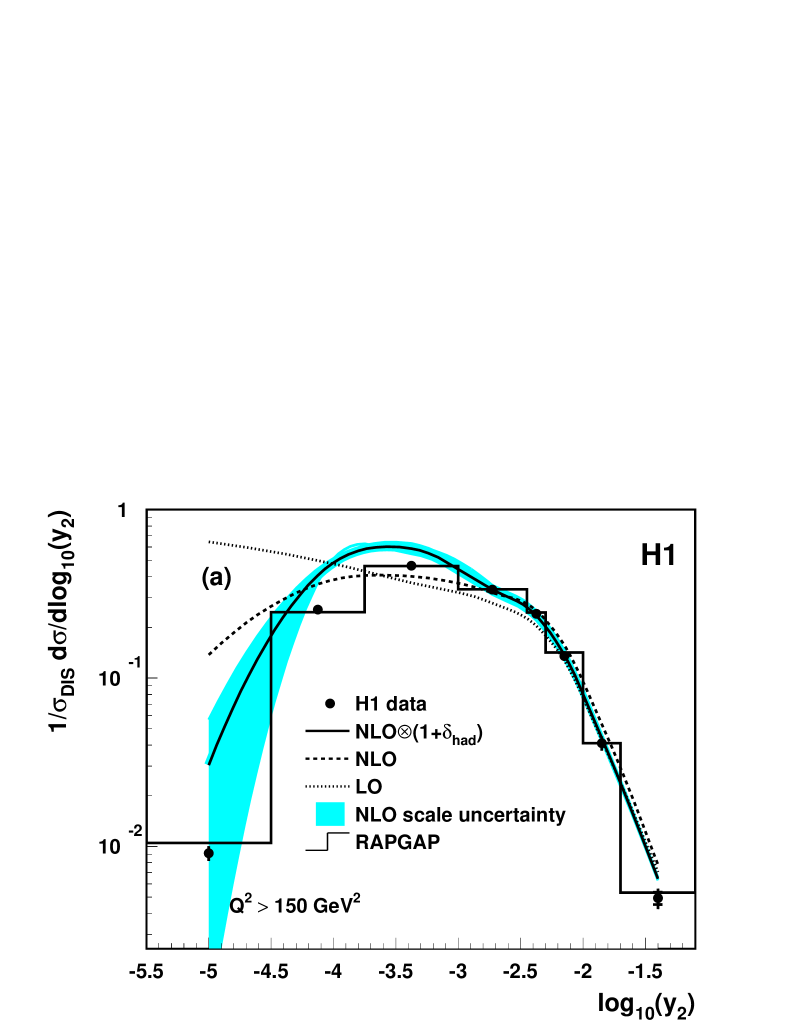
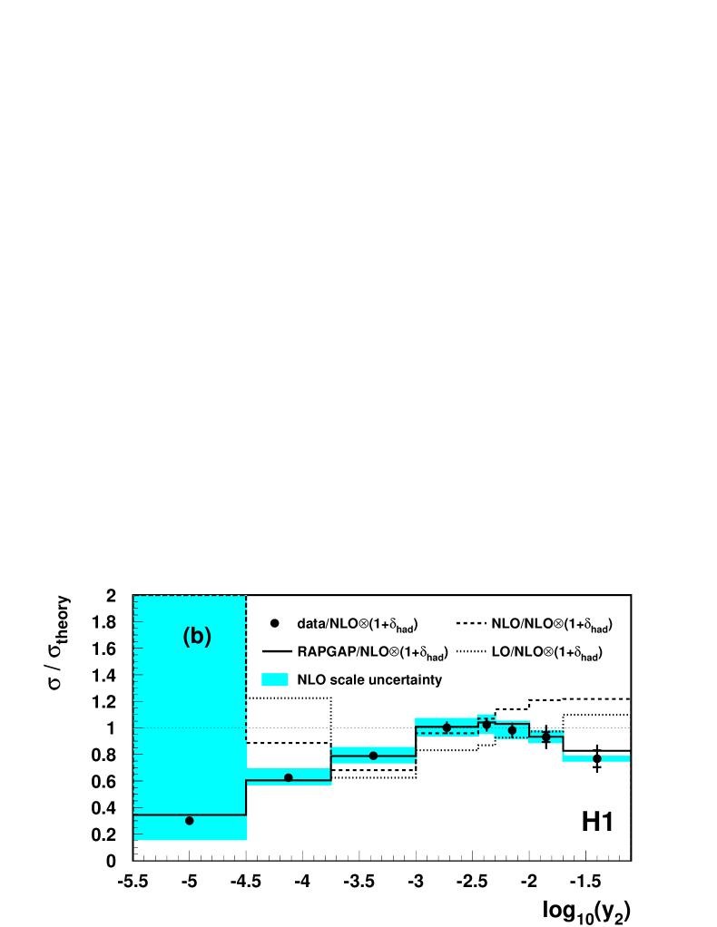
Figure 1: (a) Distribution of $y_{2}$ for $Q^{2}>150\,$GeV², determined with the modified Durham algorithm. The events satisfy $10^{\circ}<\theta_{\rm jet}<140^{\circ}$. Here, and in the following figures, the statistical errors are given by the inner error bars and the outer error bars correspond to the quadratic sum of the statistical and systematic errors. Also shown are perturbative QCD calculations in LO, in NLO with and without hadronization corrections, and the predictions of the QCD model RAPGAP. The shaded band shows the renormalization scale uncertainty of the NLO calculations, which is estimated here and below by varying $\mu_{R}$ in the range $Q/2$ to $2\,Q$.
(b) The ratios of the data and various predictions. The vertical error bars correspond to the uncertainty of the data only.

Figure 2: (a) Dijet event $\overline{E}_{T\,{\rm Breit}}$ distributions determined with the modified Durham algorithm in various $Q^{2}$ ranges. The dijet events satisfy $y_{2}>0.001$ and $10^{\circ}<\theta_{\rm jet}<140^{\circ}$. Also shown are perturbative QCD calculations in NLO with $\mu_{R}=Q$ and $\mu_{R}=\overline{E}_{T\,{\rm Breit}}$, and the predictions of the QCD model RAPGAP. The shaded band corresponds to the quadratic sum of the hadronization and renormalization scale uncertainties.
(b) The ratios of the data and various predictions. The vertical error bars correspond to the uncertainty of the data only.

Figure 3: Dijet event $\theta_{\textrm{fwd}}$ and $\theta_{\textrm{bwd}}$ distributions determined with the modified Durham algorithm in various $Q^{2}$ ranges. The dijet events satisfy $y_{2}>0.001$ and $10^{\circ}<\theta_{\rm jet}<140^{\circ}$. Also shown are perturbative QCD calculations in NLO and LO, the predictions of the QCD model RAPGAP, and a phase space calculation in arbitrary normalization. The shaded band corresponds to the quadratic sum of the hadronization and renormalization scale uncertainties.

Figure 4: Dijet event $z_{p}$ and $x_{p}$ distributions determined with the modified Durham algorithm in various $Q^{2}$ ranges. The dijet events satisfy $y_{2}>0.001$ and $10^{\circ}<\theta_{\rm jet}<140^{\circ}$. Also shown are perturbative QCD calculations in NLO with and without hadronization corrections, and the predictions of the QCD model RAPGAP. The shaded band corresponds to the quadratic sum of the hadronization and renormalization scale uncertainties. Note that the quark-induced contribution to the dijet cross section is close to 100% for $Q^{2}>5000$ GeV².

References

- [1] C. Adloff et al. [H1 Collaboration], Eur. Phys. J. C 21 (2001) 33 [hep-ex/0012053].
- [2] C. Adloff et al. [H1 Collaboration], Eur. Phys. J. C 19 (2001) 269 [hep-ex/0012052].
- [3] C. Adloff et al. [H1 Collaboration], Eur. Phys. J. C 13 (2000) 609 [hep-ex/9908059].
- [4] J. Breitweg et al. [ZEUS Collaboration], Phys. Lett. B 487 (2000) 53 [hep-ex/0005018].
- [5] J. Breitweg et al. [ZEUS Collaboration], Eur. Phys. J. C 11 (1999) 427 [hep-ex/9905032].
- [6] C. Adloff et al. [H1 Collaboration], Eur. Phys. J. C 19 (2001) 429 [hep-ex/0010016].
- [7] C. Adloff et al. [H1 Collaboration], Eur. Phys. J. C 19 (2001) 289 [hep-ex/0010054].
- [8] J. Breitweg et al. [ZEUS Collaboration], Phys. Lett. B 507 (2001) 70 [hep-ex/0102042].
- [9] R.P. Feynman, Photon-Hadron Interactions, Benjamin, New York (1972).
- [10] C. Adloff et al. [H1 Collaboration], Eur. Phys. J. C 14 (2000) 255 [Erratum-ibid. C 18 (2000) 417] [hep-ex/9912052].
- [11] J. Breitweg et al. [ZEUS Collaboration], Phys. Lett. B 421 (1998) 368 [hep-ex/9710027].
- [12] C. Adloff et al. [H1 Collaboration], Nucl. Phys. B 545 (1999) 3 [hep-ex/9901010].
- [13] J. Breitweg et al. [ZEUS Collaboration], Eur. Phys. J. C8 (1999) 367 [hep-ex/9804001].
- [14] N. H. Brook, T. Carli, E. Rodrigues, M. R. Sutton, N. Tobien and M. Weber, A comparison of deep inelastic scattering Monte Carlo event generators to HERA data, hep-ex/9912053.
- [15] H. Jung, Comput. Phys. Commun. 86 (1995) 147.
- [16] I. Abt et al. [H1 Collaboration], Nucl. Instrum. Meth. A 386 (1997) 310 and 348.
- [17] S. Catani, Y. L. Dokshitzer, M. Olsson, G. Turnock and B. R. Webber, Phys. Lett. B 269 (1991) 432.
- [18] J. G. Körner, E. Mirkes and G. A. Schuler, Int. J. Mod. Phys. A 4 (1989) 1781.
- [19] M. H. Seymour, Nucl. Phys. B 436 (1995) 443 [hep-ph/9410244].
- [20] E. Mirkes, Theory of jets in deep inelastic scattering, hep-ph/9711224.
- [21] L. Lönnblad, Comput. Phys. Commun. 71 (1992) 15.
- [22] G. Ingelman, A. Edin and J. Rathsman, Comput. Phys. Commun. 101 (1997) 108 [hep-ph/9605286].
- [23] G. A. Schuler and H. Spiesberger, DJANGO: The interface for the event generators HERACLES and LEPTO, Proceedings of the workshop Physics at HERA, Eds. W. Buchmüller and G. Ingelman, vol. 3 (1991) 1419.
-
[24]
V. Blobel,
DESY 84/118, Lectures given at 1984 CERN School of Computing,
Aiguablava, Spain, September 1984;
V. Blobel and E. Lohrmann, “Statistische und Numerische Methoden der Datenanalyse”, Teubner, 1998. 358 p, (Teubner-Studienbuecher: Physik), ISBN 3-519-03243-0 (in German). - [25] C. Adloff et al. [H1 Collaboration], Eur. Phys. J. C 5 (1998) 625 [hep-ex/9806028].
- [26] S. Catani and M. H. Seymour, Nucl. Phys. B 485 (1997) 291 [Erratum-ibid. B 510 (1997) 503] [hep-ph/9605323].
- [27] D. Graudenz and M. Weber, NLO Programs for DIS and Photoproduction: Report from Working Group 20, Proceedings of the workshop Monte Carlo Generators for HERA Physics, Eds. A. T. Doyle, G. Grindhammer, G. Ingelmann and H. Jung, DESY-PROC-1999-02 117.
- [28] C. Duprel, T. Hadig, N. Kauer and M. Wobisch, Comparison of next-to-leading order calculations for jet cross sections in deep-inelastic scattering, hep-ph/9910448.
- [29] G. J. McCance, NLO program comparison for event shapes, hep-ph/9912481.
- [30] V. Antonelli, M. Dasgupta and G. P. Salam, JHEP 0002 (2000) 001 [hep-ph/9912488].
- [31] H. L. Lai et al. [CTEQ Collaboration], Eur. Phys. J. C 12 (2000) 375 [hep-ph/9903282].
- [32] M. Bengtsson and T. Sjöstrand, Z. Phys. C 37 (1988) 465.
- [33] B. Andersson, G. Gustafson, G. Ingelman and T. Sjöstrand, Phys. Rept. 97 (1983) 31.
- [34] T. Sjöstrand and M. Bengtsson, Comput. Phys. Commun. 43 (1987) 367.
- [35] H. L. Lai et al., Phys. Rev. D 55 (1997) 1280 [hep-ph/9606399].