Correlations in the
Charged-Particle Multiplicity Distribution

Supervisor:                     Prof. Dr. E.W. Kittel

Co-supervisor:                Dr. W.J. Metzger

Manuscript Committee: Prof. Dr. A. Giovannini (University of Torino)

Prof. Dr. E. Longo (University of Roma)

Dr. J. Field (University of Geneva)

The work described in this thesis is part of the research programme of the “Nationaal Instituut voor Kernfysica en Hoge-Energie Fysica” (NIKHEF). The author was financially supported by the “Stichtig voor Fundamenteel Onderzoek der Materie” (FOM).

ISBN 90-9015317-9

La chose la plus difficile n’est pas de s’attaquer à une de ces

grandes questions insolubles mais bien d’adresser à quelqu’un

un petit mot délicat où tout est dit et rien.

E.M. Cioran

Introduction

What can we learn about the dynamics of particle production in collision by just looking at the number of particles produced in the final state ?

This is the main question which is addressed in this thesis.

It is remarkable that the study of a static variable, such as the number of particles found in the final state, might reveal anything about the chain of processes which have occurred in the early stage of the reaction.

By analogy, one can imagine an extra-terrestrial being wanting to understand Humanity from outside the Earth by using a giant telescope and looking at the distribution of light density at the surface of the Earth, from the behavior of this light density trying to access information about Humanity and its evolution.

What he would see is that the light density is not uniform, that in some areas there is practically nothing, while at other places huge clusters of light density occur. He might also see that large light density areas are connected to middle range light density areas by thin light density lines. He would then find an obvious hierarchy in the distribution of these lights. In order to understand the mechanism which governs the apparition and the evolution of the light density, he would try to understand how all these lights are connected to each other. Therefore, he would study the correlations between these light densities.

He would certainly not understand the human spirit, but he might be able to understand some important points, both about the present and the past of Humanity and also about its evolution. Quickly, he would understand that these areas of high light densities have a “capital” importance for the whole light density distribution and that they, somehow, govern the evolution of smaller light density areas. He may argue that this importance dates back to some early stage in Humanity evolution when the light population was smaller and that by some iterative migration waves, the light population has increased. He may even argue about the reason why these areas have been favored above the others. He may decompose the dynamics of this light density evolution in this area into two stages, a first stage dating back to the origin of the apparition of the light in this area and a second one coming from the fact that the growing importance of this area itself might have led this area to grow in importance (and in light density) even faster. He may not realize that Humanity (at least what he thinks Humanity is) has anything to do with some living creatures crawling at the surface of Earth. However, he will always be able to manage some understanding concerning the main points in the evolution of Humanity.

Luckily, particle physics is rather well understood (so we think). Main stream theories collected under the common name of Standard Model of particle physics describe in great detail many aspects of particle physics. Therefore, we should be able to learn more about the dynamics of particle production than our E.T. scientist can about Humanity.

The main-stream theory of primary concern in this thesis is is Quantum ChromoDynamics (QCD), the theory of the strong interaction which insures at its smallest scale the cohesion of matter, explaining the way in which quarks and gluons are bound together within protons and neutrons, which are themselves held within the atomic nucleus. QCD was born in the 1970’s. So it is still a rather young theory and many questions have yet to be answered. One of them concerns the evolution of partons into hadrons. Currently, no theory is able to describe the entire process.

This thesis describes research that takes place at the interface between soft and hard QCD (the sector of QCD which describes hadrons and that which describes partons, respectively) and it is intended to help to understand the general picture of the evolution of partons to hadrons.

By studying the charged-particle multiplicity distribution, we are able to access the dynamics of the process. The way partons evolve into hadrons leaves footprints in the charged-particle multiplicity distribution of the final state. These footprints are the correlations which exist between the particles. By studying these correlations, one might be able to pinpoint the various processes responsible for the particles we record in our detector.

Therefore, to give a short answer to the question asked at the beginning of this introduction, the study of the charged-particle multiplicity distribution will help us to better understand the chain of processes and their hierarchical importance in the production of final state particles.

The layout of the thesis is organized as follows: In Chapter 1, a short theoretical introduction to multiparticle production is given. LEP and the L3 detector, the source of the data used in our analysis, are described in Chapter 2. In Chapter 3, the selection, , the necessary step to isolate a pure sample of hadronic $\mathrm{Z}^{0}$ decays, is described. The measurement of our main variable, the charged-particle multiplicity, is described in Chapter 4. The inclusive charged-particle spectrum is measured in Chapter 5. Chapter 6 is the first chapter dedicated to the study of the shape of the charged-particle multiplicity distribution. In this chapter the study is limited to the full event sample and to a comparison with theoretical predictions. In Chapter 7, the shape of the jet multiplicity distribution is studied in order to enable direct comparison with QCD and jets obtained at perturbative energy scales. In Chapter 8, the charged-particle multiplicity distribution of the full sample is subdivided into that of 2-jet and 3-jet samples in order to compare to phenomenological models. The charged-particle multiplicity distribution is also studied in restricted rapidity intervals in Chapter 9. Finally, the conclusions are summarized.

Chapter 1 Theory

We present in this chapter a short introduction to the theoretical knowledge and understanding of the processes occurring during an collision and responsible for the properties of the observables such as the charged-particle multiplicity distribution and reduced momentum distribution studied in this thesis.

1.1 Multiparticle production in collisions

Multiparticle production is studied in a wide range of processes, from heavy-ion to interactions. Unlike other types of collisions, the interaction has the advantage of offering a clean framework for this study. Only one collision per bunch crossing occurs, furthermore all the available center-of-mass energy is used in the interaction. Electrons and positrons being point-like and massless particles, and interacting only via the Electroweak interaction, their interaction is well understood and described by the Standard Model.

At the center-of-mass energy of $\sqrt{s}=91.2~{}\GeV{}$, at the $\mathrm{Z}^{0}$ resonance, the interaction is dominated by the production of a quark and anti-quark pair (and hence of hadrons) via the formation of a $\mathrm{Z}^{0}$ boson. The cross section of this process is about $69.9\%$ [1] of the total cross section. From a theoretical point of view, the process $\mathrm{e^{+}}\mathrm{e^{-}}\longrightarrow\text{hadrons}$ is understood as a succession of phases, each of them being described by a different theory. The main phases in the evolution of an multi-hadronic event are shown in Fig. 1.1 together with its structure.

The electroweak phase

The first phase of the process concerns the collision itself. The electron-positron pair annihilates into a virtual photon or a $\mathrm{Z}^{0}$ boson. This phenomenon may be accompanied by the emission of photons (initial-state radiation) prior to the annihilation. Following its creation, the vector boson decays into a quark-antiquark (  ) pair. As for the annihilation, the creation of the fermion pair may be accompanied by the emission of one or more photons (final-state radiation). Both initial- and final-state radiation affect the system by reducing the energy available for hadron production. However, both initial- and final-state radiations are not very common at the energy of the $\mathrm{Z}^{0}$. All these phenomena are described in the framework of the very successful electroweak model.

The perturbative QCD phase

From the    pair created in the previous phase, a large number of particles are produced in the final-state in a very characteristic jet structure, as seen in Fig. 1.2 for a 3-jet event as it appears in the L3 detector. Quantum ChromoDynamics (QCD) gives, in principle, a description and explanation for both the large number of particles produced in the final-state and its jet structure.

HADRONIZATION

DECAY

Figure 1.1: Schematic representation of a hadronic event.

In Quantum ChromoDynamics, multiparticle production arises from the interactions of quarks and gluons [2]. Because of their properties, these interactions are responsible for the creation of additional quark-antiquark pairs and gluons ( partons) in a cascade process near the direction of the primary partons ( the initial quarks and gluons), thus giving this typical jet structure to the events. Ultimately, hadronization gives birth to a large number of hadrons arranged into jets.

Two approaches may be used to described the production of partons.

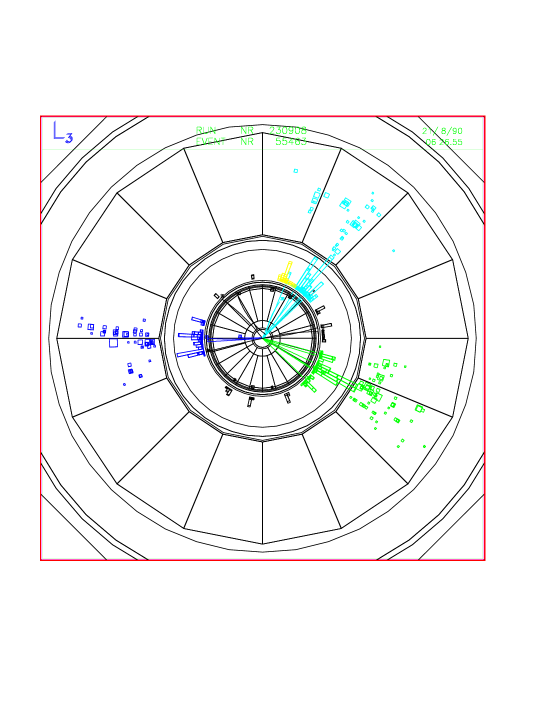
Figure 1.2: A hadronic event as seen in the L3 detector.

The first one, known as the matrix element method (M.E.), consists of performing the exact calculation perturbatively at each order of the strong coupling constant $\alpha_{\text{s}}$, taking into account all Feynman diagrams. Unfortunately, the difficulty increases sharply with the order considered and such a calculation has not yet been performed to more than the second order in $\alpha_{\text{s}}$. Therefore, this method cannot account for more than 4 partons in the final-state.

Instead of using the exact calculation, the second approach, known as the parton shower approach, attempts to reproduce the cascade process responsible for the jet structure of the event. This is achieved by making iterative use of the three basic branchings allowed by QCD, $\text{q}\rightarrow\text{qg}$, $\text{g}\rightarrow\text{q}\bar{\text{q}}$ and $\text{g}\rightarrow\text{gg}$. The probabilities governing the occurrence of these branchings are obtained from the Dokshitzer-Gribov-Lipatov-Altarelli-Parisi (DGLAP) evolution equations [3] as a function of the transverse momentum of the partons. These equations are calculated using perturbative theory, in the Leading-Logarithm Approximation (LLA) by taking into account in the expansion only the leading terms in $(\alpha_{\text{s}}\ln^{2}(s))^{n}$, the so-called leading logarithms. Extensions to this model such as Double LLA (DLLA), Modified LLA (MLLA), Next to LLA (NLLA) and even Next to Next to LLA (NNLLA) have been investigated. These approximations take into account subleading terms ignored in the LLA, which allows them to account for effects such as gluon coherence (responsible for angular ordering which causes each subsequent gluon to be radiated within a smaller cone than its parent) and which better incorporate energy-momentum conservation.

The parton shower approach makes use of the running property of $\alpha_{\text{s}}$, which decreases to 0 at large energy scales (asymptotic freedom), enabling perturbative calculations to be carried out. On the other hand, at small energy scales $\alpha_{\text{s}}$ becomes large, thus forbidding the use a of power expansion in $\alpha_{\text{s}}$. This imposes a limit on the perturbative calculation of the development in the cascade process to energy scales larger than about 1 , defining what is often called the perturbative region (illustrated in Fig 1.1) of QCD.

The non-perturbative phase

At small energy scales, where $\alpha_{\text{s}}$ is large, the use of perturbation theory can not be justified. Therefore, this phase is called the non-perturbative phase.

This third phase may itself be decomposed into two parts. In the first part, the hadronization, colored partons fragment into colorless hadrons. In the second part, these hadrons, which are for the most part unstable, decay into the stable particles which constitute the final-state particles observed in the detector (Fig. 1.2).

In order to make final-state particles accessible to theoretical predictions, two approaches are often used:

The Analytical Perturbative Approach widely used to extrapolate analytical QCD predictions to final-state particles assumes Local Parton-Hadron Duality (LPHD) [4]. The LPHD hypothesis relies on the idea of pre-confinement [5], which implies that before hadronization colored partons are locally (in phase space) grouped into colorless clusters keeping the main properties of the partonic final-state. Consequently, the hadronic final state can be directly compared to the analytical QCD predictions for partons. The use of this method is limited to infrared safe variables, which are, in principle, not distorted by the hadronization phase. For such variables, partons and hadrons differ by only a proportionality factor,

$$\text{q}_{\text{hadron}}\propto\text{q}_{\text{parton}}.$$ (1.1)

This method does not describe the final-state particles, but offers a rather good description of the behavior of some of the quantities characterizing the final-state particles, such as the energy evolution of the average number of charged particles and of their momentum.

Since the description of the final-state particles cannot be accessed analytically, a second approach is to use phenomenological models. Such models can provide a more complete description of the final-state. The various models available to describe the hadronization are Monte Carlo based models. They are described in the following section.

For completeness, we also mention lattice QCD [6], which has enjoyed large success in describing non-perturbative effects, but which has not yet been applied to hadronization.

1.2 QCD generators

Monte Carlo generators are essential for our study. They are able to generate a complete particle final-state which can then be compared to the final-state particles resulting from the interaction, from which the quantities relevant to our analysis are extracted.

Each event is generated independently of the others. For each event, the whole chain of processes leading to the hadronic final-state is generated. Each property, such as quark flavor, particle directions, energy they carry, the way they decay, is randomly generated according to its probability of occurrence determined by the physics of the process. The generator also takes into account all the constraints and limitations imposed by the dynamics and the kinematics imposed by the whole chain of processes.

The main Monte Carlo models used to simulate hadronic Z decays in this thesis are the JETSET 7.4 [7], HERWIG 5.9 [8] and ARIADNE 4.08 [9, 10] Monte Carlo programs.

The generation of hadronic events proceeds in two main stages. The parton generation, which implements perturbative QCD to produce partons, and the fragmentation, which treats in a phenomenological way the hadronization as well as the decay of the particles. The main approaches used in the Monte Carlo generators to describe these stages and their specification are reviewed in the following two sub-sections. Furthermore, these models incorporate special treatment to take into account the weak decay of heavy quarks.

1.2.1 Parton generation

Both Matrix Element and Parton Shower QCD approaches to parton generation have been implemented in Monte Carlo generators.

The Matrix Element approach

The Matrix Element approach is found as an option in JETSET. It implements matrix element calculations up to $\mathcal{O}(\alpha_{\text{s}}^{2})$ allowing to choose between a maximum of 2, 3 or 4 partons in the final-state.

The parton shower approach

Parton shower models are implemented in JETSET, HERWIG, and ARIADNE. An important advantage over the analytical perturbative QCD calculations is that full energy-momentum conservation is imposed at each branching in the Monte Carlo models. Thus, Monte Carlo parton shower models implement, intrinsically, some higher-order corrections ignored by their analytical counterparts.

The JETSET parton shower implementation generates partons according to the LLA framework. This model does not take into account subleading effects responsible for gluon interference, but an option exists to force it by requiring angular ordering explicitly. This makes the parton shower equivalent to an MLLA parton shower.

HERWIG and ARIADNE with its color dipole cascade [11] use different approaches for their parton shower. Both of them take intrinsically into account coherence effects, which also makes them equivalent to a MLLA parton shower.

1.2.2 Fragmentation models

Since hadronization cannot be described analytically, phenomenological models are used. There are mainly three different models, the Lund string model [12] implemented in JETSET, which is the most popular (and also the most successful in describing the data), the cluster model [13] implemented in the HERWIG generator, and the independent fragmentation model [14, 15], an older model still implemented in JETSET as an option.

Independent fragmentation model

In the independent fragmentation model, each final-state parton fragments independently from the others. It fragments into a mesonic cascade until no energy is left to allow further splitting.

This model, whose origin dates back to the beginning of the seventies, gives only a poor description of the data. It has been supplanted by more recent models, such as the string and cluster models discussed below. Therefore, it is practically not used anymore. Nevertheless, since all partons fragment independently, we will find it useful as a toy model to investigate the origin of certain correlations. It may help understanding part of the effects brought in by the hadronization. But, because of the very approximative description of the hadronization, we cannot make detailed comparisons of this model to the data.

Cluster fragmentation model

The cluster fragmentation model is an implementation of the pre-confinement property, from which originates the LPHD hypothesis. It assumes that after the parton shower, partons are locally aggregated into colorless hadrons. Therefore, in the cluster model, all the gluons resulting from the parton shower are split into light (u or d) quark-antiquark or diquark-antidiquark pairs. These clusters are then fragmented into hadrons.

The Lund string model

The Lund string model is certainly the most popular and successful fragmentation model. In the string model, a color string is stretched between quark and anti-quark. The quark and antiquark moving apart along this string lose energy. This causes the string to break into two new quark-antiquark systems, resulting in two new strings which will break up similarly. The breaking process eventually stops when the mass of the string pieces has fallen to the hadron mass. These string pieces form the hadrons. In this model, gluons are treated as kinks on the string.

This model appears to give a good description of the data in the final-state.

1.2.3 Final-state particles

Most of the hadrons produced by the fragmentation models described above are unstable and must decay into stable particles. The quantitative knowledge we have about decays is mainly experimental. Therefore, at this stage, most of the masses and branching ratios governing the decays of these particles are taken from experimental results, with subsequent tuning in order to optimize the description of the data by the Monte Carlo models.

Furthermore, all these Monte Carlo models have adjustable parameters and switches, whose values are chosen in order to ensure a good description of the experimental data.

1.3 $\xi$ spectrum

The single-particle inclusive momentum spectrum in $\xi=-\ln(x)$, where $x$ is the scaled momentum ( $x=2p/\sqrt{s}$, where $p$ is the particle momentum and $\sqrt{s}$ the center of mass energy), is very sensitive to soft gluon radiation. Its description, therefore, constitutes an important test of perturbative QCD, in particular of the MLLA, which takes into account subleading terms introducing soft gluon radiation corrections. These corrections take into account color coherence, which leads to soft gluon suppression at large angles and hence to hadron depletion at low momentum. This effect is also characterized by a strong angular ordering of gluon production, each gluon being emitted with a smaller angle than its parent. The effect of color coherence can be seen in the $\xi$ distribution, where it results in the so-called MLLA hump-backed plateau [16, 17] shape of the $\xi$ distribution.

In the DLLA approximation which contains the premise of the color coherence effect [18] (and only a rough estimate of the angular ordering), the $\xi$ spectrum is described by a Gaussian. Applying a next to leading order correction to the DLLA prediction, corresponding to MLLA, causes the $\xi$ distribution to deviate from the Gaussian shape, becoming a platykurtic shape [19], which has the appearance of a skewed and flattened Gaussian. This is also characterized by a shift to lower momentum of the peak position, $\xi^{\star}$, of the $\xi$ distribution.

Under the LPHD assumption, this behavior is not distorted by hadronization and is therefore identical for partons and hadrons.

Furthermore, as a confirmation of the MLLA (or as a need to take into account angular ordering), the evolution of the peak position $\xi$ with the center-of-mass energy has been found to be described by the MLLA, while the DLA has failed to describe it [20, 21, 22, 23, 24].

1.4 The charged-particle multiplicity distribution

One of the most fundamental observables in any high-energy collision process is the total number of particles produced in the final-state and by extension the number of charged particles which detection are easier. Even if this is only a global measure of the characteristics of the final-state, it is an important parameter in the understanding of hadron production. Independent emission of single particles leads to a Poissonian multiplicity distribution. Deviations from the Poissonian shape reveal correlations [25]. Therefore, these correlations are the signatures of the mechanisms involved from the early stage of the interaction with the appearance of the primary partons to the production of the particles in the final-state.

Using appropriate tools, it is, therefore, possible to extract information about the dynamics of particle production from the shape of the charged-particle multiplicity distribution.

The usual way of studying the charged-particle multiplicity distribution and its shape, is to calculate its moments. General characteristics of the charged-particle multiplicity distribution are obtained using low-order moments, such as the mean, $\mu_{1}$, the dispersion, $D$, which estimates the width of the distribution, the skewness, $S$, which measures how symmetric the distribution is, and the kurtosis, $K$, which measures how sharply peaked the distribution is. With $P(n)$ the charged-particle multiplicity distribution and $\langle q\rangle$ symbolizing the average of a quantity $q$, these moments are defined by

$$\mu_{1}=\langle n\rangle=\overset{\infty}{\underset{n=1}{\sum}}nP(n)\text{ , }D=\sqrt{\langle(n-\mu_{1})^{2}\rangle}\text{ , }S=\frac{\langle(n-\mu_{1})^{3}\rangle}{D^{3}}\text{ , }K=\frac{\langle(n-\mu_{1})^{4}\rangle}{D^{4}}-3.$$ (1.2)

However, these moments only give information about the main properties of the distribution. A more detailed study of the charged-particle multiplicity distribution and of its shape, and in particular the study of correlations (and hence, the study of particle production) requires high-order moments [25]. A way, often used, of studying the correlations between particles in the charged-particle multiplicity distribution is to measure the normalized factorial moments of order $q$,

$$F_{q}=\frac{\overset{\infty}{\underset{n=q}{\sum}}n(n-1)....(n-q+1)P(n)}{\left(\overset{\infty}{\underset{n=1}{\sum}}nP(n)\right)^{q}}.$$ (1.3)

The factorial moment of order $q$ corresponds to an integral over the $q$-particle density and reflects correlations in particle production. If particles are produced independently the multiplicity distribution is Poissonian (see Fig. 1.3(a)), and all the $F_{q}$ are equal to unity. If the particles are correlated, the distribution is broader than Poisson and the $F_{q}$ are larger than unity (see example of the negative binomial distribution in Fig. 1.3(a)). In the opposite case, if the particles are anti-correlated, the distribution is narrower than Poisson, and the $F_{q}$ are smaller than unity. Two examples of $F_{q}$ plotted as a function of the order $q$ are shown in Fig. 1.3(b), for distributions such as the Poisson distribution (no correlation) and for a negative binomial distribution (positive correlation).

However, with the $F_{q}$ we only access the sum of all correlations existing among $q$ or fewer particles. It is a combination which takes into account all possible correlations between any number of particles, smaller or equal to the order $q$. Therefore, one can access the genuine $q$-particle correlation by the use the normalized cumulant factorial moments, $K_{q}$, which are obtained from the normalized factorial moments by

$$K_{q}=F_{q}-\overset{q-1}{\underset{m=1}{\sum}}\frac{(q-1)!}{m!(q-m-1)!}K_{q-m}F_{m}.$$ (1.4)

These $K_{q}$ correspond to the phase-space integral over the genuine $q$-particle correlation. If the particles result from independent emission (Poissonian behavior), the $K_{q}$ are equal to 0. The $K_{q}$ are positive if the particles are correlated and negative if the particles are anti-correlated. As examples, the $K_{q}$ plotted versus the order $q$ are given in Fig. 1.4(a), for the Poisson (no correlation) and for the negative binomial distribution (positive correlation) and also for the experimental charged-particle multiplicity distribution, which will be studied in details in chapter 4.

Since $F_{q}$ and $|K_{q}|$ both increase with the order $q$, it is useful to define the ratio $H_{q}$:

$$H_{q}=\frac{K_{q}}{F_{q}}=1-\overset{q-1}{\underset{m=1}{\sum}}\frac{(q-1)!}{m!(q-m-1)!}H_{q-m}\frac{F_{m}F_{q-m}}{F_{q}}.$$ (1.5)

The $H_{q}$ moments reflect the genuine $q$-particle correlation integrals relative to the density integrals. They characterize the weight of the genuine $q$-particle correlations with respect to the whole spectrum of correlations between $q$ particles. Furthermore, the $H_{q}$ moments have the advantage over the $F_{q}$ and $K_{q}$ of being of the same order of magnitude for a large range of $q$. Examples of $H_{q}$ plotted versus the order $q$ are given in Fig. 1.4(b), for the Poisson and the negative binomial distribution, together with the one measured from the experimental charged-particle multiplicity distribution.

Figure 1.3: Poisson and negative binomial distributions , together with the charged-particle multiplicity distribution of the experimental data (a). $F_{q}$ vs $q$ obtained from Poisson and negative binomial distributions, together with the $F_{q}$ measured from the experimental data (b).

Figure 1.4: $K_{q}$ vs $q$ (a) and $H_{q}$ vs $q$ (b), obtained from Poisson and negative binomial distributions, together with those measured from the experimental data.

More astonishing than from Poisson and negative binomial are the $H_{q}$ moments obtained from the experimental charged-particle multiplicity distributions (Fig. 1.4(b)), exhibiting an oscillatory behavior when plotted versus the order $q$. Furthermore, the same qualitative oscillatory behavior has been observed not only in collisions, but also in hadron-hadron, hadron-ion and even ion-ion collisions [26, 27].

The usual way to interpret this oscillatory behavior is to refer to perturbative QCD, which provides us with calculations for the $H_{q}$ of the parton multiplicity distribution [28, 26]. Under the local parton-hadron duality hypothesis, which assumes that the shape of the parton multiplicity distribution is not distorted by hadronization, perturbative QCD prediction may be valid for hadrons, thereby allowing the extension of perturbative QCD predictions to the shape of the charged-particle multiplicity distribution.

However, this result can also be interpreted in a more phenomenological way by viewing the shape of the charged-particle multiplicity distribution as the result of the fact that different types of events, such as 2-jet or 3-jets events, compose the total charged-particle multiplicity distribution [29].

1.4.1 $H_{q}$ moments and analytical QCD predictions

Since the evolution equations of QCD can be described in probabilistic terms using generating functions, it is, in principle, possible to describe analytically the parton multiplicity distribution. Nevertheless, even an approximate solution to this equation cannot be obtained easily. However, it has turned out to be a relatively easy problem to solve for the moments of the multiplicity distribution. Therefore, the $H_{q}$ moments have been calculated up to the next-to-next-to-leading logarithm approximation [28]. The expected behavior of $H_{q}$ for various approximations is qualitatively plotted as a function of $q$ in Fig. 1.5.

Figure 1.5: Qualitative behavior of $H_{q}$ vs. $q$ for various perturbative QCD approximations.

• For the Double Leading Logarithm Approximation (DLLA), $H_{q}$ decreases to 0 as $q^{-2}$.

• For the Modified Leading Logarithm Approximation (MLLA), $H_{q}$ decreases to a negative minimum at $q=5$, and then rises to approach 0 asymptotically.

• For the Next-to-Leading Logarithm Approximation (NLLA), $H_{q}$ decreases to a positive minimum at $q=5$ and then increases to a positive constant value for large moment rank.

• For the Next-to-Next to Leading Logarithm Approximation (NNLLA), $H_{q}$ decreases to a negative first minimum for $q=5$, and for $q>5$, $H_{q}$ shows quasi-oscillations about 0.

The main difference between all these approximations lies in how energy momentum conservation is incorporated. The most accurate treatment is given by the NNLLA.

Similar behaviors as those predcited are expected for the charged-particle multiplicity distribution under the Local Parton-Hadron Duality hypothesis. The oscillatory behavior observed in Fig. 1.4(b) is often interpretated as a confirmation of NNLLA and LPHD.

1.4.2 Phenomenological approaches

However, the $H_{q}$ oscillatory behavior may also be interpreted in a more phenomenological way making use of different classes of events, which themselves do not necessarly have $H_{q}$ oscillations.

These approaches are based on the idea that the main features of the shape of the charged-particle multiplicity distribution and the oscillatory behavior of the $H_{q}$ could originate from the superposition of different types of events, as the 2-jet and 3-jet events [29] or the light- and b-quark samples [30], which compose the full sample.

Under this hypothesis, assuming we are able to describe individually the charged-particle multiplicity distributions of these different types of events using suitable parametrizations, the charged-particle multiplicity distribution of the full sample could then be described by a weighted sum of all the individual parametrizations, the weight being related to the rates of the various type of events.

If the full sample can be resolved into various classes of events, we can express its charged-particle multiplicity distribution as a sum of the various contributions:

$$P(n)=R_{\alpha}P_{\alpha}(n)+R_{\beta}P_{\beta}(n)+R_{\gamma}P_{\gamma}(n)+\ldots,$$ (1.6)

where the $P_{\alpha}(n)$, $P_{\beta}(n)$ and $P_{\gamma}(n)$ are the charged-particle multiplicity distributions of events of type $\alpha,\beta\text{ and }\gamma$, while $R_{\alpha,\beta,\gamma}$ are their respective rates.

Assuming these charged-particle multiplicity distributions are described by the parametrizations $f_{\alpha}(n)$, $f_{\beta}(n)$ and $f_{\gamma}(n)$, the charged-particle multiplicity distribution of the full sample, $P(n)$, will then be described by $f_{\text{full}}(n)$, the weighted sum of all the parametrizations:

$$f_{\text{full}}(n)=R_{\alpha}f_{\alpha}(n)+R_{\beta}f_{\beta}(n)+R_{\gamma}f_{\gamma}(n)+\ldots.$$ (1.7)

In our analysis, we make the choice to use the Negative Binomial Distribution (NBD) as parametrization. The NBD has been already used, with more or less success, in many types of interactions to describe their charged-particle multiplicity distributions [31]. The use of the NBD, as for the phenomenological approach, in multiparticle dynamics is intimately associated to the clan concept [32, 33]. This concept was used to explain the apparent NBD behavior of the multiplicity distribution observed in many experiments, processes and energies in both full and restricted phase space. A clan is defined as a group of particles originating from the same parent particle [34]. While the particle distribution within a clan is assumed to be logarithmic, its composition with other clans (which are assumed to be independent of each other) leads to the NBD.

In annihilation at the $\mathrm{Z}^{0}$ energy, it has been found that the charged-particle multiplicity distribution cannot be described by a single NBD [35]. Therefore, it is interesting to try combinations of NBDs [29, 30]. The NBD parametrization is given by

$$f^{\text{NB}}(n,\langle n\rangle,k)=\frac{\Gamma(k+n)}{\Gamma(n+1)\Gamma(k)}\left(\frac{k}{\langle n\rangle+k}\right)^{k}\left(\frac{\langle n\rangle}{\langle n\rangle+k}\right)^{n},$$ (1.8)

where $\langle n\rangle$ is the mean of the distribution and $k$ is given by

$$\frac{D^{2}}{\langle n\rangle^{2}}=\frac{1}{\langle n\rangle}+\frac{1}{k},$$ (1.9)

$D$ being the dispersion. Using the means and dispersions from the experimental distributions, we can then have fully constrained parametrizations of the charged-particle multiplicity distributions of the various classes of events and subsequently of the full sample. In Chapter 8, several phenomenological approaches based on this concept will be examined and confronted with the experiment.

Chapter 2 Experimental apparatus

2.1 The LEP collider at CERN

Located near Geneva, between the Alps and the Jura, the Large Electron Positron collider, LEP (Fig. 2.2), commissioned and operated by CERN, straddles the French-Swiss border at an average depth of about 100 meters.

LEP, with a circumference of 27 km, is the largest (electron-positron) collider built so far. It was designed to store and accelerate electrons and positrons, which it did up to the energy of $104.5\GeV$ per beam reached during the last data taking period in 2000. The electrons and positrons are produced and accelerated up to $20\GeV$ by lower energy CERN accelerators. They are then injected into LEP and concentrated into equidistant bunches circulating in opposite direction. Finally, they are accelerated to their final energy. Once they have reached that energy, they are allowed to collide at four of the eight equidistant crossing points. At these four crossing points are positioned the four LEP experiments: ALEPH, OPAL, DELPHI and in particular L3, the source of the data used in this analysis.

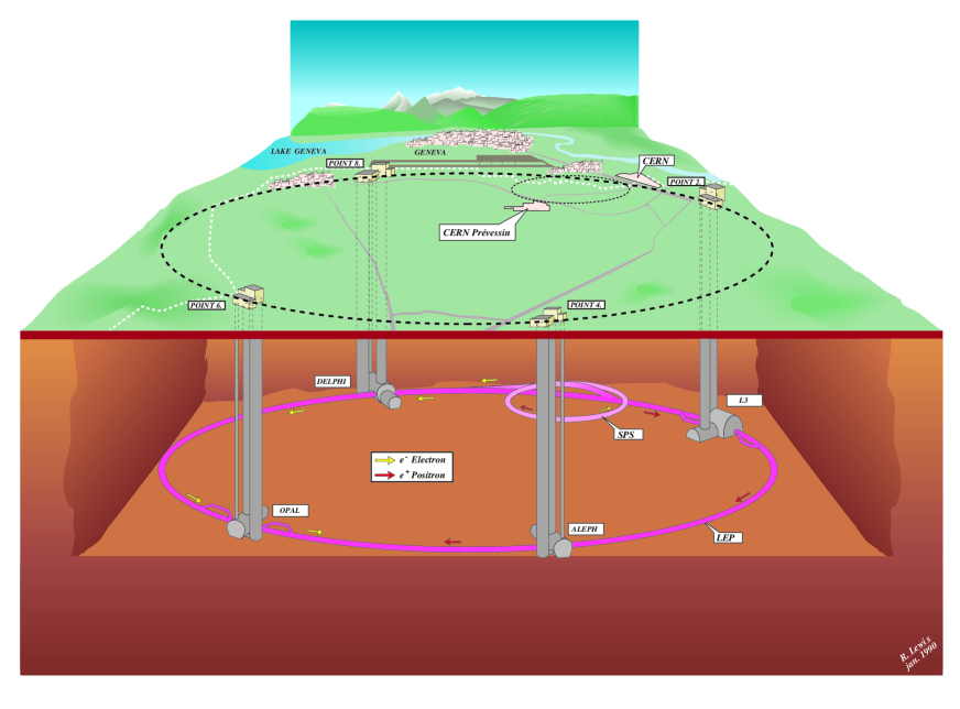
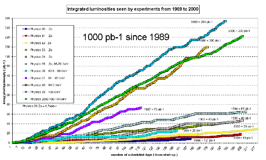
Figure 2.1: Underground and aerial view of LEP and its surrounding area.

Figure 2.2: Integrated luminosity per LEP experiment.

During more than 10 years, LEP has exploited to its limit the current technology and design. The limitation for such a design is synchrotron radiation, which depends on the curvature of the collider and on the energy of the electron or positron beam. Higher energies than those reached by LEP would require more power to replace the energy radiated or even larger rings to reduce the curvature and hence the synchrotron radiation, both of which are expensive. Therefore, the future of electron-positron colliding machines lies in new technologies which explore linear collider design ( TESLA at DESY, CLIC at CERN, JLC in Japan and NLC in the U.S., where already the first collider of this kind, the SLC at SLAC, has successfully fulfilled its goals).

The LEP collider was in operation from August 1989 to November 2000. A summary of the whole LEP activity is given in Fig. 2.2 in terms of integrated luminosities per LEP experiment. From 1989 to 1995, the LEP I period, its working energy was around the $\mathrm{Z}^{0}$ mass, near $91.2\GeV$. This period was dedicated to the extensive study of the parameters of the Z boson. About 4 million $\mathrm{Z}^{0}$ events were collected during this period. During 1995, a major upgrade took place in order to increase the LEP working energy, to enable the production of $\text{W}^{\pm}$ bosons and to continue the search for Higgs bosons and for supersymmetry already started at LEP I. During this new era, called LEP II, the LEP energy was gradually increased up to $209\GeV$ in 2000. The year 2000 also saw the report by ALEPH and L3 of events compatible with a Higgs signal. However, too few events were reported to confirm a discovery, but too many to be rejected as a simple statistical fluctuation. Nevertheless, this was the motivation for an extension of the data taking period from September to November 2000. However the additional data collected during this period did not settle the issue. It was finally decided to definitely close LEP on this status quo, leaving this question unanswered, but open to the higher energy collider TEVATRON at FNAL as well as to the next generation of colliders and, in particular, for the Large Hadron Collider (LHC), whose construction has already started in the LEP tunnel.

2.2 The L3 detector

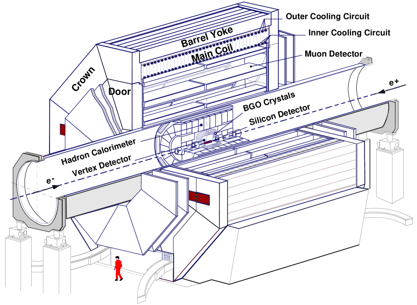
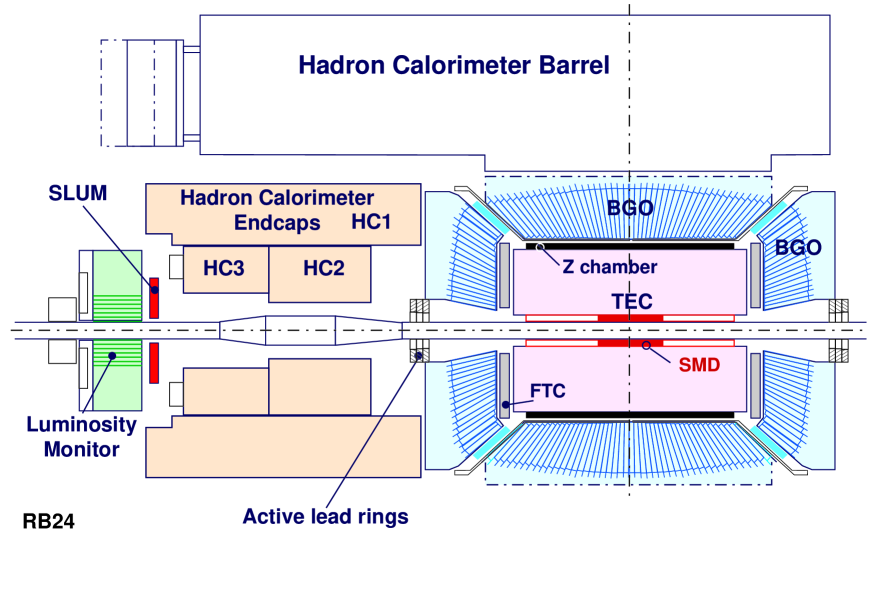
Figure 2.3: Perspective view of the L3 detector.

Figure 2.4: Longitudinal view of the inner part of the L3 detector.

Fig. 2.4 shows a perspective view of the L3 detector. The basic orientation of the detector is defined from the interaction point (at the center of the detector), which is the origin of the coordinate system in which the analysis takes place. Using the interaction point as origin, we define the coordinate system in the following way. The $x$ axis is perpendicular to the beam pipe, toward the center of LEP ring, the $y$ axis perpendicular to the beam pipe, pointing towards the top of the detector, the $z$ axis along the beam pipe, in the direction of the electron beam. It is also useful to define this system in spherical coordinates, where $r$ is the distance taken from the origin, $\theta$ is the angle between $\vec{r}$ and the $z$ axis, and $\phi$ the angle between the $x$ axis and $\vec{s}$, the projection of $\vec{r}$ onto the $xy$ plane.

The L3 detector is, in fact, composed of several subdetectors, which are fully described in [36]. These subdetectors are all inside a huge octagonal iron magnet of $12\text{m}\times 12\text{m}\times 12\text{m}$, which delivers a uniform magnetic field of 0.5 T along the $z$ axis.

From the magnet wall to the interaction point, and by increasing order of importance for this analysis, we have:

Muon Chambers (MUCH)

Between the magnet and the inner part of the detector lies the muon chamber system. It is located far away from the interaction point, so that only energetic muons (with momentum larger than $3\GeV$) can reach it and be detected, other particles being totally absorbed by the material between the interaction point and the muon chambers. The system consists of 3 layers of drift chamber grouped in 8 octants covering the region around the beam pipe ( $45^{\circ}<\theta<135^{\circ}$). It gives a measure of the momentum of a muon track in the $xy$ plane. In addition, the measurement of the $z$ coordinate is given by Z-chambers located on top and bottom of the first and third layers of drift chambers.

Hadron Calorimeter (HCAL)

The hadron calorimeter (Fig. 2.4) is made of 5 mm thick depleted uranium plates ($\text{U}_{3}\text{O}_{8}$) interleaved with proportional wire chambers. The uranium plates act as an absorber while the proportional chambers enable us to record the position of the hadron along its path through the calorimeter and to measure its energy by the total absorption technique. Such a measurement is only effective if the hadron is totally absorbed in the calorimeter. Therefore, a high density material is required as an absorber and Uranium 238 fulfills this requirement. Furthermore, its natural radioactivity is an advantage for the calibration of the calorimeter.

With components both in the barrel and in the endcap, this detector has a geometrical coverage of the interaction point close to $4\pi\text{ sr}$ ($99.5\%$ of $4\pi\text{ sr}$).

Electromagnetic Calorimeter (ECAL)

The electromagnetic calorimeter (see Fig. 2.4) is used to measure the direction and energy of photons and electrons. It is made of 11360 bismuth germanate crystals ($\text{Bi}_{4}\text{Ge}_{3}\text{O}_{12}$ abbreviated as BGO). It covers the range in polar angle of $42^{\circ}-138^{\circ}$ for the barrel region and of $10^{\circ}-35^{\circ}$ and $145^{\circ}-170^{\circ}$ for the end-cap regions. It must be noted that there is a gap in the coverage of $7^{\circ}$ between the end cap and the barrel regions. An upgrade of the detector in 1995 has partially solved the problem by adding scintillator to the detector gap.

Time Expansion Chamber (TEC)

The central tracking chamber is designed to measure the direction and curvature (hence, the transverse momentum, which is calculated from the curvature) of charged particles. It consists of a cylindrical drift chamber placed along the beam axis. The chamber is filled with a mixture of $80\%$ carbon dioxide and $20\%$ iso-buthane at a temperature of 291K and a pressure of 1.2 bar. The TEC is divided in two parts, the inner chamber starting at $8.5\text{ cm}$ from the interaction point and extending to $14.3\text{ cm}$, and the outer chamber surrounding the inner one and extending to $46.9\text{ cm}$. The inner part of the TEC is subdivided into 12 identical inner sectors each covering $30^{\circ}$ of the $xy$ plane. The outer part is subdivided into 24 identical outer sectors covering $15^{\circ}$ of the $xy$ plane (Fig. 2.5).

Figure 2.5: Schematic view of a segment of TEC, showing an inner sector and part of two outer sectors.

Each inner and outer sector contains 8 and 54 sense wires (anodes), respectively. These anode wires, stretched along the beam pipe, are the active part of the detection method used in the time expansion chamber principle (described in Fig. 2.6). A charged particle passing through the TEC chamber in the presence of a high homogeneous electric field ($0.9\text{kV}/\text{cm}$) causes a local ionization of the gas. The electrons produced by this ionization drift toward the nearest anode. After amplification, the signal produced on the anode by the electron flow is recorded as a hit. This allows to record the path of the charged particle (track) in the $xy$ plane, from which its curvature and, consequently, its momentum can be reconstructed. The $z$ coordinate of a charged particle is measured by two cylindrical systems of proportional wire chambers (Z chambers) placed around the outer TEC. TEC and Z chambers allow the precise measurement of track parameters in the barrel region ($45^{\circ}<\theta<135^{\circ}$).

The endcap regions are covered by proportional wire chambers, FTC (Forward Tracking Chambers), allowing the $z$ coordinate measurement in this region, but the TEC is hardly effective in measuring track parameters in this region, since the anode wires are parallel to the beam pipe. Therefore, a forward charged particle will traverse fewer wires and its curvature (and hence its momentum) will lack precision. Therefore, tracks in the barrel region are more precisely measured than those in the endcap region.

Figure 2.6: The time expansion chamber principle of detection.

Silicon Micro-Vertex Detector (SMD)

The SMD (Fig. 2.7) is located between the beam pipe and the TEC. It is the detector closest to the interaction point. It is aimed at measuring very precisely track parameters in order to pinpoint the impact parameter, which makes it perfectly designed for b-quark identification. It provides good $r\phi$ and $rz$ coordinate resolution for a polar angle range of $21.5^{\circ}-158.5^{\circ}$. Its high resolution improves the performance of the TEC ( better transverse momentum resolution).

The SMD consists of two radial layers supporting 12 ladders each. The ladders are the basic element of the SMD. Each contains 4 silicon microstrip sensors made of high-purity n-type silicon. On its junction side, each sensor carries strips designed to measure the $r\phi$ coordinate, while its ohmic side has strips perpendicular to those of the junction side, in order to measure the $rz$ coordinate.

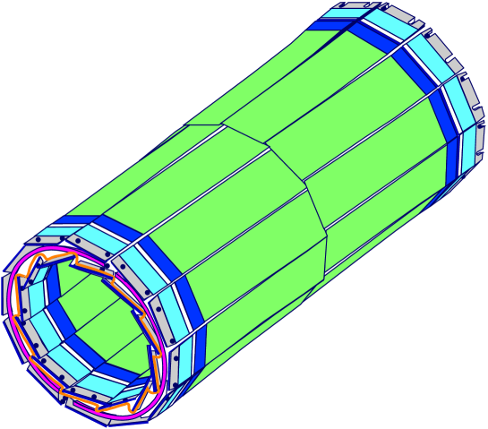
Figure 2.7: Perspective view of the SMD.

The principle of detection of the silicon microstrip (described in Fig. 2.8) is somewhat similar to that of the time expansion chamber, but, of course, the medium is different. The detection, here, benefits from the semi-conductor properties of the material. A particle passing through the silicon sensor will produce electron-hole pairs. By applying a voltage bias between the two sides of the sensor, holes and electrons will drift to the nearest strips on both surfaces, allowing a simultaneous measurement of the $r\phi$ and $rz$ coordinates.

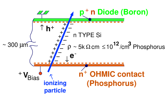
Figure 2.8: The principle of detection of the SMD.

2.3 Data processing

The way in which particles are detected and recorded by the various subdetectors can sometimes be very far from the physical quantities we want to measure. Therefore, it is necessary to translate the information coming from the detector into more convenient variables, which can later be used to perform physics analyses such as those described in this thesis.

The treatment of the data requires three main steps. The first one is, of course, to decide if the signals emitted by a detector are relevant to a physical process of interest. This role is attributed to the trigger systems.

The next step is the reconstruction of the data, which translates detector response into physical quantities and stores this information on storage media for later use.

The third step which is needed, even if it does not directly concern the data themselves, is very important, it is the detector simulation. It enables us to understand (and to reproduce) the response of the detector components to the passage of particles, from a given physics process. Therefore, it helps us to understand the data and how particles interact with the detector.

2.3.1 Trigger system

No matter how relevant the information coming from the detector, the complete readout sequence of an event takes about $500\mu\text{s}$ (corresponding to the time of 22 beam crossings), during which the detector cannot process any new events. Therefore, a multi-level trigger system is implemented to reduce this dead time by allowing abortion of the readout sequence as soon as possible if a piece of information is found to be faulty. This enables the detector to start sooner a new readout sequence, and hence the recording of a good event.

The goal of the trigger system is to improve the interface between the detector and the data acquisition system (DAQ). Furthermore, it decides what can be trusted as relevant for physics analysis and should be written onto tape, thus reducing both the amount of memory space and the time lost in recording useless information. From the $45\text{kHz}$ collision only a few Hz can be stored on tape. The trigger ensures a certain level of quality of the information written on tape.

The trigger system proceeds in a small number of steps: At first, it has to decide, from signals emitted by a detector component, if these signals are compatible with an interaction. Then, if the signal is relevant to an collision, it decides, depending on the quality of the response of the subdetectors, to allow or to veto the storage on tape of these signals as an event.

There are three levels of trigger. The difference between the three levels is the complexity of the operations treated and the time needed to perform these calculations. Such a configuration allows a lower-level trigger to abort the readout sequence before higher-level triggers have completed more time consuming operations, and hence allows to save time in the readout process.

Level-1

The first-level trigger is a fast-response trigger. It consists of 5 independent sub-triggers, the energy trigger (which analyses the response from the calorimeters), the TEC trigger, the muon trigger (dedicated to the response of the muon chambers), the scintillator trigger, and the beamgate triggers. The role of the first-level trigger is to initiate the readout sequence if an collision is detected and to perform simple tests on an event in order to decide to keep it or not for further processing. Its decision time is about $20\mu\text{s}$. In order to pass the level-1 trigger, the event has to be selected by at least 1 of the 5 sub-triggers.

Level-2

The level-2 trigger works in parallel to the first-level trigger and has access to the same information. It has more time to proceed to a decision, however. Only events which were selected by only one level-1 sub-trigger are considered by the level-2 trigger. Events which were selected by more than one level-1 sub-trigger are automatically selected. The level-2 trigger is aimed at rejecting the most obvious background events, such as cosmic events (a muon produced by cosmic rays), detector noise, and interaction of the beam with residual gas (beam-gas) or with the wall of the beam pipe (beam-wall).

Level-3

The level-3 trigger uses the full data information and is able to perform full reconstruction of the data. It also has more time to perform more complex calculations, correlating several level-1 sub-triggers relevant to a subdetector. A level-3 trigger is implemented for each subdetector. For example, events which are selected by the TEC trigger are required to have tracks correlated with energy deposits in the calorimeter. Finally, if an event is selected by a level-3 trigger, it is written onto tape. This takes $500\mu\text{s}$.

The accepted events are grouped into runs of about 5000 events, corresponding (originally) to the tape capacity but also to a constant state of activity of the detector, a new run being initialized in case of change of status of the detector.

For our analysis, the events are required to originate from runs where TEC, SMD, HCAL and ECAL triggers were active. This ensures a uniform level of quality for the full data sample, which decreases the systematic uncertainties.

2.3.2 Event reconstruction

The information written onto tape during the data acquisition consists essentially of the recording of the various signals emitted by the detector. This information cannot be used directly in physics analysis. Further processing is, therefore, needed in order to extract the physical quantities relevant to particle physics analysis.

The reconstruction proceeds in two steps. In the first step, using the program package REL3, the various signals coming from one subdetector are combined into a primitive object, characteristic of this subdetector. The second step, by means of the subprogram AXL3, processes these objects correlating the information from various subdetectors, to obtain a class of objects relevant to physics analysis. There are several objects related to the main detector components. The following describes briefly the objects used in the present analysis.

• ASRC’s (AXL3 Smallest Resolvable Clusters), or simply clusters: These objects are obtained by combining the information from the calorimeters (both hadronic and electromagnetic). They correspond to the smallest energy deposit which can be resolved. The ASRC’s are used in this analysis to select hadronic events (Sect. 3.1).

• ATRK’s (AXL3 TRacKs), also called tracks: These objects are obtained by combining TEC, SMD and Z chamber information. They are also required to be matched with a calorimeter object. The ATRK’s correspond to charged particles detected in the inner part of the L3 detector. They are the main objects used in this analysis.

2.3.3 Event simulation

Natural ways to understand the data include their comparison to theoretical expectation or to try to reproduce their signature using a Monte Carlo generator which incorporates the present knowledge we already have of a reaction. The generation of Monte Carlo events is thus very important for our understanding of the underlying physics.

However, it must be kept in mind, that the detector is not $100\%$ efficient and part of the information can be lost or distorted by the various materials used for the detection. It is mandatory to understand the interaction between particles and the detector material, as well as the effect induced by the various parts of the detector. This understanding is incorporated into a Monte Carlo program which simulates the perturbation induced by the detector and the detection itself.

Therefore, the events generated by the Monte Carlo event generator are also processed by SIL3 [37], a program based on the GEANT program (a general program package designed to simulate interactions between particles and detector materials) and aimed at simulating the whole chain of detection (from the detection itself to the DAQ) of the L3 detector.

There are two levels of simulation in the L3 collaboration. The first is called ideal simulation. It corresponds to the simulation of an “ideal” L3 detector for which all the various detector channels work at their maximum efficiency.

The second level of simulation is called realistic simulation. This simulation is time dependent and the major changes in the detector during a period of data taking are incorporated. This can be the permanent loss of detection channels, such as a dead crystal of BGO, noisy electronic channels, or eventual problems in a subdetector causing its inactivity. As for the TEC, the high voltage is permanently monitored ( a status is recorded every five minutes) during data taking in order to incorporate in the realistic simulation the loss of power (and consequently the partial or total loss of data) in one or all sectors. The same runs used for the data are used in the Monte Carlo simulation.

The analysis reported here uses realistic Monte Carlo simulation.

Chapter 3 Event selection

This analysis is based on data collected by the L3 detector in 1994 and 1995 at an energy equal to the mass of the $\mathrm{Z}^{0}$ boson. The data sample corresponds to approximately two million hadronic $\mathrm{Z}^{0}$ decays. Since the analysis makes extensive use of the reconstructed charged-particle multiplicity distribution, not only a good purity in hadronic events is needed, but also a well understood selection of the charged tracks. This understanding cannot be achieved without a precise simulation of the Central Tracker of L3.

In order to fulfill the requirements of purity and track selection, the events are selected in a two-step procedure. The first step selects hadronic events and removes most of the background, using the energy measured in the electro-magnetic and hadronic calorimeters. The second step of the selection, more specific to this analysis, is aimed at selecting good tracks measured with the Central Tracking Detector, in order to obtain the best reliability of data and Monte Carlo simulation while keeping the number of tracks in the event as large as possible. Good agreement between data and simulation is essential in order to reconstruct the charged-particle multiplicity distribution, since this reconstruction is strongly dependent on the description of the inefficiencies of the L3 detector, which are obtained from simulations.

Also used in our analysis are samples obtained from light- and b-quark events, separately. The procedure used to extract the charged-particle multiplicity distributions from these particular types of events is described in the third section.

3.1 Calorimeter based selection

The selection of hadronic events is based on the energy measured in the hadronic and electro-magnetic calorimeters. Its main purpose is to remove as large as possible a fraction of the background in such a way that this does not affect the measurement of the charged tracks in TEC. Of course, the background could be eliminated using the Tracking Chamber only. However, the cost to pay in terms of efficiency would be rather large, since this would prevent any measurement of the low-multiplicity events, which are highly contaminated by many background sources (described later).

The background sources can be divided into two main categories [38]: The first category consists of events originating from leptonic $\mathrm{Z}^{0}$ channels (, $\mu^{+}\mu^{-}$, $\tau^{+}\tau^{-}$). The second category, called non-resonant background, contains sources such as two-photon interactions, as well as beam-wall and beam-gas events.

A preliminary cut on the calorimeter cluster energy removes calorimeter clusters with an energy deposit smaller than $100\MeV$, which are highly contaminated by electronic noise. Once these clusters are removed, we can proceed to the event selection. For that, we need to define a set of useful variables. First of all we define the visible energy, $E^{\mathrm{cal}}_{\mathrm{vis}}$ of an event as the sum of all (remaining) cluster energies $E^{\text{cal}}_{i}$. In a similar manner we define the vectorial energy sum $\vec{E}^{\text{cal}}$, obtained by summing the cluster energy along the particle direction as seen from the interaction point, $\vec{n}_{i}$:

$$E^{\mathrm{cal}}_{\mathrm{vis}}={\underset{i}{\sum}}E^{\mathrm{cal}}_{i}\phantom{2}\text{ and }\phantom{2}\vec{E}^{\text{cal}}={\underset{i}{\sum}}E^{\mathrm{cal}}_{i}\cdot\vec{n}_{i}.$$ (3.1)

We also define the longitudinal and the transverse energy imbalance, $E^{\mathrm{cal}}_{\sslash}\text{ and }E^{\mathrm{cal}}_{\perp}$ as the projection along the $z$ axis and in the plane perpendicular to the $z$ axis of $\vec{E}^{\text{cal}}$ normalized to the visible energy $E^{\mathrm{cal}}_{\mathrm{vis}}$, respectively:

$$E^{\mathrm{cal}}_{\sslash}=\frac{|E^{\mathrm{cal}}_{z}|}{E^{\mathrm{cal}}_{\mathrm{vis}}}\phantom{2}\text{ and }\phantom{2}E^{\mathrm{cal}}_{\perp}=\frac{\sqrt{(E^{\mathrm{cal}}_{x})^{2}+(E^{\mathrm{cal}}_{y})^{2}}}{E^{\mathrm{cal}}_{\mathrm{vis}}}.$$ (3.2)

Cuts on the rescaled visible energy

Hadronic $\mathrm{Z}^{0}$ events are characterized by a visible energy centered around the center of mass energy, $\sqrt{s}$. Non-resonant background, in particular beam-wall, beam-gas and two-photon events, which typically have a much lower visible energy, are easily discarded by a cut on $E^{\mathrm{cal}}_{\mathrm{vis}}{}$ (Fig. 3.1). Selected events are required to satisfy

$$0.5<\frac{E^{\mathrm{cal}}_{\mathrm{vis}}}{\sqrt{s}}<1.5.$$ (3.3)

The role of the upper cut is to remove Bhabha events which are located at scaled energy higher than 1.5 because of the scaling factors (G-factors), which are used to take into account a shift to lower value of the energy detected for hadrons. Since the energy of electrons is fully detected, they should not be subjected to this shift consequently end up with an higher scaled energy.

Figure 3.1: Distribution of the visible energy rescaled to $\sqrt{s}$ for the data (dots) compared to events simulated with JETSET 7.4 PS (line). As for all the following selection plots, all cuts are applied, except that on the variable plotted, the latter cut being represented by arrows.

Cut on the number of ASRC clusters

Hadronic events usually have a larger particle multiplicity than other processes. Hence, a way to reduce the background contamination is to cut on low-multiplicity events. By requiring that events have at least 14 ASRC clusters, most of the , $\mu^{+}\mu^{-}$ and $\tau^{+}\tau^{-}$ background is eliminated (Fig. 3.2). It must be noted that the large discrepancy between Monte-Carlo and data for large multiplicities is due to an incorrect description of hadronic showers in the BGO crystals of the ECAL and not to some kind of background contamination. Therefore, there is no reason in this analysis, which uses only charged tracks, to cut on large cluster multiplicities.

Figure 3.2: Distribution of the number of ASRC clusters for the data (dots) compared to JETSET 7.4 PS (line) predictions.

Cuts on the energy imbalance

Since at LEP, the laboratory frame for collisions coincides with the center of mass frame, hadronic events are well balanced in energy flow. This is not the case for the non-resonant background, which usually has a large longitudinal energy imbalance. Furthermore, due to $\tau$ decay into a quark or a lepton via the emission of neutrinos, the $\tau^{+}\tau^{-}$ background has a larger energy imbalance than the other  channels. As shown in Fig. 3.3, we require the longitudinal energy imbalance $E^{\mathrm{cal}}_{\sslash}$ to be smaller than 0.4 and the transverse energy imbalance $E^{\mathrm{cal}}_{\perp}$ to be smaller than 0.6.

Figure 3.3: Transverse and longitudinal energy imbalance for the data (dots) and for the Monte-Carlo (line).

Cut on the direction of the thrust axis

To ensure that the event lies within the full acceptance of the TEC and since the TEC only poorly covers the end-cap region of the detector, we use only events which have the direction of the thrust axis within the barrel of the detector. Barrel events are selected by requiring $|\cos(\theta^{\mathrm{cal}}_{\mathrm{th}})|<0.74$ (Fig. 3.4), where $\theta^{\mathrm{cal}}_{\mathrm{th}}$ is the polar angle of the event thrust axis determined from calorimeter clusters.

Figure 3.4: Distribution of $\cos(\theta^{\mathrm{cal}}_{\mathrm{th}})$ for the data (dots) and for the Monte-Carlo (line).

To summarize, the calorimeter selection criteria of hadronic events are:

• $0.5<E^{\mathrm{cal}}_{\mathrm{vis}}/\sqrt{(}s)<1.5$

• $N_{\mathrm{clus}}>14$

• $E^{\mathrm{cal}}_{\sslash}<0.4\text{ and }E^{\mathrm{cal}}_{\perp}<0.6$

• $|\cos(\theta^{\mathrm{cal}}_{\mathrm{th}})|<0.74.$

After having applied these cuts, approximately one million hadronic events remain, with a purity around $98\%$ [38]. All the non-hadronic background ( background which does not decay hadronically) has been removed, with the exception of $1.3\%$ of the $\tau^{+}\tau^{-}$ background, $0.23\%$ of the $\ee\text{q}\bar{\text{q}}$ background and $1.1\%$ of the $\tau^{+}\tau^{-}$ background. This calorimeter pre-selection has the advantage of eliminating the background while being largely decoupled from the track selection, allowing relatively weak cuts on track momenta. The next step is the selection of charged particles using the central tracking detector.

3.2 TEC based selection

The main goals of the TEC track selection are

1. to remove badly reconstructed tracks and

2. to improve the simulation of track inefficiencies,

in order to have the best possible reliability of the central tracking detector simulation, on which the reconstruction of the charged-particle multiplicity and momentum distributions strongly depends.

Since the event selection by means of the calorimeter clusters has rejected most of the background, only a few cuts will be applied on an event basis.

3.2.1 Track quality criteria

Transverse momentum

The transverse momentum of a track is calculated from its curvature imposed by the magnetic field in the plane perpendicular to the beam axis. Tracks having a low transverse momentum are easily contaminated by noise and must be removed. Hence, the transverse momentum is required to be larger than $150\MeV/c$ (Fig. 3.5)

Figure 3.5: Distribution of track transverse momenta for the data (dots) and for the Monte-Carlo (line).

Number of hits

When a particle, originating from the interaction point and flying across the TEC, passes near a wire of TEC, it causes a local ionization of the gas leading to an electric discharge on the wire. This is called a hit. There are 62 wires in the TEC, 8 wires in the inner TEC and 54 in the outer TEC. The larger the number of hits, the better is the resolution of the transverse momentum, since the curvature is calculated from the path formed by the subsequent hits.

Misreconstructed track segments usually have a small number of hits. Furthermore, the absence of a hit in the inner TEC increases strongly the chance of misreconstruction of a track, since the track is not measured close to the interaction region. Therefore, we require at least one hit in the inner TEC, which ensures that tracks come from the interaction region (Fig. 3.6). It will also help to solve the left-right ambiguity which occurs when detecting charged particle with a wire chamber. As the hits recorded from a charged particle passing near an anode wire do not tell on which side of the wire, the charged particle has been detected, two tracks can be reconstructed from a same set of hits. One track corresponding to the real track of the charged particle, the other, the mirror track, symmetric with respect to the wire of the track of the charged particle.

Since the agreement between the data and the Monte Carlo simulation is rather poor for the distribution of the number of TEC hits (Fig. 3.7 (a)), the cut is chosen to lie in the middle of a region of the distribution where the variation of the disagreement between data and Monte Carlo is stable and no big change from bin to bin in this disagreement is expected. Therefore, the number of hits in the TEC is required to be at least 25. Loss in track momentum resolution, which could result from the use of such a low minimum requirement on the number of hits, is minimized by the previous requirement of at least one hit in the inner TEC and also by the choice of a rather large span (see below).

Figure 3.6: Distribution of the number of hits in the inner TEC for the data (dots) and for the Monte Carlo (lines).

Span of a track

Tracks are reconstructed by combining hits. Sometimes, hits from different tracks are mistakenly combined. Since these tracks usually have a smaller length than well reconstructed tracks, it is possible to remove most of these tracks by requiring a minimum length for each track. The length of a track is given by the span defined as:

$\mathrm{Span}=\mathrm{W}_{\mathrm{first}}-\mathrm{W}_{\mathrm{last}}+1,$

where $\mathrm{W}_{\mathrm{first}}$ and $\mathrm{W}_{\mathrm{last}}$ are the wire numbers of the innermost hit ( the wire on which the first hit is left by the particle coming from the interaction point when entering the TEC) and of the outermost hit ( the wire on which the last hit has been recorded before the particle leaves the TEC) recorded for a track. All tracks are required to have a span of at least 40 (Fig. 3.7 (b)).

Figure 3.7: Distribution of the number of hits in the whole TEC (left plot) and of the span of tracks (right plot) for the data (dots) and for the Monte-Carlo (line).

Distance of closest approach

To check if a track originates from the interaction vertex, each track is extrapolated back to the interaction vertex. The distance of closest approach (DCA) to the interaction vertex is then calculated in the plane transverse to the beam direction. In order to ensure that a track is coming from the interaction vertex, a DCA smaller than 10mm is required (Fig. 3.8).

Figure 3.8: Distance of closest approach of tracks for the data (dots) and for the Monte-Carlo (line).

Azimuthal track angle $\phi$

Due to a wrong simulation of inefficiencies of two TEC sectors, large discrepancies between data and Monte Carlo are seen in the azimuthal angular distribution for the two half-sectors located at $45^{\circ}<\phi<52.5^{\circ}$ and $225^{\circ}<\phi<232.5^{\circ}$ (Fig. 3.9). Therefore, tracks located in these two half sectors were simply removed from the analysis.

Figure 3.9: Distribution of the azimuthal $\phi$ track angle for the data (dots) and for the Monte-Carlo (line).

3.2.2 TEC inefficiencies

During data taking, from time to time, high background levels, which are likely to generate overcurrents or trips of anodes and cathodes, can cause the TEC to be partly or totally turned off. This leads to a temporary loss of efficiency in certain TEC sectors or in the whole TEC.

The Monte Carlo simulation takes into account the major part of such problems occurring during a data taking period (rdvn format), but not if the problem has only occurred during a short period of time.

Finally, it appears that the Monte Carlo simulation underestimates the track losses close to the anodes and cathodes of the TEC. This discrepancy is clearly seen in the distribution of outer $\phi$ local, , the distribution of the angle, $\phi_{\text{loc}}$, between the track and the closest outer TEC anode (Fig. 3.10).

In order to improve the TEC inefficiency simulation, a random rejection of Monte Carlo tracks is applied two degrees around anodes and cathodes. The random rejection leads to a better matching for the azimuthal angular distribution between data and simulation and, therefore, to an overall better agreement between data and Monte Carlo.

Figure 3.10: Distribution of the $\phi$ local angle of tracks for the data (dots) and for the initial Monte Carlo (solid line) and for the Monte Carlo with random rejection (dashed line).

3.2.3 Event selection

Even though we have already applied a hadronic event selection using calorimeter clusters, a few additional cuts are needed. In order to reject the remaining $\tau^{+}\tau^{-}$ background, we impose a cut on the second largest angle $\phi_{2}$ between any two neighboring tracks in the $r\phi$ plane. Selected events are required to have their $\phi_{2}$ angle between $20^{\circ}$ and $170^{\circ}$ (Fig. 3.11(a)) which optimizes the rejection of $\tau^{+}\tau^{-}$ background without rejecting too large a fraction of the hadronic $\mathrm{Z}^{0}$ events.

Furthermore, events are required to have their thrust axis in the barrel of the TEC. For that purpose, $|\cos(\theta^{\mathrm{TEC}}_{\mathrm{th}})|$ is required to be less than 0.7, where $\theta^{\mathrm{TEC}}_{\mathrm{th}}$ is the polar angle of the event thrust axis determined from charged tracks (Fig. 3.11(b)). After selection, the purity in hadronic $\mathrm{Z}^{0}$ events is about $99\%$. What remains in the selected sample is $0.19\%$ of the $\tau^{+}\tau^{-}$background and $0.07\%$ of both the $\tau^{+}\tau^{-}$and the $\ee\text{q}\bar{\text{q}}$ background.

About 1 million events survive the selection.

Figure 3.11: Distribution of $\phi_{2}$ (a) and of $|\cos(\theta^{\mathrm{TEC}}_{\mathrm{th}})|$ (b) for the data (dots) and for the Monte Carlo (line). The shaded area in (a) indicates $\tau^{+}\tau^{-}$ background generated with the KORALZ Monte Carlo and is normalized to the relative production rate.

3.3 Light- and b-quark event selection

The selection of light-quark events ($\text{Z}\rightarrow$$\text{}\text{u}\bar{\text{u}}\text{, }\text{d}\bar{\text{d}}\text{, }\text{s}\bar{\text{s}}\text{ or }\text{c}\bar{\text{c}}$) and of b-quark events ($\Zbb$) proceeds in two steps. In the first step, a b-tag algorithm is used to define high purity samples of light- and b-quark events. The second step applies the above-described general hadronic event selection procedures in order to obtain samples from which charged-particle multiplicity distributions can be extracted.

The b-tag algorithm which is applied to discriminate between light-quark and b-quark events, relies on the full three-dimensional information on tracks recorded in the central tracking detector (TEC and SMD), in order to compute the probability that a track comes from the primary vertex. The method is fully described in [39], but the main steps of the method are briefly summarized here.

The algorithm starts with the three-dimensional reconstruction of the primary vertex by minimizing

$$\chi^{2}_{N_{\text{trk}}}=\overset{N_{\text{trk}}}{\underset{i=1}{\sum}}(\vec{t}_{i}-\vec{f}(\vec{\nu},\vec{q}_{i}))^{T}G^{-1}_{i}(\vec{t}_{i}-\vec{f}(\vec{\nu},\vec{q}_{i}))+(\vec{\nu}-\vec{\nu}_{\text{fill}})^{T}V^{-1}_{\text{fill}}(\vec{\nu}-\vec{\nu}_{\text{fill}}),$$ (3.4)

where $N_{\text{trk}}$ is the number of tracks, $\vec{t}_{i}$ is the vector of measured parameters for the $i^{\text{th}}$ track, $G_{i}$ is the corresponding covariance matrix, $\vec{f}(\vec{\nu},\vec{q}_{i})$ is the corresponding prediction assuming that the track originates at the vertex $\vec{\nu}$ with momentum $\vec{q}_{i}$, $\vec{\nu}_{\text{fill}}$ is the so-called fill vertex, a measure of the position of the beam spot, and $V_{\text{fill}}$ is its covariance matrix. The $N_{\text{trk}}$ tracks involved in the $\chi^{2}$ have to satisfy the following criteria:

• being fitted with the Kalman filter [40],

• $|d_{r\phi}|<\text{min}(10\text{mm},5\sigma(d_{r\phi}))$, where $d_{r\phi}$ and $\sigma(d_{r\phi})$ are the distance of closest approach in the $xy$ plane and its error,

• $|d_{sz}|<100\text{mm}$, $d_{sz}$ being the distance of closest approach in the $sz$ plane.

If $P(\chi^{2}_{N_{\text{trk}}})$ is less than $4\%$ for a particular event, tracks are removed one by one and the $\chi^{2}$ is redetermined after having removed each track in turn. This results in the probability $P_{i}=P(\chi^{2}_{N_{\text{trk}}}-\chi^{2}_{N_{\text{trk}}-1,i})$ for the case that track $i$ is removed. Tracks, for which $P_{i}$ and $P(\chi^{2}_{N_{\text{trk}}})$ are both less than $2\%$ are definitely removed. The fit procedure is repeated until no further track needs to be removed. Primary vertices having less than three remaining tracks are rejected.

Once the primary vertex has been reconstructed, the decay lengths $L_{r\phi}$ and $L_{sz}$ measured in the $r\phi$ and $sz$ planes, respectively, can be estimated. They are defined as the distance in the $r\phi$ and $sz$ (see Fig. 3.12) planes between the impact point of a track and the primary vertex and correspond to independent measurements of the true decay length of the B hadron. They are used to compute an average decay length $L$.

From the significance defined as $S=L/\sigma_{L}$, the probability, $P(S_{i})$, that a track with decay length, $L$, originates from the primary vertex, is computed. The track probabilities $P(S_{j})$ are combined into an event probability, $P_{\text{event}}$, which carries the sensitivity for an event to be a b-quark event,

$$P_{\text{event}}=\frac{\Pi}{2^{N}}\overset{N-1}{\underset{i=0}{\sum}}\overset{N}{\underset{j=i+1}{\sum}}C^{N}_{j}\frac{(-\ln\Pi)^{i}}{i!}\text{, where }\Pi=\overset{N_{+}}{\underset{j=1}{\prod}}P(S_{j}),$$ (3.5)

where $N_{+}$ is the number of tracks which have a positively signed decay length [39].

Due to the long life time and, hence, the long decay length of b hadrons, the probability $P_{\text{event}}$ is close to zero for a b-quark event, while for other types of events, $P_{\text{event}}$, is larger. Therefore, to emphasize the low probability region, a discriminant $\delta$ is defined as

$$\delta=-\log P_{\text{event}}.$$ (3.6)

The distribution of this discriminant is shown in Fig. 3.14 for the 1994 (left) and the 1995 (right) data taking periods, for both the data and JETSET for all events, together with the separate JETSET discriminant distributions for light-quark events and for b-quark events. The selection or the rejection of b-quark events is based on the discriminant $\delta$. Light-quark events are selected by $\delta<\delta_{\text{cut}}$, and b-quark events by $\delta>\delta_{\text{cut}}$. The purity and efficiency of the light-quark sample are shown in Fig. 3.14 as a function of $\delta_{\text{cut}}$ for the 1994 data sample (top left) and for the 1995 data sample (top right). The purity and efficiency of the b-quark sample are shown in Fig. 3.14 as a function of $\delta_{\text{cut}}$ for the 1994 data sample (bottom left) and for the 1995 data sample (bottom right).

To minimize the size of the corrections which will have to be applied to the tagged samples in order to get pure light- and b-quark samples, high purities in light and b quarks are required. Therefore, the tagged light-quark event sample is selected by requiring a discriminant value $\delta<1.2$. For this cut, the purity and efficiency of the sample in light quarks for 1994 are $93.4\%$ and $89.2\%$, respectively, for 1995, $93.0\%$ and $91.6\%$. The tagged b-quark event sample is selected by requiring a discriminant value $\delta>3.4$, which leads to a purity and efficiency in b-quarks for 1994 of $95.2\%$ and $38.9\%$, respectively, and for 1995 of $97.0\%$ and $37.1\%$. These purities and efficiencies are not altered by the event selection.

Once the light- and b-quark samples are selected, we apply to them the same selection criteria which are applied to the full sample, as described previously in Sects. 3.1 and 3.2.1.

Figure 3.12: Distance of closest approach of a track, $d_{sz}$, together with its decay length, $L_{sz}$ in the $sz$ plane.

Figure 3.13: Event discriminant distribution for the 1994 data (left) and for the 1995 data (right) compared with the discriminant distributions of the Monte Carlo for all events, b-quark events and light-quark events.

Figure 3.14: The efficiency and purity in the light-quark sample for the year 1994 (a) and 1995 (b) obtained by varying the cut on the discriminant value aimed to select light quarks ($\delta<\delta_{\text{cut}}$), and the efficiency and purity in the b-quark sample (right) obtained by varying the cut on the discriminant value aimed to select b quarks ($\delta>\delta_{\text{cut}}$) for the year 1994 (c) and for 1995 (d).

Chapter 4 The charged-particle multiplicity distribution

Besides its theoretical interest discussed in Sect. 1.4, the interest in the charged-particle multiplicity distribution arises from the fact that the detection of charged particles is far more easy than the detection of neutral particles. To measure the full multiplicity distribution (charged and neutral particles), we would have to rely on the detection of energy deposits in the calorimeter, the calorimeter clusters. Since these clusters can represent from a fraction of the energy up to the whole energy of a particle, the correspondence between clusters and particles is rather difficult to establish. Therefore, the extrapolation from energy clusters to particles would depend a lot on the simulation. As we have seen in the previous chapter, due to an underestimation of the noise in the calorimeter, the agreement in terms of clusters between data and simulation is not good enough to perform such a measurement.

A charged particle is detected as a track in the Central Tracking Chamber. Unlike a calorimeter cluster, a track and its kinematical content represents a particle and not a fragment of a particle (the track quality selections eliminate most of the badly measured or split tracks). This increases both the reliability and the traceability of the final result since we can keep track of the charged particles from their detection to their reconstruction. However, an accurate treatment is still needed to reconstruct the charged-particle multiplicity distribution.

In the first section of this chapter, we discuss the steps needed to reconstruct the charged-particle multiplicity distribution for the full, light- and b-quark samples, starting from the measured raw-data charged-particle multiplicity distribution. The next two sections introduce the calculation used to estimate their statistical errors and their systematic uncertainties. The resulting charged-particle multiplicity distributions and their principal moments are presented and discussed in the final section of this chapter.

4.1 Reconstruction of the multiplicity distribution

Because of the limited acceptance of the detector and of the selection procedures which were used to obtain a pure sample of hadronic decays, not only do events escape both the detection and selection processes, but also do the detected events usually contain fewer particles than were produced. The most dramatic example of this effect is given in Fig. 4.1 by the charged-particle multiplicity distribution itself. If all charged particles in an event were detected, charge conservation implies that their number would always be even. However, as shown here, we find both even and odd multiplicities. Therefore, the treatment needed to reconstruct the charged-particle multiplicity has to take into account not only the undetected events, but also the undetected particles within an event. We therefore proceed in two steps. The first step uses an unfolding method which corrects the number of particles in an event. The second step corrects for event selection, including light- or b-quark selection and initial-state radiation. An additional correction is applied to take into account the charged $\text{K}^{0}_{\text{s}}\text{ and }\Lambda$ decay products.

As a convention, and unless otherwise stated, we refer by $N(n)$ to the distribution of the number of events with a particle multiplicity $n$, and by $P(n)$ to the distribution of our estimate of the probability to obtain an event with a particle multiplicity of $n$,

$$P(n)=\frac{N(n)}{\underset{i}{\sum}N(i)}.$$ (4.1)

The same convention will also apply to matrices.

Figure 4.1: The detected charged-particle multiplicity distribution of the 1994 data.

Correction for inefficiencies and limited acceptance of the detector

The most common way to correct for detector inefficiencies consists of multiplying bin-by-bin the raw data distribution of a given variable, $V^{\text{data}}_{\text{raw}}$, by a correction factor which is the ratio of the distribution of the variable, $V^{\text{MC}}_{\text{prod}}$, generated by Monte Carlo in the case of a detector working at $100\%$ efficiency and the distribution of the variable, $V^{\text{MC}}_{\text{det}}$, generated by Monte Carlo, passed through the simulation of the detector, reconstructed and selected as the data,

$$V^{\text{data}}_{\text{cor}}=V^{\text{data}}_{\text{raw}}\frac{V^{\text{MC}}_{\text{prod}}}{V^{\text{MC}}_{\text{det}}}.$$ (4.2)

However, this type of correction can only be used when the simulated and generated distributions are consistent with each other. ( have the same number of bins). Because the method intrinsically assumes the independence of each bin, it is better suited to correct for a global effect such as, , a loss of events due to the selection procedure. Although this method will be used for that purpose later, it is inappropriate here because of bin-to-bin migration. This is not necessarily localized to adjacent bins and, therefore, cannot be treated by simply changing the width of the bins in such way that the bin-to-bin migration would be taken into account. Due to the imperfection of the detection process (not only the detector itself, but also the track reconstruction and track quality cuts), the detected multiplicity is very often different from the original multiplicity. One can have detected multiplicities smaller or larger than the ones produced (as shown in Fig. 4.2). Furthermore, this effect of the bin-to-bin migration depends only in a non-trivial way to the number of particle produced and cannot be corrected without a full simulation of the detector. Therefore, another method is needed to take into account, as properly as possible, the bin migrations between produced and detected multiplicities. This is done by a so-called unfolding method.

The unfolding method makes use of the detector response matrix, $\mathcal{N}$, which takes the bin migrations into account. For each Monte Carlo event, this matrix $\mathcal{N}$ keeps track of the number of produced charged particles, $n$, and its associated number of detected tracks, $n_{\text{det}}$, which have been processed and selected in the same way as the data tracks. Each matrix element $\mathcal{N}(n_{\mathrm{det}},n)$ of $\mathcal{N}$ corresponds to the number of Monte Carlo events which have $n$ produced charged particles and $n_{\text{det}}$ detected tracks. The matrix found using events generated with JETSET is shown in Fig. 4.2. The probability of detecting $n_{\text{det}}$ tracks, $P(n_{\text{det}})$, is related to the probability distribution of produced charged particles, $P(n)$ by

$$P(n_{\text{det}})={\underset{n}{\sum}}\frac{\mathcal{N}(n_{\mathrm{det}},n)}{{\underset{n_{\mathrm{det}}}{\sum}}\mathcal{N}(n_{\mathrm{det}},n)}P(n),$$ (4.3)

Defining the migration matrix $\mathcal{M}$ by

$$\mathcal{M}(n_{\text{det}},n)=\frac{\mathcal{N}(n_{\mathrm{det}},n)}{{\underset{n_{\mathrm{det}}}{\sum}}\mathcal{N}(n_{\mathrm{det}},n)}.$$ (4.4)

Eq. (4.3) can be rewritten as

$$P_{\text{det}}=\mathcal{M}P_{\text{prod}},$$ (4.5)

where $P_{\text{det}}$ and $P_{\text{prod}}$ are vectors whose elements are $P(n_{\text{det}})$ and $P(n)$, respectively.

To estimate the produced multiplicity distribution of the data, $P^{\text{data}}_{\text{prod}}$, we can invert Eq. (4.5),

$$P^{\text{data}}_{\text{prod}}=\mathcal{I}P^{\text{raw}}_{\text{det}},$$ (4.6)

where $\mathcal{I}$ is obtained in a same manner as $\mathcal{M}$

$$\mathcal{I}(n,n_{\text{det}})=\frac{\mathcal{N}^{\text{T}}(n,n_{\mathrm{det}})}{{\underset{n}{\sum}}\mathcal{N}^{\text{T}}(n,n_{\mathrm{det}})}.$$ (4.7)

Note that $\mathcal{I}\neq\mathcal{M}^{\text{T}}$ because of different normalizations. The normalization of Eq. (4.4) makes $\mathcal{M}$ independent of the multiplicity distribution of the event generator. But this is not the case for Eq. (4.7). Consequently, the use of the matrix $\mathcal{I}$ in Eq. (4.6) could bias the result towards the distribution of the event generator.

Figure 4.2: The response matrix of the detector obtained with JETSET Monte Carlo.

Therefore, we use a more elaborate method, known as Bayesian unfolding, in which Eq. (4.5) is used iteratively [41],[42]. The probabilities of producing $n$ particles and of detecting $n_{\text{det}}$ tracks are related by Bayes’ theorem:

$$\mathcal{M}(n_{\text{det}},n)P(n)=\mathcal{I}(n,n_{\text{det}})P(n_{\text{det}}).$$ (4.8)

Hence

$$\mathcal{I}(n,n_{\text{det}})=\mathcal{M}(n_{\text{det}},n)\frac{P(n)}{P(n_{\text{det}})}.$$ (4.9)

Taking $P(n_{\text{det}})$ from Equation (4.3), this becomes

$$\mathcal{I}(n,n_{\text{det}})=\frac{\mathcal{M}(n_{\text{det}},n)P(n)}{{\underset{n}{\sum}}\mathcal{M}(n_{\mathrm{det}},n)P(n)}.$$ (4.10)

Inserting this in Eq. (4.6) gives an estimate of the produced multiplicity distribution:

$$P^{\text{data}}(n)={\underset{n_{\mathrm{det}}}{\sum}}\frac{\mathcal{M}(n_{\text{det}},n)P(n)}{{\underset{n}{\sum}}\mathcal{M}(n_{\mathrm{det}},n)P(n)}P^{\text{raw}}(n_{\text{det}}).$$ (4.11)

This equation is the basis for the Bayesian unfolding. But instead of using directly the result of this equation, and in order to remove the bias due to the use of a limited statistics sample for the construction of the matrix $\mathcal{M}$, we will use Eq. (4.11) iteratively.

We start the iterative unfolding procedure by comparing the detected charged-particle multiplicity distribution of the data, $P^{\text{raw}}(n_{\text{det}})$ to $\sum\mathcal{M}(n_{\mathrm{det}},n)P^{(0)}(n)$, which, according to Eq. (4.3), corresponds to the detected distribution $P^{(0)}(n_{\text{det}})$. In principle, the initially produced distribution, $P^{(0)}(n)$, can be anything, but here we use the charged-particle multiplicity distribution produced from JETSET Monte Carlo, since we found that its fully simulated multiplicity distribution agrees rather well with the raw data. The $\chi^{2}/\text{dof}$ between the detected distributions, $P^{\text{raw}}(n_{\text{det}})$ and $P^{(0)}(n_{\text{det}})$ is calculated, and if it is larger than 1, the ratio $C^{(1)}(n_{\mathrm{det}})$ is calculated,

$$C^{(1)}(n_{\mathrm{det}})=\frac{P^{\mathrm{raw}}(n_{\mathrm{det}})}{{\underset{n}{\sum}}\mathcal{M}(n_{\mathrm{det}},n)P^{(0)}(n)}.$$ (4.12)

Using $C^{(1)}$ in Eq. (4.11), we can write

$$C^{(1)}(n)={\underset{n_{\mathrm{det}}}{\sum}}\mathcal{M}(n_{\mathrm{det}},n)C^{(1)}(n_{\mathrm{det}}),$$ (4.13)

with

$$C^{(1)}(n)=\frac{P^{(1)}(n)}{P^{(0)}(n)},$$ (4.14)

where $P^{(1)}(n)$ is the first-iteration estimate of the produced charged-particle multiplicity distribution of the data.

Using now $P^{(1)}(n)$ in Eq. (4.3), we can compare the detected charged-particle multiplicity distribution of the data $P^{\text{raw}}(n_{\text{det}})$ to the estimate of the detected charged-particle multiplicity distribution $P^{1}(n_{\mathrm{det}})$ at detected level,

$$P^{\text{(1)}}(n_{\text{det}})={\underset{n}{\sum}}\mathcal{M}(n_{\mathrm{det}},n)P^{\text{(1)}}(n).$$ (4.15)

Depending on the value of the $\chi^{2}$ between $P^{\text{raw}}(n_{\text{det}})$ and $P^{\text{(1)}}(n_{\text{det}})$, we proceed to the next iteration by repeating with $P^{(1)}(n)$ instead of $P^{(0)}(n)$ the whole procedure described in Eqs. (4.12) and (4.14), leading finally to the estimate of the charged-particle multiplicity distribution of the data for the second iteration,

$$P^{(2)}(n)=P^{\mathrm{(1)}}(n)C^{(2)}(n).$$ (4.16)

By generalizing this result to the $q^{\text{th}}$ iteration we have:

$$P^{(q)}(n)=P^{(q-1)}(n)C^{(q)}(n)=P^{(0)}(n)\overset{q}{\underset{i=1}{\prod}}C^{(i)}(n),$$ (4.17)

$$\text{where }C^{(i)}(n)={\underset{n_{\text{det}}}{\sum}}\mathcal{M}(n_{\text{det}},n)\frac{P^{\text{raw}}(n_{\text{det}})}{{\underset{n}{\sum}}\mathcal{M}(n_{\text{det}},n)P^{(i-1)}(n)}.$$ (4.18)

The iterative process is stopped when the $\chi^{2}/\text{dof}$ has become sufficiently small, , smaller than 1. This occurs after the second iteration. Therefore, $P^{(2)}(n)$ is taken as our estimate of the reconstructed charged-particle multiplicity distribution of the data,

$$P^{\text{rec}}(n)=P^{(2)}(n).$$ (4.19)

The unfolding method corrects only for detector inefficiencies, changing the multiplicity within a given event. In particular, it does not correct for events which were rejected by the event selection procedure. To obtain a fully corrected charged-particle multiplicity distribution, we, therefore, need additional factors.

Correction for event selection

We first correct for events which were removed by the event selection. This is done by applying correction factors (Fig. 4.3 (a)), which are obtained by taking the ratio of the charged-particle multiplicity distribution of all Monte Carlo events at generator level, $P^{\text{all}}_{\text{prod}}(n)$, to that of the generator level which, when fully simulated, pass the selection procedure, $P^{\text{acc}}_{\text{prod}}(n)$,

$$C_{\text{acc}}(n)=\frac{P^{\text{all}}_{\text{prod}}(n)}{P^{\text{acc}}_{\text{prod}}(n)}.$$ (4.20)

Figure 4.3: ratios $C_{\text{acc}}(n)$, (a), and $C_{\text{ISR}}(n)$, (b), to correct for event selection and for ISR, respectively.

Correction for Initial-State Radiation

Since we are interested in a pure sample of hadronic events at the $\mathrm{Z}^{0}$ energy, we also need to correct for Initial-State Radiation (ISR). This ISR refers to the emission of one or more photons by the electron or the positron, which shifts the energy of the event to a lower value. The ISR events have a signature similar to that of normal hadronic events, except that they have lower center of mass energies and, hence, lower charged-particle multiplicities. At the $\mathrm{Z}^{0}$ energy, these events represent only a small fraction of the hadronic events and are well simulated by Monte Carlo. Therefore, their contribution may be easily corrected by a simple correction factor, (Fig. 4.3 (b)), corresponding to the ratio of the charged-particle multiplicity distributions of Monte Carlo events generated with, $P^{\text{ISR}}(n)$, and without, $P^{\text{noISR}}(n)$, initial state radiation,

$$C_{\text{ISR}}(n)=\frac{P^{\text{noISR}}(n)}{P^{\text{ISR}}(n)}.$$ (4.21)

These two corrections are applied to the reconstructed charged-particle multiplicity distribution of the data, $P(n)$, to obtain finally a fully corrected charged-particle multiplicity distribution,

$$P(n)=C_{\text{acc}}(n)C_{\text{ISR}}(n)P^{\text{rec}}(n).$$ (4.22)

Correction for $\mathrm{K}^{0}_{\mathrm{s}}\text{ and }\Lambda$ decay products

In the context of the strong interaction, particles which decay weakly or electromagnetically are considered stable. However, experimentally it is more appropriate to consider particles which are detected. This leads to a problem in the case of $\mathrm{K}^{0}_{\mathrm{s}}$ and $\Lambda$, both of which can decay weakly to two charged particles which can be detected in L3. Therefore, the detected charged-particle multiplicity distribution contains charged particles produced in these decays. However, to obtain a charged-particle multiplicity distribution relevant to QCD, $\mathrm{K}^{0}_{\mathrm{s}}$ and $\Lambda$ should be considered stable. The necessary correction introduces the uncertainties on $\mathrm{K}^{0}_{\mathrm{s}}$ and $\Lambda$ production into the charged-particle multiplicity distribution. Particularly in the early days of LEP, these uncertainties were large, which led experiments to refrain from applying these corrections. At present, these uncertainties are much smaller. In the unfolding procedure, we have, therefore, corrected the data to obtain the multiplicity distribution that does not include $\mathrm{K}^{0}_{\mathrm{s}}$ and $\Lambda$ decay products. However, for comparison with other experiments, we also present the multiplicity distribution containing these decay products.

Inclusion of the $\mathrm{K}^{0}_{\mathrm{s}}$ and $\Lambda$ decay products corresponds to an increase of the number of charged particles in an event. The problem we are facing is then similar to the track migration problem caused by detector acceptance and inefficiencies. Therefore, $\mathrm{K}^{0}_{\mathrm{s}}\text{ and }\Lambda$ decay processes are treated in a similar way, by the use of a probability matrix.

Using the JETSET 7.4 PS generator, we build the matrix $k(n_{\text{K}^{0}},n_{\text{no}\text{K}^{0}})$ which represents the number of events which have $n_{\mathrm{K}^{0}}$ charged particles in the case that $\mathrm{K}^{0}_{\mathrm{s}}\text{ and }\Lambda$ decay products are included and $n_{\mathrm{no}\mathrm{K}^{0}}$ charged particles in the case that they are not. The probability matrix is then obtained by normalizing $k(n_{\mathrm{K}^{0}},n_{\text{no }\mathrm{K}^{0}})$ by the distribution of the number of events having $n_{\text{no}\mathrm{K}^{0}}$ charged particles, assuming stable $\mathrm{K}^{0}_{\mathrm{s}}\text{ and }\Lambda$, $N^{\text{MC}}(n_{\text{no}\text{K}^{0}})$,

$$K(n_{\mathrm{K}^{0}},n_{\text{no}\text{K}^{0}})=\frac{k(n_{\text{K}^{0}},n_{\text{no}\text{K}^{0}})}{N^{\text{MC}}(n_{\text{no}\text{K}^{0}})}.$$ (4.23)

Since the process involved is far more simple than the detector response, and due to the fact that we can use as much statistics as we want, we do not need to use the iterative procedure described previously. The simple use of the probability matrix as described in Eq. (4.3) is sufficient to get a reliable result. The charged-particle multiplicity distribution including $\mathrm{K}^{0}_{\mathrm{s}}\text{ and }\Lambda$ decay products, $P^{\mathrm{data}}(n_{\mathrm{K}^{0}})$, is then given by

$$P^{\text{data}}(n_{\text{K}^{0}})={\underset{n_{\text{no}\text{K}^{0}}}{\sum}}K(n_{\text{K}^{0}},n_{\text{noK}^{0}})P^{\mathrm{data}}(n_{\mathrm{no}\mathrm{K}^{0}}).$$ (4.24)

Correction for light- or b-quark purities

We need additional corrections specifically for the charged-particle multiplicity distributions of the light- and b-quark samples. These multiplicity distributions are corrected in the same way as the full sample described previously, but with an additional flavor dependent correction factor $C^{\text{fl}}_{\text{purity}}(n)$ to correct the light- or b-quark samples for b- or light-quark contaminations, respectively. The latter are obtained by taking the ratio of the charged-particle multiplicity distribution produced from Monte Carlo events for a given flavor, fl, $P^{\text{fl}}_{\text{prod}}$ and of the charged-particle multiplicity distribution of generated Monte Carlo events which have passed the flavor tagging, $P^{\text{fl-tagged}}_{\text{prod}}$,

$$C^{\mathrm{fl}}_{\mathrm{purity}}(n)=\frac{P^{\mathrm{fl}}(n)}{P^{\mathrm{fl-tagged}}(n)}.$$ (4.25)

The charged-particle multiplicity distributions of the light- and b-quark samples, $P^{\mathrm{udsc}}_{\mathrm{data}}(n)$ and $P^{\mathrm{b}}_{\mathrm{data}}(n)$, respectively, are given by

$$P^{\mathrm{fl}}_{\mathrm{data}}(n)=C^{\mathrm{fl}}_{\mathrm{purity}}(n)P^{\mathrm{fl-tagged}}_{\mathrm{data}}(n).$$ (4.26)

Combining 1994 and 1995 data samples

There are many ways to combine data from different years, especially when they represent the same process at the same energy. In our analysis, we choose to combine the charged-particle multiplicity distributions obtained from the 1994 and 1995 data samples, after these have been fully corrected, allowing to take into account the specificities of the corrections between the 2 years,

$$P^{\text{94+95}}_{\text{data}}(n)=\frac{N^{\text{94}}_{\text{data}}(n)+N^{\text{95}}_{\text{data}}(n)}{{\underset{n}{\sum}}(N^{\text{94}}_{\text{data}}(n)+N^{\text{95}}_{\text{data}}(n))},$$ (4.27)

where $N^{\text{94}}_{\text{data}}(n)$ and $N^{\text{94}}_{\text{data}}(n)$ are the fully corrected distributions of the number of events with a multiplicity $n$ for 1994 and 1995, respectively. However, it is not mandatory, here, to combine the multiplicity distribution after they have been corrected since we used exactly the same selection for the 1994 and 1995 data samples and that the corrections are also similar, but it allows us to perform consistency checks of the two samples. We find a $\chi^{2}$ of $15.4$ for 27 degrees of freedom between the charged-particle multiplicity distribution of the 1994 and 1995 data samples.

4.2 Statistical errors

In order to calculate the statistical errors on the charged-particle multiplicity distributions and to estimate the errors on their moments, we need to calculate the covariance matrix of the charged-particle multiplicity distribution. The covariance matrix takes into account the correlations which exist between the multiplicities as well as the correlations which are introduced by the corrections applied on the data, each term described in the previous section giving a contribution.

For a given total number of events, the number of events with $n$ charged particles, $N(n)$, is distributed according to a multinomial distribution. Therefore, the errors are described in terms of a covariance matrix of the form:

$$\text{CoV}(N(n),N(m))=\frac{1}{\sum N(i)}\begin{cases}\text{ }N(n)[\sum N(n)-N(n)]&n=m\\ -N(n)N(m)&n\neq m.\end{cases}$$ (4.28)

In the limit of infinite statistics the correlations vanish and the diagonal terms becomes $[N(n)]^{2}$ as for the independent Poisson case. The covariance matrix of the normalized charged-particle multiplicity distribution $P(n)$ differs from $\text{CoV}(N(n),N(m))$ by a normalization factor:

$$\text{CoV}(P(n),P(m))=\frac{1}{[\sum N(i)]^{2}}\text{CoV}(N(n),N(m))=\frac{1}{\sum N(n)}\begin{cases}P(n)[1-P(n)]&n=m\\ -P(n)P(m)&n\neq m.\end{cases}$$ (4.29)

All corrections which are described in the previous section gives rise to their own contribution to the covariance matrix of the corrected data. They are briefly described in the following.

Contribution from the unfolding method

The covariance matrix of $P^{(q)}(n)$, calculated from Eq. (4.17), is given by

$$\text{CoV}(P^{(q)}(i),P^{(q)}(j))=P^{(q)}(i)P^{(q)}(j)[\frac{\text{CoV}(P^{(0)}(i),P{(0)}(j))}{P^{(0)}(i)P^{(0)}(j)}+\overset{q}{\underset{m=1}{\sum}}\frac{\text{CoV}(C^{(m)}(i),C^{(m)}(j))}{C^{(m)}(i)C^{(m)}(j)}].$$ (4.30)

Two simplifications are used in the calculation [41]. Firstly, $P^{(0)}(n)$ is assumed to be without statistical errors, since it affects the result in a systematic way. (This effect will be examined later as a systematic contribution). Secondly, in the covariance matrix, we only take into account the correction factor $C^{(q)}(n)$ used in the last iteration only, neglecting the contribution of the $q-1$ other $C^{(i)}(n)$. This is equivalent to replacing $P^{(0)}(n)$ by $P^{(q-1)}(n)$ as the starting multiplicity distribution. The covariance matrix of $P^{(q)}(n)$ is then simplified to

$$\text{CoV}(P^{(q)}(i),P^{(q)}(j))=P^{(q)}(i)P^{(q)}(j)\frac{\text{CoV}(C^{(q)}(i),C^{(q)}(j))}{C^{(q)}(i)C^{(q)}(j)}.$$ (4.31)

From the definition of $C^{(q)}_{\text{prod}}(n)$, given in Eq. (4.18), it is straightforward to obtain its covariance matrix:

$$\begin{split}\text{CoV}(C^{(q)}(i),C^{(q)}(j))&={\underset{k}{\sum}}{\underset{l}{\sum}}\mathcal{I}(k,i)\mathcal{I}(l,j)\frac{\text{CoV}(P^{\text{raw}}(k),P^{\text{raw}}(l))}{P^{(q-1)}_{\text{sim}}(k)P^{(q-1)}_{\text{sim}}(l)}\\ &+{\underset{k}{\sum}}{\underset{l}{\sum}}\mathcal{I}(k,i)\mathcal{I}(l,j)\frac{P^{\text{raw}}(k)P^{\text{raw}}(l)}{(P^{(q-1)}_{\text{sim}}(k)P^{(q-1)}_{\text{sim}}(l))^{2}}\text{CoV}(P^{(q-1)}_{\text{sim}}(k),P^{(q-1)}_{\text{sim}}(l))\\ &+{\underset{k}{\sum}}{\underset{l}{\sum}}\frac{\text{CoV}(\mathcal{N}(k,i),\mathcal{N}(l,j))}{N_{\text{gen}}(k)N_{\text{gen}}(l)}\frac{P^{\text{raw}}(k)P^{\text{raw}}(l)}{P^{(q-1)}_{\text{sim}}(k)P^{(q-1)}_{\text{sim}}(l)}\\ &+{\underset{k}{\sum}}{\underset{l}{\sum}}\mathcal{M}(k,i)\mathcal{M}(l,j)\frac{P^{\text{raw}}(k)P^{\text{raw}}(l)}{P^{(q-1)}_{\text{sim}}(k)P^{(q-1)}_{\text{sim}}(l)}\frac{\text{CoV}(N_{\text{gen}}(k),N_{\text{gen}}(l))}{N_{\text{gen}}(k)N_{\text{gen}}(l)},\end{split}$$ (4.32)

$$\text{where }N_{\text{gen}}(n)={\underset{n_{\text{det}}}{\sum}}\mathcal{N}(n_{\text{det}},n)\text{, }$$ (4.33)

$$P^{(q-1)}_{\text{sim}}(n_{\text{det}})={\underset{n}{\sum}}\mathcal{M}(n_{\text{det}},n)P^{(q-1)}(n),$$ (4.34)

$$\begin{split}\text{and }\text{CoV}(P^{(q-1)}_{\text{sim}}(k),P^{(q-1)}_{\text{sim}}(l))&={\underset{o}{\sum}}{\underset{p}{\sum}}\mathcal{M}(o,k)\mathcal{M}(p,l)P^{(q-1)}_{\text{prod}}(o)P^{(q-1)}_{\text{prod}}(p)\frac{\text{CoV}(N_{\text{gen}}(o),N_{\text{gen}}(p))}{N_{\text{gen}}(o)N_{\text{gen}}(p)}\\ &+{\underset{o}{\sum}}{\underset{p}{\sum}}\frac{\text{CoV}(\mathcal{N}(o,k),\mathcal{N}(p,l))}{N_{\text{gen}}(o)N_{\text{gen}}(p)}P^{(q-1)}(o)P^{(q-1)}(p).\end{split}$$ (4.35)

$N^{\text{raw}}(n_{\text{det}})$ and $N_{\text{gen}}(n)$ being also distributed according a multinomial distribution, their covariance matrices are obtained by Eqs. (4.28) and (4.29). For $\mathcal{N}(n_{\text{det}},n)$, we exclude the possibility of correlation between generated multiplicities assuming that each Monte Carlo event is generated independently from each other. Hence,

$$\text{CoV}(\mathcal{N}(k,i),\mathcal{N}(l,j))=\frac{1}{{\underset{i}{\sum}}\mathcal{N}(k,i)}\begin{cases}\mathcal{N}(k,i)[{\underset{i}{\sum}}\mathcal{N}(k,i)-\mathcal{N}(k,i)]&i=j\text{ and }k=l\\ -\mathcal{N}(k,i)\mathcal{N}(k,j)&i\neq j\text{ and }k=l\\ 0&k\neq l.\end{cases}$$ (4.36)

Contribution from event selection and ISR corrections

The covariance matrix of the event selection correction factors $C_{\text{acc}}(n)$ is given by

$$\frac{\text{CoV}(C_{\text{acc}}(i),C_{\text{acc}}(j))}{C_{\text{acc}}(i)C_{\text{acc}}(j)}=\frac{\text{CoV}(P^{\text{all}}_{\text{prod}}(i),P^{\text{all}}_{\text{prod}}(j))}{P^{\text{all}}_{\text{prod}}(i)P^{\text{all}}_{\text{prod}}(j)}+\frac{\text{CoV}(P^{\text{acc}}_{\text{prod}}(i),P^{\text{acc}}_{\text{prod}}(j))}{P^{\text{acc}}_{\text{prod}}(i)P^{\text{acc}}_{\text{prod}}(j)}.$$ (4.37)

We assume a multinomial distribution for the charged-particle multiplicity distributions (see Eq. (4.29)) involved in both correction factors.

In the same way, the covariance matrix of the ISR correction factors $C_{\text{ISR}}(n)$ is given by

$$\frac{\text{CoV}(C_{\text{ISR}}(i),C_{\text{ISR}}(j))}{C_{\text{ISR}}(i)C_{\text{ISR}}(j)}=\frac{\text{CoV}(P^{\text{noISR}}_{\text{prod}}(i),P^{\text{noISR}}_{\text{prod}}(j))}{P^{\text{noISR}}_{\text{prod}}(i)P^{\text{noISR}}_{\text{prod}}(j)}+\frac{\text{CoV}(P^{\text{ISR}}_{\text{prod}}(i),P^{\text{ISR}}_{\text{prod}}(j))}{P^{\text{ISR}}_{\text{prod}}(i)P^{\text{ISR}}_{\text{prod}}(j)}.$$ (4.38)

The covariance matrix of $P^{\text{rec}}(n_{\text{rec}})$ resulting from the unfolding procedure being given by Eq. (4.31), the covariance matrix of the corrected charged-particle multiplicity distribution $P^{\text{cor}}(n)$ given in Eq. (4.22) is simply

$$\begin{split}\frac{\text{CoV}(P^{\text{cor}}(i),P^{\text{cor}}(j))}{P^{\text{cor}}(i)P^{\text{cor}}(j)}&=\frac{\text{CoV}(C^{\text{acc}}(i),C^{\text{acc}}(j))}{C^{\text{acc}}(i)C^{\text{acc}}(j)}\\ &+\frac{\text{CoV}(C^{\text{ISR}}(i),C^{\text{ISR}}(j))}{C^{\text{ISR}}(i)C^{\text{ISR}}(j)}\\ &+\frac{\text{CoV}(P^{\text{rec}}(i),P^{\text{rec}}(j))}{P^{\text{rec}}(i)P^{\text{rec}}(j)}.\end{split}$$ (4.39)

Contribution from the addition of $\mathrm{K}^{0}_{\mathrm{s}}\text{ and }\Lambda$ decay products

The covariance matrix of the charged-particle multiplicity distribution, to which the charged $\mathrm{K}^{0}_{\mathrm{s}}\text{ and }\Lambda$ decay products have been added, $P^{\text{K}^{0}}_{\text{data}}(n_{\text{K}^{0}})$ (Eq. (4.24)) is given by

$$\begin{split}\text{CoV}(P^{\text{K}^{0}}_{\text{data}}(i),P^{\text{K}^{0}}_{\text{data}}(j))&={\underset{m}{\sum}}{\underset{n}{\sum}}K(m,i)K(n,j)P^{\text{no}\text{K}^{0}}_{\text{data}}(m)P^{\text{no}\text{K}^{0}}_{\text{data}}(n)\frac{\text{CoV}(N^{\text{no}\text{K}^{0}}_{\text{MC}}(m),N^{\text{no}\text{K}^{0}}_{\text{MC}}(n))}{N^{\text{no}\text{K}^{0}}_{\text{MC}}(m)N^{\text{no}\text{K}^{0}}_{\text{MC}}(n)}\\ &+{\underset{m}{\sum}}{\underset{n}{\sum}}\frac{\text{CoV}(k(m,i),k(n,i))}{N^{\text{no}\text{K}^{0}}_{\text{MC}}(m)N^{\text{no}\text{K}^{0}}_{\text{MC}}(n)}P^{\text{no}\text{K}^{0}}_{\text{data}}(m)P^{\text{no}\text{K}^{0}}_{\text{data}}(n)\\ &+{\underset{m}{\sum}}{\underset{n}{\sum}}K(m,i)K(n,j)\frac{\text{CoV}(P^{\text{no}\text{K}^{0}}_{\text{data}}(m),P^{\text{no}\text{K}^{0}}_{\text{data}}(n))}{P^{\text{no}\text{K}^{0}}_{\text{data}}(m)P^{\text{no}\text{K}^{0}}_{\text{data}}(n)},\end{split}$$ (4.40)

where $P^{\text{no}\text{K}^{0}}_{\text{data}}(n_{\text{no}\text{K}^{0}})$ is the reconstructed, corrected charged-particle multiplicity distribution of the data. Therefore, its covariance matrix incorporates all the contributions previously encountered. Multinomial distributions are assumed for $N^{\text{no}\text{K}^{0}}_{\text{MC}}(n_{\text{no}\text{K}^{0}})$ (see Eq. (4.28)). We also assume multinomial distributions for the matrix $k(n_{\text{K}^{0}},n_{\text{no}\text{K}^{0}})$ and that there is no correlation between $n_{\text{no}\text{K}^{0}}$ multiplicities. This is reasonable, since in the procedure we use to incorporate $\mathrm{K}^{0}_{\mathrm{s}}\text{ and }\Lambda$ decay products, the $n_{\text{no}\text{K}^{0}}$ multiplicities are generated (independently) first and only then, $\mathrm{K}^{0}_{\mathrm{s}}\text{ and }\Lambda$ decay products are obtained by decaying $\mathrm{K}^{0}_{\mathrm{s}}\text{ and }\Lambda$. The covariance matrix of $k(n_{\text{K}^{0}},n_{\text{no}\text{K}^{0}})$ is then given by

$$\text{CoV}(k(m,i),k(n,j))=\frac{1}{{\underset{i}{\sum}}k(m,i)}\begin{cases}k(m,i)[{\underset{i}{\sum}}k(m,i)-k(m,i)]&i=j\text{ and }m=n\\ -k(m,i)k(m,j)&i\neq j\text{ and }m=n\\ 0&m\neq n.\end{cases}$$ (4.41)

Contribution from the light- or b-quark purity correction

This contribution is similar in its form to that for the event selection. Therefore, the covariance matrix of $P^{\text{fl}}_{\text{data}}(n)$ is given by

$$\begin{split}\frac{\text{CoV}(P^{\text{fl}}_{\text{data}}(i),P^{\text{fl}}_{\text{data}}(j))}{P^{\text{fl}}_{\text{data}}(i)P^{\text{fl}}_{\text{data}}(j)}&=\frac{\text{CoV}(P^{\text{fl}}_{\text{prod}}(i),P^{\text{fl}}_{\text{prod}}(j))}{P^{\text{fl}}_{\text{prod}}(i)P^{\text{fl}}_{\text{prod}}(j)}\\ &+\frac{\text{CoV}(P^{\text{fl-tagged}}_{\text{prod}}(i),P^{\text{fl-tagged}}_{\text{prod}}(j))}{P^{\text{fl-tagged}}_{\text{prod}}(i)P^{\text{fl-tagged}}_{\text{prod}}(j)}\\ &+\frac{\text{CoV}(P^{\text{fl-tagged}}_{\text{data}}(i),P^{\text{fl-tagged}}_{\text{data}}(j))}{P^{\text{fl-tagged}}_{\text{data}}(i)P^{\text{fl-tagged}}_{\text{data}}(j)}.\end{split}$$ (4.42)

Combining covariance matrices of 1994 and 1995 data samples

The covariance matrices of the charged-particle multiplicity distribution of the 1994 and 1995 data samples are combined, after all contributions from the various corrections applied to the data have been taken into account. This yields to

$$\text{CoV}(P^{\text{94+95}}_{\text{data}}(i),P^{\text{94+95}}_{\text{data}}(j))=\overset{95}{\underset{\text{year}=94}{\sum}}\frac{({\underset{i}{\sum}}N^{\text{year}}_{\text{data}}(i))^{2}\text{CoV}(P^{\text{year}}_{\text{data}}(i),P^{\text{year}}_{\text{data}}(j))}{({\underset{i}{\sum}}(N^{\text{94}}_{\text{data}}(i)+N^{\text{95}}_{\text{data}}(i)))^{2}}.$$ (4.43)

Statistical errors on moments

Statistical errors on the moments are found by propagating the errors on the corresponding corrected charged-particle multiplicity distribution of the data, making use of the covariance matrix previously calculated.

• Variance of the mean multiplicity $\mu_{1}$

  The mean multiplicity is defined as

  $$\mu_{1}={\underset{n}{\sum}}nP(n),$$ (4.44)

  with variance

  $$\text{Var}(\mu_{1})={\underset{n,m}{\sum}}n\cdot m\text{CoV}(P(n),P(m)).$$ (4.45)

• Variance of $\mu_{k}$

  In a similar way, a moment of order $k$ is defined by

  $$\mu_{k}={\underset{n}{\sum}}n^{k}P(n),$$ (4.46)

  and its variance by

  $$\text{Var}(\mu_{k})={\underset{n,m}{\sum}}n^{k}\cdot m^{k}\text{CoV}(P(n),P(m)).$$ (4.47)

• Variance of the dispersion $D=\sqrt{\langle(n-\mu_{1})^{2}\rangle}$

  $$\text{Var}(D)=\frac{1}{4D^{2}}{\underset{n,m}{\sum}}n\cdot m(n-2\mu_{1})(m-2\mu_{1})\text{CoV}(P(n),P(m)).$$ (4.48)

• Variance of $\frac{\mu_{1}}{D}$

  $$\begin{split}\text{Var}\left(\frac{\mu_{1}}{D}\right)=\left(\frac{\mu_{1}}{D}\right)^{2}{\underset{n,m}{\sum}}n\cdot&m\left(\frac{1}{\mu_{1}}+\frac{1}{2D^{2}}(n-2\mu_{1})\right)\\ &\cdot\left(\frac{1}{\mu_{1}}+\frac{1}{2D^{2}}(m-2\mu_{1})\right)\text{CoV}(P(n),P(m)).\end{split}$$ (4.49)

• Variance of the skewness $S=\frac{\langle(n-\mu_{1})^{3}\rangle}{D^{3}}$

  $$\begin{split}\text{Var}(S)=\frac{1}{D^{3}}{\underset{n,m}{\sum}}n\cdot&m\left(n^{2}-3n(\mu_{1}+\frac{SD}{2})+3(2\mu^{2}_{1}-\mu_{2}-SD\mu_{1})\right)\\ &\cdot\left(m^{2}-3m(\mu_{1}+\frac{SD}{2})+3(2\mu^{2}_{1}-\mu_{2}-SD\mu_{1})\right)\\ &\cdot\text{CoV}(P(n),P(m)).\end{split}$$ (4.50)

• Variance of the kurtosis $K=\frac{\langle(n-\mu_{1})^{4}\rangle}{D^{4}}-3$

  $$\begin{split}\text{Var}(K)&=\frac{1}{D^{3}}{\underset{n,m}{\sum}}n\cdot m\text{CoV}(P(n),P(m))\\ &\cdot\{n^{3}-4\mu_{1}n^{2}+[6\mu_{1}^{2}-2D^{2}(K+3)]n-4[\mu_{3}+(D^{2}(K+3)-3\mu_{2})\mu_{1}+3\mu_{1}^{3}]\}\\ &\cdot\{m^{3}-4\mu_{1}m^{2}+[6\mu_{1}^{2}-2D^{2}(K+3)]m-4[\mu_{3}+(D^{2}(K+3)-3\mu_{2})\mu_{1}+3\mu_{1}^{3}]\}.\\ \end{split}$$ (4.51)

4.3 Systematic uncertainties

The systematic errors presented here are estimated for the combined 1994 and 1995 data samples. Each variation of the analysis procedure is performed separately for the two years, and the years are combined using Eq. (4.27). The resulting difference with the value obtained in the standard analysis is used to determine the systematic error as described below. The systematic contributions to the errors of the charged-particle multiplicity distributions and their moments are classified into six main categories:

The track quality cuts

The influence of the track quality cuts is investigated by varying independently each cut parameter (Sect. 3.2.1) using the values given in Table 4.1. used to define a good track. For each cut parameter, $p$, starting from the original cut value $C^{p}_{0}$, we measure and reconstruct the charged-particle multiplicity distributions and their moments using both smaller, $C^{p}_{\alpha}$, and larger, $C^{p}_{\omega}$, values of the cut parameter. The systematic contribution to the error from this cut parameter is obtained by taking half of the difference between the results ($P(n)$ or moments) obtained from the two cut values. This operation is repeated for all cut parameters, and the systematic contribution to the error from the track quality is then taken to be the quadratic sum from all the contributions:

$$\Delta^{\text{sys}}_{\text{track}}P(i)=\frac{1}{2}\sqrt{\overset{\text{all cuts}}{\underset{p}{\sum}}\text{max}(P^{C^{p}_{\alpha}}(i)-P^{C^{p}_{\omega}}(i))^{2}}\text{, where }C^{p}_{0}\in[C^{p}_{\alpha};C^{p}_{\omega}].$$ (4.52)

This contribution is the dominant part of the systematic error. It contributes more than $60\%$ of the systematic error on the mean charged-particle multiplicity (first row of Table 4.3 which shows the relative contribution expressed in terms of the square of the systematic error, $(\Delta^{\text{sys}}\langle n\rangle)^{2}$).

cuts	$C^{p}_{\alpha}$	$C^{p}_{\omega}$
$P_{\text{t}}>C^{p}$	$0.1\MeV/c$	$0.2\MeV/c$
$\text{Span}\geq C^{p}$	32	48
$N_{\text{inner Hits}}\geq C^{p}$	0	2
$N_{\text{Hits}}\geq C^{p}$	20	30
$|\text{DCA}|<C^{p}$	5mm	15mm

Table 4.1: Alternative values used to determine the systematic error coming from the choice of track quality cuts.

The event selection

The same technique as for the track quality cuts is used for the parameters of the event selection (described in Sects. 3.1 and 3.2.3) using the alternative cut values given in Table 4.2. It does not include the contribution from the light- or b-quark tagging. This is the smallest contribution to the systematic error (these values are summarized in the second row of Table 4.2).

cut	$C^{p}_{\alpha}$	$C^{p}_{\omega}$
$C^{p}<E^{\mathrm{cal}}_{\mathrm{vis}}/\sqrt{(}s)$	0.44	0.56
$E^{\mathrm{cal}}_{\mathrm{vis}}/\sqrt{(}s)<C^{p}$	1.42	1.55
$N_{\mathrm{clus}}>C^{p}$	13	16
$E^{\mathrm{cal}}_{\sslash}<C^{p}$	0.35	0.45
$E^{\mathrm{cal}}_{\perp}<C^{p}$	0.55	0.64
$|\cos(\theta^{\text{cal}}_{\text{th}})|<C^{p}$	0.64	0.8
$|\cos(\theta^{\text{trk}}_{\text{th}})|<C^{p}$	0.6	0.8
$\phi_{2}<C^{p}$	$165^{\circ}$	$175^{\circ}$

Table 4.2: Alternative values used to determine the systematic error contribution due to the event selections.

The light- and b-quark tagging method

The contributions from light- and b-tagging are obtained by varying the values of the discriminants used for the selection. Applying values above and below the nominal discriminant value, the systematic uncertainty is taken as half of the difference between the corresponding charged-particle multiplicity distributions. Its contribution to the mean charged-particle multiplicity is given in the third row of Table 4.3.

Monte Carlo model uncertainties

Another important source of systematic error is the influence of the model used to correct the data. This error is estimated by varying the parameters in the Monte Carlo generator and by comparing the result of different Monte Carlo generators. To investigate the influence of the parton shower algorithm, ARIADNE is used instead of JETSET to reconstruct the charged-particle multiplicity distribution of the data. The difference between the two reconstructed multiplicity distribution data sets is taken as the systematic uncertainty.

The influence of the modeling of heavy-quark decays and its implementation in the Monte Carlo model is estimated by generating events with JETSET, for different values of the fragmentation parameter $\epsilon_{\text{b}}$. The value used in JETSET by the L3 collaboration is $\epsilon_{\text{b}}=0.0035$. This value is varied by $\pm 0.0015$. As systematic uncertainty, we take half of the difference between the multiplicity distributions obtained using the larger and the smaller values of $\epsilon_{\text{b}}$. The influence of the change in the value of other hadronization parameters such as the strangeness suppression were found to be negligible.

The two contributions from the modeling are added in quadrature. While the contribution of $\epsilon_{\text{b}}$ is small for the full sample and negligible for the light-quark sample, it is the largest theoretical contribution for the charged-particle multiplicity distribution of the b-quark sample. The total contribution of Monte Carlo uncertainties are given in the fourth row of Table 4.3.

The influence of the unfolding method

The model independence of the unfolding method and its overall reliability is tested in several ways. The results of the tests are used to contribute to the systematic error.

First, in order to check the consistency of the method, we change the charged-particle multiplicity distribution used to start the unfolding method, $P^{(0)}(n)$ (Eq. (4.17)), using instead the charged-particle multiplicity distribution generated independently with the ARIADNE generator. It must be noted that the starting distribution should not matter and, in principle, a uniform distribution could also be used. However, since we use a small number of iterations (only two, the variation in the number of iteration is investigated independently), it is preferable to start with a distribution which is close to the data already as it is the case for ARIADNE.

Also the number of iterations used to obtain the final result in the unfolding procedure is changed to 4 iterations instead of 2. The difference between the charged-particle multiplicity distributions obtained after 2 and after 4 iterations represents the next systematic uncertainty.

Since the unfolding method relies strongly on Monte Carlo, we investigate the dependence of the method on a given Monte Carlo sample. This is done by comparing the produced charged-particle multiplicity distribution of events generated with JETSET to that obtained by unfolding the simulated distribution of the same events using a response matrix of the detector determined using ARIADNE, and by a similar comparison with the roles of JETSET and ARIADNE exchanged. The difference between the unfolded distributions and the corresponding produced one (or between their moments) are taken as a systematic error and added in quadrature.

These contributions to the systematic error on the mean charged-particle multiplicity are summarized in the fifth row of Table 4.3.

$\gamma$ conversion

A photon, passing through the material of the detector, may convert into an pair. This changes the number of detected charged particles, adding particles which do not intrinsically originate from the decay of the $\mathrm{Z}^{0}$. While this phenomenon is well known and treated by the simulation of the detector, a difference between data and simulation in the number of pairs of charged particles produced in this way constitutes a source of uncertainty. Therefore, we compare the rate of $\gamma$ conversions produced by the simulation in the central tracking chamber to the number of $\gamma$ converted in the data, identified using a simple secondary vertex reconstruction algorithm. The simulated rate is found to be slightly smaller (the difference does not exceed $15\%$) than the rate obtained from the data. The difference is taken as a systematic uncertainty. It contributes for $13.2\%$, $14.7\%$ and $8.0\%$ to the total systematic error on the mean charged-particle multiplicity for the full, light- and b-quark samples, respectively (sixth row of Table 4.3).

All the above-mentioned contributions to the systematic error are estimated for all the measurements ( charged-particle multiplicity distributions and moments) and added in quadrature.

In our analysis, uncertainties due to background processes ( $\mathrm{Z}^{0}$ leptonic decays) are found to be negligible or covered in the systematic contribution due to the event selection.

systematic contribution	full sample	light-quark sample	b-quark sample
track quality cuts	$67.5\%$	$61.8\%$	$71.3\%$
event selection	$0.2\%$	$0.3\%$	$0.1\%$
tagging		$3.0\%$	$2.2\%$
MC modelling	$8.9\%$	$9.3\%$	$8.5\%$
unfolding method	$10.2\%$	$10.9\%$	$9.9\%$
$\gamma$ conversion	$13.2\%$	$14.7\%$	$8.0\%$

Table 4.3: Relative contribution, $(\Delta^{\text{sys}}_{\text{source}}/\Delta^{\text{sys}}_{\text{tot}})^{2}$, of the various sources of systematic error expressed in terms of the square of the systematic error to the measurement of the mean charged-particle multiplicity.

4.4 The charged-particle multiplicity distributions

The charged-particle multiplicity distributions for the full, light- and b-quark samples have been measured together with their low-order moments and are presented separately in the following.

4.4.1 All events

The charged-particle multiplicity distribution of the full sample is displayed in Fig. 4.4(a), where $\mathrm{K}^{0}_{\mathrm{s}}\text{ and }\Lambda$ are assumed to be stable, and in Fig. 4.4(b), where charged particles from the decay of $\mathrm{K}^{0}_{\mathrm{s}}\text{ and }\Lambda$ are included (see also Table 4.7). The main difference between the two distributions is an overall shift of the multiplicity distribution by about 2 charged particles. The distribution including charged particles from $\text{K}^{0}_{\text{s}}\text{ and }\Lambda$ decay is also broader. Both distributions agree quite well with JETSET and ARIADNE, but HERWIG overestimates the data for both low and high multiplicities.

The high statistics at the $\mathrm{Z}^{0}$ mass allows us to measure with high accuracy the low-order moments of the charged-particle multiplicity distribution, including the skewness, $S$, and the kurtosis, $K$. They are summarized in Table 4.4 with and without charged particles resulting from $\mathrm{K}^{0}\text{ and }\Lambda$ decay.

The mean charged-particle multiplicity including the decay products of $\mathrm{K}^{0}\text{ and }\Lambda$ is $\langle n^{\mathrm{K}^{0}}\rangle=20.46\pm 0.01\pm 0.11$. This result is lower than the previous L3 measurement [43] ($\langle n^{\mathrm{K}^{0}}\rangle=20.79\pm 0.03\pm 0.52$), but agrees within the systematic error on the previous result.

Figure 4.4: The charged-particle multiplicity distribution of the full sample without $\text{K}^{0}_{\text{s}}\text{ and }\Lambda$ decay products (a) and including the $\text{K}^{0}_{\text{s}}\text{ and }\Lambda$ decay products (b), compared with JETSET and HERWIG. Errors include both statistical and systematic contributions.

	without K0 and $\Lambda$ decay			with K0 and $\Lambda$ decay
Variable	Value	Error		Value	Error
		Stat.	Syst.		Stat.	Syst.
$\langle n\rangle$	18.63	$\pm$ 0.01	$\pm$ 0.11	20.46	$\pm$ 0.01	$\pm$ 0.11
$\langle n^{2}\rangle$	381.7	$\pm$ 0.3	$\pm$ 4.4	457.7	$\pm$ 0.3	$\pm$ 4.9
$\langle n^{3}\rangle$	8524	$\pm$ 10	$\pm$ 154	11108	$\pm$ 12	$\pm$ 181
$\langle n^{4}\rangle$	205918	$\pm$ 362	$\pm$ 5137	290551	$\pm$ 475	$\pm$ 6529
$D$	5.888	$\pm$ 0.005	$\pm$ 0.051	6.244	$\pm$ 0.005	$\pm$ 0.051
$\langle n\rangle/D$	3.164	$\pm$ 0.002	$\pm$ 0.016	3.277	$\pm$ 0.002	$\pm$ 0.016
$S$	0.596	$\pm$ 0.004	$\pm$ 0.010	0.600	$\pm$ 0.004	$\pm$ 0.010
$K$	0.51	$\pm$ 0.01	$\pm$ 0.04	0.49	$\pm$ 0.01	$\pm$ 0.03

Table 4.4: Moments of the charged-particle multiplicity distribution for the full sample.

4.4.2 Light-quark events

Analytical pQCD calculations assume massless quarks. They do not take into account mass effects or the weak decay of heavy quarks. It is therefore more meaningful to measure the charged-particle multiplicity distribution and its moments for light quarks only, thus allowing better comparison with analytical QCD calculations.

The charged-particle multiplicity distribution for the light-quark sample is shown in Fig. 4.5 (a) and (b) assuming stable $\mathrm{K}^{0}\text{ and }\Lambda$ and including $\mathrm{K}^{0}\text{ and }\Lambda$ decay products, respectively (see also Table 4.8). As for the full sample, JETSET and ARIADNE are found to agree well with the data, while HERWIG overestimates both low and high multiplicities. The principal moments of the charged-particle multiplicity distribution of the light-quark samples are summarized in Table 4.5. The mean charged-particle multiplicity including the decay of K⁰ and $\Lambda$ is found to be $\langle n^{\text{K}^{0}}\rangle=19.88\pm 0.01\pm 0.10$.

Figure 4.5: The charged-particle multiplicity distribution for the light-quark sample without $\mathrm{K}^{0}\text{ and }\Lambda$ decay products (a) and including the $\mathrm{K}^{0}\text{ and }\Lambda$ decay products (b), compared with JETSET and HERWIG. Errors include both statistical and systematic contributions.

	without K0 and $\Lambda$ decay			with K0 and $\Lambda$ decay
Variable	Value	Error		Value	Error
		Stat.	Syst.		Stat.	Syst.
$\langle n\rangle$	18.07	$\pm$ 0.01	$\pm$ 0.10	19.88	$\pm$ 0.01	$\pm$ 0.10
$\langle n^{2}\rangle$	360.0	$\pm$ 0.3	$\pm$ 4.1	432.4	$\pm$ 0.4	$\pm$ 4.5
$\langle n^{3}\rangle$	7827	$\pm$ 11	$\pm$ 142	10220	$\pm$ 14	$\pm$ 166
$\langle n^{4}\rangle$	184370	$\pm$ 390	$\pm$ 4705	260701	$\pm$ 531	$\pm$ 5852
$D$	5.769	$\pm$ 0.007	$\pm$ 0.054	6.111	$\pm$ 0.007	$\pm$ 0.053
$\langle n\rangle/D$	3.133	$\pm$ 0.003	$\pm$ 0.019	3.252	$\pm$ 0.003	$\pm$ 0.019
$S$	0.613	$\pm$ 0.005	$\pm$ 0.013	0.617	$\pm$ 0.005	$\pm$ 0.011
$K$	0.54	$\pm$ 0.02	$\pm$ 0.06	0.53	$\pm$ 0.02	$\pm$ 0.05

Table 4.5: Moments of the charged-particle multiplicity distribution for the light-quark sample.

4.4.3 b-quark events

In order to investigate the influence of the heavy-quark mass or its weak decay, and to check the difference between the light- and heavy-quark charged-particle multiplicity distributions, the charged-particle multiplicity distribution and its moments are also measured for the b-quark sample. The result without $\text{K}^{0}_{\text{s}}\text{ and }\Lambda$ decay products is given in Fig. 4.6 (a) and that including charged particles produced in the decays of $\text{K}^{0}_{\text{s}}\text{ and }\Lambda$ in Fig. 4.6 (b) and also in Table 4.9. As for the two other samples, the charged-particle multiplicity distributions are found to agree well with JETSET and ARIADNE. The disagreement for high multiplicities is bigger for HERWIG than in the case of the light-quark sample. HERWIG, furthermore, underestimates the low multiplicities.

The moments of the charged-particle multiplicity distribution are summarized in Table 4.6. As an effect of the weak decay of the b-quark, the mean charged-particle multiplicity of the b-quark sample is larger than that of the light-quark sample and is found to be $\langle n^{\text{K}^{0}}\rangle=22.45\pm 0.03\pm 0.14$ when the charged decay products of the $\text{K}^{0}_{\text{s}}\text{ and }\Lambda$ are included. Furthermore, we find the difference between the mean charged-particle multiplicity of the b-quark sample and of the light-quark sample to be $\langle n\rangle_{\text{b-quark}}-\langle n^{\mathrm{K}^{0}}\rangle_{\text{light-quark}}=2.43\pm 0.03\pm 0.05$ when $\text{K}^{0}_{\text{s}}\text{ and }\Lambda$ are considered as stable and $\langle n^{\text{K}^{0}}\rangle_{\text{b-quark}}-\langle n^{\mathrm{K}^{0}}\rangle_{\text{light-quark}}=2.58\pm 0.03\pm 0.05$ when $\text{K}^{0}_{\text{s}}\text{ and }\Lambda$ charged decay products are added.

Figure 4.6: The charged-particle multiplicity distribution for the b-quark sample without $\mathrm{K}^{0}\text{ and }\Lambda$ decay products (a) and including the $\mathrm{K}^{0}\text{ and }\Lambda$ decay products (b), compared with JETSET and HERWIG. Errors include both statistical and systematic contributions.

	without K0 and $\Lambda$ decay			with K0 and $\Lambda$ decay
Variable	Value	Error		Value	Error
		Stat.	Syst.		Stat.	Syst.
$\langle n\rangle$	20.51	$\pm$ 0.03	$\pm$ 0.14	22.45	$\pm$ 0.03	$\pm$ 0.14
$\langle n^{2}\rangle$	454	$\pm$ 1	$\pm$ 6	542	$\pm$ 1	$\pm$ 7
$\langle n^{3}\rangle$	10787	$\pm$ 40	$\pm$ 214	14006	$\pm$ 48	$\pm$ 254
$\langle n^{4}\rangle$	$273.9\cdot 10^{3}$	$\pm$ $1.5\cdot 10^{3}$	$\pm$ $7.3\cdot 10^{3}$	$385.8\cdot 10^{3}$	$\pm$ $1.9\cdot 10^{3}$	$\pm$ $9.4\cdot 10^{3}$
$D$	5.78	$\pm$ 0.01	$\pm$ 0.05	6.16	$\pm$ 0.01	$\pm$ 0.05
$\langle n\rangle/D$	3.551	$\pm$ 0.006	$\pm$ 0.016	3.645	$\pm$ 0.005	$\pm$ 0.015
$S$	0.574	$\pm$ 0.017	$\pm$ 0.008	0.573	$\pm$ 0.017	$\pm$ 0.007
$K$	0.43	$\pm$ 0.04	$\pm$ 0.04	0.42	$\pm$ 0.04	$\pm$ 0.03

Table 4.6: Moments of the charged-particle multiplicity distribution for the b-quark sample.

	without K0 and $\Lambda$ decay			with K0 and $\Lambda$ decay
Multiplicity	Value	Error		Value	Error
		Stat.	Syst.		Stat.	Syst.
$\phantom{1}2$	0.000075	$\pm$0.000012	$\pm$0.000038	0.000018	$\pm$0.000003	$\pm$0.000009
$\phantom{1}4$	0.000854	$\pm$0.000031	$\pm$0.000137	0.000268	$\pm$0.000010	$\pm$0.000051
$\phantom{1}6$	0.005415	$\pm$0.000073	$\pm$0.000203	0.002054	$\pm$0.000028	$\pm$0.000104
$\phantom{1}8$	0.020121	$\pm$0.00014	$\pm$0.000779	0.009328	$\pm$0.000063	$\pm$0.000368
$10$	0.049286	$\pm$0.000205	$\pm$0.001147	0.027621	$\pm$0.000108	$\pm$0.000755
$12$	0.088697	$\pm$0.000262	$\pm$0.001408	0.058426	$\pm$0.000150	$\pm$0.001115
$14$	0.122932	$\pm$0.000291	$\pm$0.001645	0.093836	$\pm$0.000173	$\pm$0.001263
$16$	0.140991	$\pm$0.000300	$\pm$0.001268	0.121719	$\pm$0.000176	$\pm$0.001274
$18$	0.138721	$\pm$0.000292	$\pm$0.000734	0.133779	$\pm$0.000168	$\pm$0.000978
$20$	0.122072	$\pm$0.000275	$\pm$0.001286	0.129539	$\pm$0.000158	$\pm$0.000883
$22$	0.097885	$\pm$0.000250	$\pm$0.001157	0.113598	$\pm$0.000148	$\pm$0.000419
$24$	0.073501	$\pm$0.000221	$\pm$0.000874	0.092586	$\pm$0.000138	$\pm$0.000639
$26$	0.051795	$\pm$0.000188	$\pm$0.000933	0.070832	$\pm$0.000125	$\pm$0.000804
$28$	0.034650	$\pm$0.000156	$\pm$0.001353	0.051225	$\pm$0.000109	$\pm$0.000998
$30$	0.022146	$\pm$0.000126	$\pm$0.000722	0.035490	$\pm$0.000093	$\pm$0.000908
$32$	0.013439	$\pm$0.000098	$\pm$0.000835	0.023541	$\pm$0.000076	$\pm$0.000822
$34$	0.008025	$\pm$0.000077	$\pm$0.000427	0.014928	$\pm$0.000061	$\pm$0.000634
$36$	0.004460	$\pm$0.000057	$\pm$0.000307	0.009190	$\pm$0.000047	$\pm$0.000461
$38$	0.002420	$\pm$0.000043	$\pm$0.000225	0.005395	$\pm$0.000036	$\pm$0.000306
$40$	0.001302	$\pm$0.000031	$\pm$0.000222	0.003119	$\pm$0.000027	$\pm$0.000221
$42$	0.000644	$\pm$0.000022	$\pm$0.000096	0.001735	$\pm$0.000020	$\pm$0.000146
$44$	0.000293	$\pm$0.000015	$\pm$0.000049	0.000903	$\pm$0.000014	$\pm$0.000090
$46$	0.000168	$\pm$0.000012	$\pm$0.000041	0.000452	$\pm$0.000010	$\pm$0.000056
$48$	0.000058	$\pm$0.000007	$\pm$0.000016	0.000228	$\pm$0.000007	$\pm$0.000035
$50$	0.000025	$\pm$0.000005	$\pm$0.000019	0.000102	$\pm$0.000004	$\pm$0.000018
$52$	0.000013	$\pm$0.000004	$\pm$0.000025	0.000051	$\pm$0.000003	$\pm$0.000013
$54$	0.000013	$\pm$0.000008	$\pm$0.000021	0.000023	$\pm$0.000003	$\pm$0.000010
$56$	$0.2\cdot 10^{-6}$	$\pm$$0.4\cdot 10^{-6}$	$\pm$0.000001	0.000013	$\pm$0.000003	$\pm$0.000007
$58$				0.000003	$\pm$0.000001	$\pm$0.000003
$60$				0.000003	$\pm$0.000001	$\pm$0.000003
$62$				0.000001	$\pm$0.000001	$\pm$0.000001

Table 4.7: Charged-particle multiplicity distributions with and without K⁰ and $\Lambda$ decay products for the full sample.

	without K0 and $\Lambda$ decay			with K0 and $\Lambda$ decay
Multiplicity	Value	Error		Value	Error
		Stat.	Syst.		Stat.	Syst.
$\phantom{1}2$	0.000098	$\pm$ 0.000017	$\pm$ 0.000042	0.000021	$\pm$ 0.000004	$\pm$ 0.000009
$\phantom{1}4$	0.001089	$\pm$ 0.000044	$\pm$ 0.000152	0.000331	$\pm$ 0.000014	$\pm$ 0.000055
$\phantom{1}6$	0.006742	$\pm$ 0.000102	$\pm$ 0.000263	0.002582	$\pm$ 0.000041	$\pm$ 0.000132
$\phantom{1}8$	0.023975	$\pm$ 0.000184	$\pm$ 0.000806	0.011335	$\pm$ 0.000087	$\pm$ 0.000402
$10$	0.057501	$\pm$ 0.000273	$\pm$ 0.001198	0.032821	$\pm$ 0.000148	$\pm$ 0.000803
$12$	0.099218	$\pm$ 0.000339	$\pm$ 0.001419	0.066995	$\pm$ 0.000200	$\pm$ 0.001156
$14$	0.133099	$\pm$ 0.000373	$\pm$ 0.001520	0.104305	$\pm$ 0.000226	$\pm$ 0.001224
$16$	0.146113	$\pm$ 0.000377	$\pm$ 0.001090	0.130215	$\pm$ 0.000226	$\pm$ 0.001127
$18$	0.138063	$\pm$ 0.000363	$\pm$ 0.000791	0.137874	$\pm$ 0.000213	$\pm$ 0.000863
$20$	0.117316	$\pm$ 0.000338	$\pm$ 0.001396	0.128385	$\pm$ 0.000199	$\pm$ 0.000939
$22$	0.091121	$\pm$ 0.000302	$\pm$ 0.001183	0.109303	$\pm$ 0.000187	$\pm$ 0.000584
$24$	0.066498	$\pm$ 0.000262	$\pm$ 0.000846	0.086274	$\pm$ 0.000171	$\pm$ 0.000679
$26$	0.045660	$\pm$ 0.000221	$\pm$ 0.000903	0.064172	$\pm$ 0.000152	$\pm$ 0.000788
$28$	0.029891	$\pm$ 0.000180	$\pm$ 0.001320	0.045495	$\pm$ 0.000132	$\pm$ 0.000974
$30$	0.018742	$\pm$ 0.000144	$\pm$ 0.000650	0.030750	$\pm$ 0.000110	$\pm$ 0.000857
$32$	0.011102	$\pm$ 0.000111	$\pm$ 0.000799	0.019974	$\pm$ 0.000089	$\pm$ 0.000774
$34$	0.006490	$\pm$ 0.000086	$\pm$ 0.000383	0.012434	$\pm$ 0.000070	$\pm$ 0.000590
$36$	0.003574	$\pm$ 0.000064	$\pm$ 0.000282	0.007410	$\pm$ 0.000054	$\pm$ 0.000416
$38$	0.001907	$\pm$ 0.000048	$\pm$ 0.000206	0.004343	$\pm$ 0.000041	$\pm$ 0.000275
$40$	0.001000	$\pm$ 0.000035	$\pm$ 0.000219	0.002434	$\pm$ 0.000031	$\pm$ 0.000199
$42$	0.000426	$\pm$ 0.000022	$\pm$ 0.000080	0.001284	$\pm$ 0.000021	$\pm$ 0.000124
$44$	0.000187	$\pm$ 0.000015	$\pm$ 0.000042	0.000651	$\pm$ 0.000014	$\pm$ 0.000076
$46$	0.000109	$\pm$ 0.000012	$\pm$ 0.000036	0.000330	$\pm$ 0.000011	$\pm$ 0.000051
$48$	0.000038	$\pm$ 0.000008	$\pm$ 0.000015	0.000149	$\pm$ 0.000007	$\pm$ 0.000029
$50$	0.000020	$\pm$ 0.000006	$\pm$ 0.000028	0.000072	$\pm$ 0.000006	$\pm$ 0.000018
$52$	0.000018	$\pm$ 0.000009	$\pm$ 0.000051	0.000033	$\pm$ 0.000005	$\pm$ 0.000023
$54$	0.000003	$\pm$ 0.000004	$\pm$ 0.000010	0.000014	$\pm$ 0.000003	$\pm$ 0.000012
$56$				0.000011	$\pm$ 0.000004	$\pm$ 0.000014
$58$				0.000001	$\pm$ 0.000001	$\pm$ 0.000001
$60$				0.000003	$\pm$ 0.000002	$\pm$ 0.000004

Table 4.8: Charged-particle multiplicity distributions with and without K⁰ and $\Lambda$ decay products for the light-quark sample.

	without K0 and $\Lambda$ decay			with K0 and $\Lambda$ decay
Multiplicity	Value	Error		Value	Error
		Stat.	Syst.		Stat.	Syst.
$\phantom{1}2$
$\phantom{1}4$	0.000034	$\pm$ 0.000020	$\pm$ 0.000112	0.000009	$\pm$ 0.000005	$\pm$ 0.000030
$\phantom{1}6$	0.000842	$\pm$ 0.000103	$\pm$ 0.000143	0.000227	$\pm$ 0.000028	$\pm$ 0.000060
$\phantom{1}8$	0.005317	$\pm$ 0.000228	$\pm$ 0.000695	0.001944	$\pm$ 0.000085	$\pm$ 0.000270
$10$	0.019552	$\pm$ 0.000416	$\pm$ 0.001111	0.008961	$\pm$ 0.000188	$\pm$ 0.000663
$12$	0.049975	$\pm$ 0.000629	$\pm$ 0.001634	0.026978	$\pm$ 0.000324	$\pm$ 0.001120
$14$	0.089681	$\pm$ 0.000785	$\pm$ 0.002247	0.057434	$\pm$ 0.000447	$\pm$ 0.001571
$16$	0.125570	$\pm$ 0.000859	$\pm$ 0.002153	0.092830	$\pm$ 0.000508	$\pm$ 0.001910
$18$	0.143850	$\pm$ 0.000869	$\pm$ 0.001663	0.121985	$\pm$ 0.000507	$\pm$ 0.001818
$20$	0.140402	$\pm$ 0.000835	$\pm$ 0.001421	0.135052	$\pm$ 0.000471	$\pm$ 0.001417
$22$	0.122014	$\pm$ 0.000785	$\pm$ 0.001342	0.130966	$\pm$ 0.000439	$\pm$ 0.000563
$24$	0.097834	$\pm$ 0.000726	$\pm$ 0.001264	0.115071	$\pm$ 0.000421	$\pm$ 0.000747
$26$	0.072607	$\pm$ 0.000648	$\pm$ 0.001298	0.093411	$\pm$ 0.000405	$\pm$ 0.001048
$28$	0.050486	$\pm$ 0.000554	$\pm$ 0.001741	0.071269	$\pm$ 0.000377	$\pm$ 0.001320
$30$	0.033232	$\pm$ 0.000462	$\pm$ 0.001200	0.051408	$\pm$ 0.000338	$\pm$ 0.001316
$32$	0.020745	$\pm$ 0.000370	$\pm$ 0.001116	0.035160	$\pm$ 0.000289	$\pm$ 0.001193
$34$	0.012608	$\pm$ 0.000296	$\pm$ 0.000680	0.023016	$\pm$ 0.000238	$\pm$ 0.000956
$36$	0.007315	$\pm$ 0.000225	$\pm$ 0.000468	0.014572	$\pm$ 0.000192	$\pm$ 0.000704
$38$	0.003959	$\pm$ 0.000170	$\pm$ 0.000356	0.008841	$\pm$ 0.000150	$\pm$ 0.000493
$40$	0.002179	$\pm$ 0.000130	$\pm$ 0.000292	0.005114	$\pm$ 0.000114	$\pm$ 0.000356
$42$	0.001010	$\pm$ 0.000088	$\pm$ 0.000106	0.002853	$\pm$ 0.000084	$\pm$ 0.000214
$44$	0.000449	$\pm$ 0.000057	$\pm$ 0.000084	0.001503	$\pm$ 0.000058	$\pm$ 0.000120
$46$	0.000218	$\pm$ 0.000042	$\pm$ 0.000073	0.000741	$\pm$ 0.000038	$\pm$ 0.000080
$48$	0.000084	$\pm$ 0.000024	$\pm$ 0.000034	0.000378	$\pm$ 0.000027	$\pm$ 0.000059
$50$	0.000024	$\pm$ 0.000012	$\pm$ 0.000023	0.000165	$\pm$ 0.000016	$\pm$ 0.000035
$52$	0.000008	$\pm$ 0.000007	$\pm$ 0.000032	0.000066	$\pm$ 0.000008	$\pm$ 0.000020
$54$	0.000006	$\pm$ 0.000007	$\pm$ 0.000011	0.000033	$\pm$ 0.000005	$\pm$ 0.000014
$56$				0.000010	$\pm$ 0.000004	$\pm$ 0.000005
$58$				0.000003	$\pm$ 0.000002	$\pm$ 0.000002
$60$				0.000001	$\pm$ 0.000001	$\pm$ 0.000002
$62$				$0.2\cdot 10^{-6}$	$\pm$ $0.1\cdot 10^{-6}$	$\pm$ $0.1\cdot 10^{-6}$
$64$				$0.2\cdot 10^{-6}$	$\pm$ $0.1\cdot 10^{-6}$	$\pm$ $0.1\cdot 10^{-6}$

Table 4.9: Charged-particle multiplicity distributions with and without K⁰ and $\Lambda$ decay products for the b-quark sample.

Chapter 5 Inclusive charged-particle $\xi$ spectrum

This chapter is dedicated to the measurement of the inclusive charged-particle spectrum in $\xi=-\text{ln}(2p/\sqrt{s})$, $p$ being the momentum of the particle and $\sqrt{s}$ the center of mass energy. In the first section, we describe briefly, the reconstruction of the $\xi$ spectrum. This is followed by the description and the estimation of both statistical and systematic errors. In the last section, we present the measurement of the $\xi$ spectrum and its peak position for the full, light-quark and b-quark samples. The resulting spectra are compared to the analytical QCD expectation in the framework of the Local Parton-Hadron Duality.

5.1 Reconstruction of the inclusive spectrum

The method used to reconstruct the $\xi$ spectrum is very similar to that used for the charged-particle multiplicity distribution (Sect. 4.1). Therefore, we present here just the major steps which enable us to access the fully reconstructed $\xi$ spectrum.

Correction for inefficiencies and limited acceptance of the detector

The correction of the $\xi$ spectrum for inefficiencies and limited acceptance of the detector uses the same Bayesian unfolding method as we already used for the charged-particle multiplicity distribution. The variables are, of course, different. We define, here, $n_{\text{t}}$ as the total number of detected tracks in the Monte Carlo sample. Any track of this sample has been generated with a certain momentum $p$ (and hence $\xi$ value). Due to detector resolution, the measured value is shifted with respect to the generated one. Therefore, the main purpose of the Bayesian unfolding is, in this case, to correct for this shift

The number of tracks $n_{\xi}(i_{\text{g}})$ produced with a $\xi$ value between $\delta\xi(i_{\text{g}}-1)$ and $\delta\xi i_{\text{g}}$. is given by

$$n_{\xi}(i_{\text{g}})=\int_{0}^{\infty}\text{d}\xi_{\text{det}}\int_{\delta\xi(i_{\text{g}}-1)}^{\delta\xi i_{\text{g}}}\frac{\partial^{2}n_{\text{t}}}{\partial\xi_{\text{gen}}\partial\xi_{\text{det}}}\text{d}\xi_{\text{gen}}.$$ (5.1)

Similarly, the number of tracks $n_{\xi}(j_{\text{d}})$ with a $\xi$ value measured between $\delta\xi(j_{\text{d}}-1)$ and $\delta\xi j_{\text{d}}$ is given by

$$n_{\xi}(j_{\text{d}})=\int_{0}^{\infty}\text{d}\xi_{\text{gen}}\int_{\delta\xi(j_{\text{d}}-1)}^{\delta\xi j_{\text{d}}}\frac{\partial^{2}n_{\text{t}}}{\partial\xi_{\text{gen}}\partial\xi_{\text{det}}}\text{d}\xi_{\text{det}}.$$ (5.2)

We build the matrix $m(j_{\text{d}},i_{\text{g}})$ representing the number of tracks with $\xi$ values generated, $\xi_{\text{gen}}$, between $\delta\xi(i_{\text{g}}-1)$ and $\delta\xi i_{\text{g}}$ and measured, $\xi_{\text{det}}$, between $\delta\xi(j_{\text{d}}-1)$ and $\delta\xi i_{\text{d}}$, where $\delta\xi$ is the size of the interval, which is chosen in this analysis to be 0.2,

$$m_{\xi}(j_{\text{d}},i_{\text{g}})=\int_{\delta\xi(i_{\text{g}}-1)}^{\delta\xi i_{\text{g}}}\text{d}\xi_{\text{gen}}\int_{\delta\xi(j_{\text{d}}-1)}^{\delta\xi j_{\text{d}}}\frac{\partial^{2}n_{\text{t}}}{\partial\xi_{\text{gen}}\partial\xi_{\text{det}}}\text{d}\xi_{\text{det}}.$$ (5.3)

In addition, this matrix contains a “0-particle” bin, $m(j_{\text{d}},0)$, which represents detected tracks which do not have any corresponding generated particle. We find in this category mainly the charged particles coming from the decay of $\text{K}^{0}_{\text{s}}$ and $\Lambda$, since, as discussed in the previous chapter, $\text{K}^{0}_{\text{s}}$ and $\Lambda$ are considered stable at generator level. There is also a small contribution from mis-reconstructed tracks. In the Bayesian unfolding, this “0-particle” bin acts by rejecting on a statistical basis a certain number of tracks in each $\xi$ interval $[\delta\xi(j_{\text{d}}-1),\delta\xi j_{\text{d}}]$. The probability matrix $M_{\xi}(j_{\text{d}},i_{\text{g}})$ of detecting a particle with $\xi$ generated within the interval $\delta\xi(i_{\text{g}}-1)$ and $\delta\xi i_{\text{g}}$ and measured between $\delta\xi(j_{\text{d}}-1)$ and $\delta\xi j_{\text{d}}$ is obtained by

$$M_{\xi}(j_{\text{d}},i_{\text{g}})=\frac{m_{\xi}(j_{\text{d}},i_{\text{g}})}{\underset{j_{\text{d}}}{\sum}m_{\xi}(j_{\text{d}},i_{\text{g}})}.$$ (5.4)

Using the Bayesian unfolding with the variables defined above, in the same manner as for the case of the charged-particle multiplicity distribution (see Sect 4.1), we can correct the number of detected data tracks, $n^{\text{data}}_{\xi}(j_{\text{d}})$ having $\xi$ measured within the interval $[\delta\xi(j_{\text{d}}-1),\delta\xi j_{\text{d}}]$. After unfolding, we obtain $n^{\text{rec}}_{\xi}(i_{\text{g}})$, the reconstructed number of tracks having $\xi$ produced within the interval $[\delta\xi(i_{\text{g}}-1),\delta\xi i_{\text{g}}]$. It corresponds to the result obtained from the Bayesian unfolding method after five iterations. While only two steps were needed to obtain a stable result for the charged-particle multiplicity distribution, a stable result for the $\xi$ distribution cannot be achieved with less than five steps. This may be explained by the fact that the JETSET Monte Carlo $\xi$ distribution used to start the iteration procedure does not agree well with the data (see Sect. 5.3), whereas the agreement was rather good for the multiplicity distribution.

Other corrections

In addition to the correction for detector inefficiencies, the data are further corrected for event selection, Initial State Radiation, taking into account of $\text{K}^{0}_{\text{s}}\text{ and }\Lambda$ charged decay products as well as b- or light-quark contamination in light- or b-quark samples. These corrections are all applied bin-by-bin using multiplicative correction factors,

$$C_{\text{effect}}(i_{\text{g}})=\frac{n^{\text{no effect}}_{\xi}(i_{\text{g}})}{n^{\text{effect}}_{\xi}(i_{\text{g}})},$$ (5.5)

where $n^{\text{effect}}_{\xi}(i_{\text{g}})$ and $n^{\text{no effect}}_{\xi}(i_{\text{g}})$ are the number of charged particles produced with $\xi$ generated in the interval $[\delta\xi i_{\text{g}},\delta\xi(i_{\text{g}}-1)]$. They are obtained from Monte Carlo samples which do or do not include the effect we want to correct for. The elements $n_{\xi}(i_{\text{g}})$ of the $\xi$ spectra are then given by

$$n_{\xi}(i_{\text{g}})=n^{\text{rec}}_{\xi}(i_{\text{g}})C_{\text{acc}}(i_{\text{g}})C_{\text{ISR}}(i_{\text{g}})C_{\text{K}^{0}}(i_{\text{g}}),$$ (5.6)

where $C_{\text{acc}}(i_{\text{g}})$, $C_{\text{ISR}}(i_{\text{g}})$ and $C_{\text{K}^{0}}(i_{\text{g}})$ are the multiplicative factors correcting for event selection, initial-state radiation and for the inclusion of charged particles coming from the decay of $\text{K}^{0}_{\text{s}}$ and $\Lambda$, respectively. An additional correction factor $C^{\text{purity}}_{\text{fl}}(i_{\text{g}})$ is used on light- and b-quark tagged samples to correct for b- and light-quark contaminations,

$$n^{\text{fl}}_{\xi}(i_{\text{g}})=n^{\text{fl-tagged}}_{\xi}(i_{\text{g}})C^{\text{purity}}_{\text{fl}}(i_{\text{g}}).$$ (5.7)

In order to simplify the calculation used to reconstruct and correct the data (in particular for the unfolding method), we did not normalize the result until now. The $\xi$ distribution is normalized in such a way that the integral over the $\xi$ distribution corresponds to the mean charged-particle multiplicity. We find a $\chi^{2}$ of $31.7$ for $40$ degree of freedom between the 1994 and 1995 data samples. The combined 1994 and 1995 normalized number of charged particles $p^{\text{94+95}}_{\xi}(i_{\text{g}})$ having $\xi$ in the interval $[\delta\xi(i_{\text{g}}-1),\delta\xi i_{\text{g}}]$ is then given by

$$p^{\text{94+95}}_{\xi}(i_{\text{g}})=\frac{n^{94}_{\xi}(i_{\text{g}})+n^{95}_{\xi}(i_{\text{g}})}{\delta\xi{\underset{n}{\sum}}(N^{\text{94}}_{\text{data}}(n)+N^{\text{95}}_{\text{data}}(n))},$$ (5.8)

where $N^{\text{94}}_{\text{data}}(n)$ and $N^{\text{95}}_{\text{data}}(n)$ are the numbers of events having $n$ charged particles in 1994 and 1995, respectively, as defined in the previous chapter.

5.2 Estimation of the errors

5.2.1 Statistical errors

Because of the very large statistics of the sample (there are about 30 million of charged particles which are produced), we can ignore the correlation in the covariance matrix $\text{CoV}(n_{\xi}(i),n_{\xi}(j))$ and take into account of only the diagonal terms. This constitutes a slight overestimation of the errors, which is still reasonable in view of the sample size. Therefore, the statistical error on $p^{\text{94+95}}_{\xi}(i_{\text{g}})$, $\Delta p^{\text{94+95}}_{\xi}(i_{\text{g}})$ is given by

$$\Delta p^{\text{94+95}}_{\xi}(i_{\text{g}})=\frac{\sqrt{(\Delta n^{94}_{\xi}(i_{\text{g}}))^{2}+(\Delta n^{95}_{\xi}(i_{\text{g}}))^{2}}}{\delta\xi{\underset{n}{\sum}}(N^{\text{94}}_{\text{data}}(n)+N^{\text{95}}_{\text{data}}(n))},$$ (5.9)

where $\Delta n^{y}_{\xi}(i_{\text{g}})$, $y=94\text{ or }95$, is the statistical error for 1994 or 1995 on the number of tracks with $\xi$ produced within $[\delta\xi(i_{\text{g}}-1),\delta\xi i_{\text{g}}]$. The error $\Delta n^{y}_{\xi}(i_{\text{g}})$ takes into account all the terms we use to correct the data and is for each year of the form

$$\Delta n_{\xi}(i_{\text{g}})=n_{\xi}(i_{\text{g}})\sqrt{(\frac{\Delta n^{\text{rec}}_{\xi}(i_{\text{g}})}{n^{\text{rec}}_{\xi}(i_{\text{g}})})^{2}+{\underset{\text{effect}}{\sum}}\left\{(\frac{\Delta n^{\text{effect}}_{\xi}(i_{\text{g}})}{n^{\text{effect}}_{\xi}(i_{\text{g}})})^{2}+(\frac{\Delta n^{\text{no effect}}_{\xi}(i_{\text{g}})}{n^{\text{no effect}}_{\xi}(i_{\text{g}})})^{2}\right\}},$$ (5.10)

where any of the $\Delta n_{\xi}(i_{\text{g}})$ corresponds to $\sqrt{n_{\xi}(i_{\text{g}})}$.

5.2.2 Systematic errors

The sources of systematic errors investigated here are the same, with the exception of $\gamma$ conversion, as those we investigated for the charged-particle multiplicity distribution, namely event selection, track quality cuts, Monte Carlo modelling, unfolding method, and b-tagging. The systematic error for the combined 1994 and 1995 samples is estimated in the same way as it was for the charged-particle multiplicity distribution. Table 5.1 presents the contributions to the total systematic error from the various sources. This result is obtained from the integral of the $\xi$ distribution which corresponds to the mean charged-particle multiplicity. It expresses the relative contribution of the various source of systematic error of an average $\delta\xi$ bin. It allows a direct comparison with Table 4.3. As for the mean charged-particle multiplicity calculated in the previous chapter, the main source of systematic error is the track quality cuts. It is, also, to be noted that the contribution from the unfolding method is larger here than for the charged-particle multiplicity distribution (Table 4.3).

systematic contribution	full sample	light-quark sample	b-quark sample
track quality cuts	$63.3\%$	$64.8\%$	$48.9\%$
event selection	$0.3\%$	$0.3\%$	$2.0\%$
tagging		$0.9\%$	$8.1\%$
modelling	$19.5\%$	$17.6\%$	$23.3\%$
unfolding method	$16.9\%$	$16.4\%$	$17.7\%$

Table 5.1: Relative contribution of the various sources of systematic error to the measurement of the integral over the inclusive charged-particle spectrum.

5.3 Inclusive charged-particle $\xi$ spectrum

The inclusive charged-particle $\xi$ spectrum is measured for the full, light- and b-quark samples. The resulting distributions for the three samples are shown together with JETSET in Fig. 5.2 and with HERWIG in Fig. 5.2, assuming stable $\text{K}^{0}_{\text{s}}$ and $\Lambda$ for the left plots and including $\text{K}^{0}_{\text{s}}$ and $\Lambda$ charged decay products for the right plots. For both light- and b-quark samples, as well as for the full sample, it is seen that, JETSET overestimates $\xi$ around the peak region, while high $\xi$ are underestimated. HERWIG shows even larger disagreement for the b-quark and the full samples. However, it gives a relatively good description of the light-quark sample. The disagreement in HERWIG is caused by a poor implementation (or tuning) of b-quark fragmentation. It must be noted that the disagreement of HERWIG for the charged-particle multiplicity distribution cannot be related entirely to the b-quark fragmentation implementation, even if it has some effects, as seen in Fig. 4.6, where a very large shift of the b-quark charged-particle multiplicity distribution is displayed. Differences are also seen for the light-quark samples (Fig. 4.5).

Figure 5.1: $\xi$ spectrum for the full, light- and b-quark samples compared to JETSET expectations.

Figure 5.2: $\xi$ spectrum for the full, light- and b-quark samples compared to HERWIG expectations.

5.3.1 Mean charged-particle multiplicity

By integrating over the whole $\xi$ spectrum, it is possible to obtain a measurement of the mean charged-particle multiplicity. This result provides a cross-check of the direct measurement performed in the previous chapter. The average numbers of charged particles obtained from the $\xi$ spectra are summarized in Table 5.2 for the $\xi$ distribution of the full, light- and b-quark samples, including and excluding charged particles from $\text{K}^{0}_{\text{s}}\text{ and }\Lambda$ decay.

	Mean charged-particle multiplicity
	without $\text{K}^{0}_{\text{s}}$ and $\Lambda$ decays	with $\text{K}^{0}_{\text{s}}$ and $\Lambda$ decays
full sample	$18.56\pm 0.01\pm 0.10$	$20.50\pm 0.01\pm 0.11$
light-quark sample	$18.02\pm 0.01\pm 0.10$	$19.95\pm 0.01\pm 0.12$
b-quark sample	$20.55\pm 0.03\pm 0.11$	$22.56\pm 0.03\pm 0.12$

Table 5.2: Average number of charged particles obtained by integrating over the $\xi$ spectrum. The first error quoted is statistical, the second systematic.

The average numbers of charged particles measured from the $\xi$ distribution are found to be in good agreement with the results obtained from the direct measurement (see Table 4.4,  4.5 and 4.6), thus reconfirming the consistency of both our measurements and the methods used to obtain them.

5.3.2 $\xi^{\star}$ measurement

An important parameter which can be extracted from the $\xi$ spectrum is its peak position, $\xi^{\star}$. Both the shape of the $\xi$ distribution and the evolution of $\xi^{\star}$ with the center-of-mass energy are predicted by analytical QCD assuming Local Parton-Hadron Duality. This is usually seen as an important test of pQCD and of the importance of the coherence effect. In the Double Leading Logarithm Approximation (DLLA), analytical QCD calculations predict the shape of the $\xi$ spectrum to be a Gaussian. With next to leading order corrections, taking into account gluon interferences responsible for coherence effects, the Modified Leading Logarithm Approximation (MLLA) skews and flattens the shape of the $\xi$ spectrum, thereby shifting the peak position, $\xi^{\star}$, to a higher value.

We performed fits to the $\xi$ spectra over the interval $[2.3,4.7]$ with the Gaussian parametrization as expected by DLLA, and also with a skewed Gaussian using the Fong-Webber parametrization, which reproduces the MLLA expectation around the peak position $\xi^{\star}$. In the fitting procedure both statistical and systematic errors are included. We found good agreement for both parametrizations around the peak value for the full and the light-quark sample, with or without $\text{K}^{0}_{\text{s}}$ and $\Lambda$ decay products. The Fong-Webber fits have $\chi^{2}$ confidence levels of $49\%$ for the full sample and $88\%$ for the light-quark sample. (These $\chi^{2}$ confidence levels are for distributions which exclude $\text{K}^{0}_{\text{s}}\text{ and }\Lambda$ decay products, but similar values are found for the other distributions.) The Gaussian fits give somewhat lower $\chi^{2}$ confidence levels, $20\%$ for the full sample and $11\%$ for the light-quark sample, respectively. The fitted distributions are shown in Fig. 5.3 for the full sample and in Fig. 5.4 for the light-quark sample.

For the b-quark sample, the agreement with the Fong-Webber parametrization is poor with $\chi^{2}$ confidence level of $5\cdot 10^{-4}\%$. The agreement with the Gaussian parametrization for this sample is acceptable with a $\chi^{2}$ confidence level of $11\%$. The fitted distributions of the b-quark samples are shown in Fig. 5.5. This poor agreement of the MLLA fit (besides the fact that massless quarks are assumed) may be due to the fact that some particles, originating from the weak decay rather than from the partonic shower, would mask part of the coherence effect induced by the gluon interference in the parton shower.

Figure 5.3: $\xi$ spectrum with Gaussian and Fong-Webber parametrizations for the full sample without (a) and with (b) $\text{K}^{0}_{\text{s}}$ and $\Lambda$ charged decay products

Figure 5.4: $\xi$ spectrum with Gaussian and Fong-Webber parametrizations for the light-quark sample without (a) and with (b) $\text{K}^{0}_{\text{s}}$ and $\Lambda$ charged decay products.

Figure 5.5: $\xi$ spectrum with Gaussian and Fong-Webber parametrizations for the b-quark sample without (a) and with (b) $\text{K}^{0}_{\text{s}}$ and $\Lambda$ charged decay products.

From the fits performed on the $\xi$ distributions, we extract the peak position, $\xi^{\star}$. In Table 5.5, we present the peak positions obtained from the Gaussian parametrization for the full, light- and b-quark samples with and without $\text{K}^{0}_{\text{s}}\text{ and }\Lambda$ decay products, in Table 5.5, those obtained from the Fong-Webber parametrizations.

An additional contribution to the systematic error is obtained by changing the fit range, using both a larger and a smaller fit range. This systematic contribution is quadratically added to the systematic errors obtained from our usual systematic sources ( track quality cuts, event selection, unfolding method, theoretical uncertainties, tagging). The systematic error of $\xi^{\star}$ is largely dominated by the change of the fit range, which represents more than $90\%$ of the total systematic error, as shown in Table 5.5.

We also measure the ratio $\xi^{\star}_{\text{ltag}}/\xi^{\star}_{\text{full}}$ and $\xi^{\star}_{\text{btag}}/\xi^{\star}_{\text{full}}$, combining results from Gaussian and Fong-Webber fits. Assuming stable $\text{K}^{0}_{\text{s}}\text{ and }\Lambda$ we find:

$$\xi^{\star}_{\text{ltag}}/\xi^{\star}_{\text{full}}=1.008\pm 0.003\pm 0.003\text{ and }\xi^{\star}_{\text{btag}}/\xi^{\star}_{\text{full}}=0.974\pm 0.003\pm 0.004.$$

When the $\text{K}^{0}_{\text{s}}\text{ and }\Lambda$ decay products are included,

$$\xi^{\star}_{\text{ltag}}/\xi^{\star}_{\text{full}}=1.008\pm 0.003\pm 0.001\text{ and }\xi^{\star}_{\text{btag}}/\xi^{\star}_{\text{full}}=0.975\pm 0.003\pm 0.004.$$

So, these results are found not to be sensitive to the inclusion of the $\text{K}^{0}_{\text{s}}\text{ and }\Lambda$ decay products. These ratios also show a clear flavor dependence of the $\xi$ spectrum. $\xi^{\star}_{\text{btag}}/\xi^{\star}_{\text{full}}$ is found to be in good agreement with a previous measurement performed by the OPAL collaboration [44].

	$\xi^{\star}$ from Gaussian fit
	without $\text{K}^{0}_{\text{s}}\text{ and }\Lambda$ decays	with $\text{K}^{0}_{\text{s}}\text{ and }\Lambda$ decays
full sample	$3.684\pm 0.007\pm 0.018$	$3.712\pm 0.008\pm 0.018$
light-quark sample	$3.714\pm 0.008\pm 0.020$	$3.743\pm 0.009\pm 0.021$
b-quark sample	$3.584\pm 0.007\pm 0.009$	$3.613\pm 0.007\pm 0.009$

Table 5.3: Peak position, $\xi^{\star}$, of the $\xi$ spectra, obtained from a Gaussian parametrization. The first error quoted is statistical, the second systematic.

	$\xi^{\star}$ from Fong-Webber fit
	without $\text{K}^{0}_{\text{s}}\text{ and }\Lambda$ decays	with $\text{K}^{0}_{\text{s}}\text{ and }\Lambda$ decays
full sample	$3.715\pm 0.007\pm 0.011$	$3.741\pm 0.007\pm 0.011$
light-quark sample	$3.745\pm 0.007\pm 0.009$	$3.770\pm 0.008\pm 0.009$
b-quark sample	$3.625\pm 0.007\pm 0.026$	$3.656\pm 0.007\pm 0.026$

Table 5.4: Peak position, $\xi^{\star}$, of the $\xi$ spectra, obtained from the Fong-Webber parametrization of a skewed Gaussian. The first error quoted is statistical, the second systematic.

systematic contribution	full sample	light-quark sample	b-quark sample
track quality cuts	$77.8\%$	$78.3\%$	$72.9\%$
event selection	$0.8\%$	$1.8\%$	$0.5\%$
tagging		$0.5\%$	$5.0\%$
MC modelling	$17.8\%$	$16.8\%$	$18.0\%$
unfolding method	$3.6\%$	$2.6\%$	$3.6\%$
Total	$29.1\%$	$21.7\%$	$96.0\%$
fit range	$70.9\%$	$78.3\%$	1$4.0\%$

Table 5.5: Relative contribution of the various sources of systematic error to the measurement of $\xi^{\star}$ obtained from the Gaussian fit. In the first 5 rows, the square of the contribution from the various sources we have used for all the analysis are expressed relative to the quadratic sum of all 5 sources. Then, in the last two rows, the contribution of the sum of these sources and the contribution due to the fit range are expressed relative to the quadratic sum of these two contribution.

Chapter 6 $H_{q}$ moments of the charged-particle multiplicity distribution

This is the first chapter dedicated to the detailed study of the shape of the charged-particle multiplicity distribution, which is the starting point of the analysis. In order to understand the origin of the shape of the charged-particle multiplicity distribution, in the next chapters, the full sample events will be classified into several categories and their charged-particle multiplicity distributions measured.

In this chapter, the focus is kept on the entire charged-particle multiplicity distribution. Its shape is analyzed using the ratios of cumulant factorial moments to factorial moments, $H_{q}$, which resolve the relative weight of a single $q$-particle correlation function on the shape of the distribution. This study not only uses the charged-particle multiplicity distribution of the full sample but also those of the light- and b-quark samples.

In the first section of this chapter, we describe the various steps needed to obtain a reliable measurement of the $H_{q}$. This includes the evaluation of both statistical and systematic errors, followed by a short study of the truncation in the tail of the charged-particle multiplicity distribution. The next section presents the measurement of the $H_{q}$ moment for the charged-particle multiplicity distribution of the full, light- and b-quark samples. Results are compared to the numerous analytical QCD predictions which exist up to the Next to Next to Leading Logarithm Approximation (NNLLA). The last section of the chapter describes an attempt at finding an answer on the origin of the $H_{q}$ behavior (or at least finding a way to reproduce it) based on the study of various Monte Carlo models.

6.1 Measurement of the $H_{q}$ moments

In this section, we present the steps needed to obtain a reliable $H_{q}$ measurement. This includes, of course, the estimation of both the statistical and systematic errors, but also more specific problems as the influence of the statistics on the measurement, the sensitivity of the $H_{q}$ moments to the truncation of the tail of the charged-particle multiplicity distribution and its influence on the result.

6.1.1 $H_{q}$ correlation

In order to test the consistency of the measurements of the $H_{q}$ moments, we determine the $H_{q}$ obtained from distributions of various statistics and study the resulting correlation between $H_{q}$. It has been shown in a previous analysis that this type of correlation is small at low $q$ [45]. Here, we extend this analysis to values of $q$ up to the value of the mean charged-particle multiplicity. We perform this study using events generated according to a Poisson distribution. Knowing that, mathematically, all $H_{q}$ moments of a Poisson distribution are zero, we first try to evaluate how much this result is affected by the statistics. Therefore, we generate randomly events according to a Poisson distribution having the same mean value as the experimental charged-particle multiplicity distribution of the full sample. We generate several samples containing up to $2\cdot 10^{9}$ events. A few examples are given in Fig. 6.1.

Figure 6.1: Comparison between the $H_{q}$ moments obtained from events generated randomly according a Poisson distribution for various size samples (a). The results are further compared in (b) to the data.

In Fig. 6.1(a) the effect on the $H_{q}$ of limited statistics is shown for a Poisson distribution, which expects zero for all $q$. We see large deviations from zero. However, these deviations are seen only for $q$ smaller than 8 and decrease with the increase of the statistics. For larger $q$ they are all very close to 0. The $2\cdot 10^{9}$ sample does not show any significant deviation from the mathematical Poisson distribution. However, this effect of the limited statistic is seen to be negligible compared to the size of the $H_{q}$ oscillation seen in the data (Fig. 6.1(b)) and hence smaller than the size of the effect we want to study. This shows us that the measurement of the $H_{q}$ moments should be rather independent of the size of the data samples.

Because of the mathematical expression of the $H_{q}$ (Eq. (1.5)) by which an $H_{q}$ moment is calculated iteratively from the previous ones, one can worry about correlations which may exist between the $H_{q}$. Since the $H_{q}$ are supposed to measure the relative weight of the genuine $q$-particle correlation function, we investigate the reliability of this result. Therefore, we determine from the previously generated Poisson distributions also their correlation matrices.

In Fig. 6.2 we can see a clear dependence of the correlation on the statistics. The sample which has the smallest number of events (Fig. 6.2(a)) exhibits a large number of correlation peaks at large $q$, but most of the correlations are relatively weak. At low $q$, for example $H_{3}$ appears to be predominantly correlated to $H_{9}$, $H_{11}$, $H_{14}$ and $H_{16}$, but these correlations are only about $20\%$. By increasing $q$ the overall correlation pattern is increased, showing alternation of peaks of correlation and of anti-correlation, but most of these peak values stay in an acceptable range of less than $40\%$. Nevertheless, hard anti-correlation (about $80\%$) occurs between the $H_{q}$ ranges of $H_{7}-H_{10}$ and $H_{17}-H_{20}$. Furthermore, at large $q$ values large anti-correlation (about $80\%$) exists with adjacent $H_{q}$. For example, $H_{16}$ is highly correlated with $H_{15}$ and $H_{14}$, but it shows rather acceptable correlation with other $H_{q}$. When the statistics of the sample is increased, the shape of the correlation pattern remains about the same, but it is weakened. Also, the size of the overall correlation is decreased. With a statistics of half a million of events (Fig. 6.2(b)), the correlations do not exceed $40\%$, with only one exception of about $70\%$ between $H_{10}$ and $H_{19}$. By increasing further the statistics (Fig. 6.2(c)), the correlation pattern is further weakened and the size of the correlation is further decreased.

For a sample of 1 million events (Fig. 6.2(c)), similar to our data samples, the main correlation is the correlation between adjacent $H_{q}$ for $q$ larger than 12. The size of these correlations is only $40\%$. This is perfectly acceptable to carry out the analysis on the whole range of $H_{q}$. For the $2\cdot 10^{9}$ event sample (Fig. 6.2(d)), only the (anti-)correlations remain between adjacent $H_{q}$ for large $q$, which are in their maximum about the same size as for the 1 million sample ($40\%$). Other correlations have almost completely disappeared. Therefore, we can conclude in view of the size of most our data samples (about 1 million), that correlations are rather small and lie within an acceptable range for the whole range of $q$ on which the analysis is carried out, for $q$ between $2$ and $\langle n\rangle(\pm D$, where $\langle n\rangle$ is the mean charged-particle multiplicity and $D$ the dispersion). The b-quark sample, which has lower statistics (about $100.000$ events) should be more influenced by correlations for large $q$ ($q>16$). Nevertheless, since this sample also has a larger mean charged-particle multiplicity than the other samples, it should be safe to present the $H_{q}$ moments on the same range of $q$ as used for the other samples.

An important feature we will discuss in the next sub-section is the importance of statistical fluctuations. Using the Poisson distribution of the million event sample, we determine the effect of statistical fluctuation by adding one or two events in the tail of the distribution. In Fig. 6.3(a), is shown that by adding two events in the tail of the distribution, the whole correlation pattern is completely destroyed. It suddenly shows very strong correlations. Also with only one event added in the tail of the distribution (Fig. 6.3(b)), we have relatively strong correlations. The correlation pattern is minimal in the original distribution (Fig. 6.3(c)). In Fig. 6.3(d) we apply a truncation in the tail of the distribution. This causes a slight increase of the correlation between adjacent $H_{q}$, but gives practically no correlation elsewhere. This is a trend, somehow, similar to the $2\cdot 10^{9}$ events sample. Therefore, the truncation has the advantage to decrease the sensitivity of the $H_{q}$ to the statistics of the sample, which will make easier the comparison of samples of different statistics.

In conclusion, from these studies, we find that our $H_{q}$ analysis can be carried out up to a $q$ value about equal to the mean charged-particle multiplicity. Furthermore, in order to restore the original correlation pattern and subsequently the $H_{q}$ behavior, as well as uniformizing the correlation pattern between samples of different statistics, it is important to get rid of the statistical fluctuation. The whole procedure of truncation, as well as other aspects of the truncation are discussed in the next section.

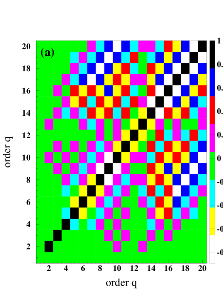
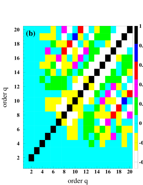
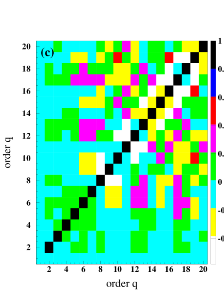
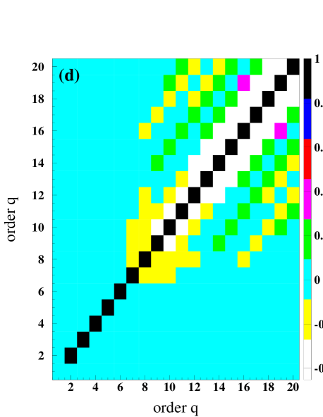
Figure 6.2: Correlation matrices of $H_{q}$ obtained from samples generated according to a Poisson distributions with $1\cdot 10^{5}$ events (a), $5\cdot 10^{5}$ events (b), $1\cdot 10^{6}$ events (c) and $2\cdot 10^{9}$ events (d).

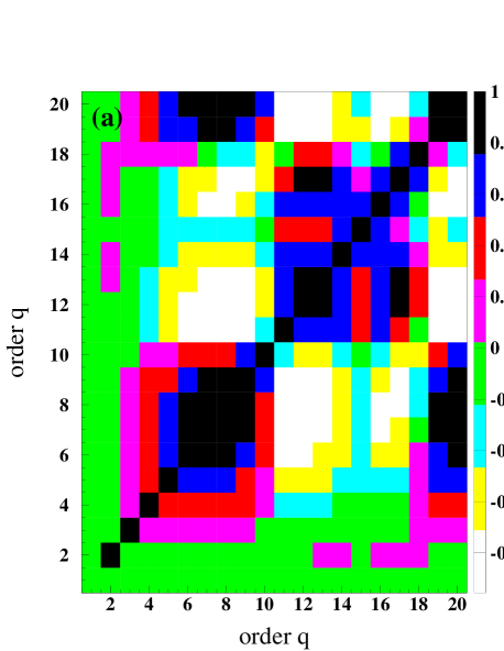
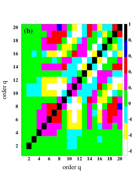
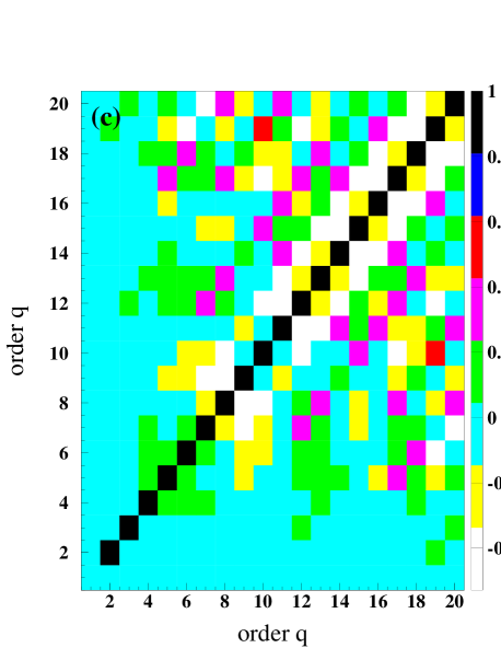
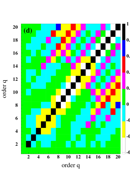
Figure 6.3: Effect of statistical fluctuation on the $H_{q}$ correlation matrices obtained from various 1-million event samples generated according to a Poisson distribution. In (a) 2 events have been added at large multiplicities, in (b) only one, (c) none and (d) the distribution of (c) is truncated.

6.1.2 $H_{q}$ and truncation

The first truncation we should talk about, as an experimentalist, is the truncation in the tail of the charged-particle multiplicity distribution as a consequence of the finite statistics of our samples. In any experimental multiplicity distribution, there is a maximum multiplicity $n_{\text{max}}$ above which no events are seen. Therefore, we should rewrite Eq. (1.3), the mathematical definition of the factorial moment $F_{q}$ in a more experimental way:

$$F_{q}=\frac{\overset{n_{\text{max}}}{\underset{n=q}{\sum}}n(n-1)....(n-q+1)P(n)}{\overset{n_{\text{max}}}{\underset{n=q}{\sum}}nP(n)},$$ (6.1)

where $n_{\text{max}}$ is the largest multiplicity obtained for a given sample. But we should also worry about the significance of high multiplicities which lack precision, as seen in Fig. 4.4 and Table 4.7 for the full sample where $\text{K}^{0}_{\text{s}}$ and $\Lambda$ are assumed to be stable. Multiplicities larger than 48 have relative errors larger than $78\%$, which clearly means that the knowledge we have of these multiplicities is almost non-existent. They are statistical fluctuations, their presence or their absence does not have any real physical meaning, and hence they should be removed. Although their impact on the measurement of the mean of the charged-particle multiplicity distribution is negligible, this is not the case for the measurement of the $H_{q}$ moments. Previous analyses have shown [46] that the $H_{q}$ moments are very sensitive to the truncation of the tail of the charged-particle multiplicity distribution. This sensitivity comes from the definition of the factorial moment, $F_{q}$ (Eq. (6.1)). For example, if we impose a truncation at $n_{\text{max}}-1$, we can write for the non-normalized factorial moments,

$$\tilde{F}_{q}=\overset{n_{\text{max}}-1}{\underset{n=q}{\sum}}\frac{n!}{(n-q)!}P(n)+\frac{n_{\text{max}}!}{(n_{\text{max}}-q)!}P(n_{\text{max}}),$$ (6.2)

and we see that the importance of the last term rises with the order $q$. Thus, we see that a statistical fluctuation at very high multiplicity can have an important influence on the final result. Since the $H_{q}$ measurement is expected to perform a detailed analysis of the shape of the charged-particle multiplicity distribution, such a high multiplicity statistical fluctuation can destroy or mask part of the information we want to gather. Therefore, multiplicities which can be considered as dominated by statistical fluctuations must be removed from the sample for the $H_{q}$ analysis. These multiplicities are characterized by the instability of their values and, hence, have very large relative error. In Fig. 4.4, we noticed a large change in the relative error between $n=48$ ($29\%$) and $n=50$ ($78\%$). Therefore, it seems reasonable to remove multiplicities larger than 48. These relative errors, which take into account both statistical and systematic errors, allow to take into account both aspects of the statistical fluctuation at high multiplicities, one being due to, stricto sensus, the statistics, the other due to the sensitivity to the choice of selection criteria of high multiplicity “boundary” events.

The problem of sensitivity of the $H_{q}$ to the truncation of the tail of the multiplicity distribution is not limited to multiplicities which are largely dominated by statistical fluctuations, they are only the most astonishing example of this effect. As we know from the above preliminary study of the $H_{q}$, truncating statistical fluctuation is fully justified by the fact that it removes correlations introduced by such events, but we also know that truncating meaningful information will introduce even further correlations. Anyhow, the truncation will always have an influence on the result. Contrary to the study in the previous sub-section, which was performed on a Poisson distribution, we cannot predict the theoretical behavior of the experimental charged-particle multiplicity distribution. Therefore, we cannot precisely quantify the bias of the $H_{q}$ introduced by the use of the truncated distribution. To limit this bias, the truncation must be limited to the elimination of multiplicities which are sensitive to large statistical fluctuations.

The effects of the truncation are shown in Fig. 6.4, where the reference $H_{q}$ sample (in which multiplicities influenced by large statistical fluctuations are removed) for the full sample without $\text{K}^{0}_{\text{s}}$ and $\Lambda$ decay products is compared to the same distribution where no truncation has been applied (Fig. 6.4(a)) and where the distribution has been exaggeratedly truncated (Fig. 6.4(b)), removing multiplicities known with a rather good accuracy (and therefore assumed to be statistically significant). At low $q$, we can also note an improvement of the statistical error, obtained by removing multiplicities having large statistical error (and hence being influenced by statistical fluctuation).

Figure 6.4: (a) Comparison between the reference $H_{q}$ moment (coming from the full sample truncated at $n=48$) and $H_{q}$ moment obtained from the distribution before applying the truncation, (b) for a strongly truncated (at $n=44$) distribution. Only statistical errors are shown.

The effect of the truncation being part of our measurement, we have to make sure that all distributions we want to compare are affected by the truncation in the same way. Therefore, it is not possible to express the truncation as a fixed cut on the multiplicity distribution. It is very unlikely that the sensitivity to statistical fluctuation of the multiplicities larger than 48 is the same for the full sample without and with $\text{K}^{0}_{\text{s}}$ and $\Lambda$ decay products. The second distribution contains the same events, for which the $\text{K}^{0}_{\text{s}}\text{ and }\Lambda$ have been allowed to decay. These events are found to have on average two more charged particles than in the first place. In other words, the multiplicity distribution can be described, in first approximation, as shifted by about 2 particles. So are the statistical fluctuations. Therefore, in order to remove these events in both distributions, we remove the tail of the second charged-particle multiplicity distribution which corresponds to the fraction of events removed by a truncation at 48 in the first.

Because of rather long lifetimes of $\text{K}^{0}_{\text{s}}\text{ and }\Lambda$’s, their decays take place at the end of the chain of processes leading to the final state. Therefore, the $q$-particle correlations in which their decay products (not the $\text{K}^{0}_{\text{s}}\text{ and }\Lambda$ themselves, which are already taken into account) are involved are certainly limited to their closest neighbors in momentum space. Therefore, it is reasonable to expect correlations only between a small number of particles. In terms of $q$-particle correlation functions, this means that the $H_{q}$ moments obtained from the two distributions, with and without $\text{K}^{0}_{\text{s}}\text{ and }\Lambda$ decay products, should have rather similar values, except at low $q$ (small changes are nevertheless expected as a consequence of the correlation between the $H_{q}$ moments, which were found to be rather small in the previous section).

This is illustrated in Figs. 6.6 and 6.6, where we compare the full sample with and without $\text{K}^{0}_{\text{s}}$ and $\Lambda$ decay products. When we apply a truncation at $n=48$ for both distributions, the two distributions disagree. However, if the fraction of events corresponding to a truncation on multiplicities larger than 48 for the full sample where $\text{K}^{0}_{\text{s}}$ and $\Lambda$ are stable is removed from the full sample including $\text{K}^{0}_{\text{s}}$ and $\Lambda$ (which corresponds to a truncation on multiplicities larger than 52) we have good agreement between the two samples.

Now, if we apply the inverse, we fix the truncation on the multiplicity at $n=48$ for the full sample where the $\text{K}^{0}_{\text{s}}$ and $\Lambda$ decay products are taken into account and remove the corresponding fraction in the other sample (which corresponds to a truncation on multiplicities larger than 44) we also have a good agreement between the two distributions. This shows us (apart from the fact that the weakly decaying short life-time particles don’t have any influence on the shape of the charged-particle multiplicity distribution) that we have to define the truncation in terms of an equal fraction of events to be removed in the tail of the multiplicity distribution.

Only $0.005\%$ of the events are in fact removed by this truncation.

We have seen in this sub-section that the amplitude of the oscillation is increased by the truncation, thereby amplifying an already existing behavior. This is due to an increase in the size of the correlations between $H_{q}$, which then amplifies the original $H_{q}$. On the other hand, statistical fluctuation destroying the original correlation pattern will partly mask the original $H_{q}$ behavior as seen in the previous sub-section. This is illustrated in Fig. 6.4(a), where the original data sample, having large statistical fluctuation in its tail, has much smaller oscillations than the truncated one. Since the statistical fluctuation masks the oscillatory behavior, the fact that we have small oscillation strongly suggests that the oscillatory behavior is not due to the truncation. Nevertheless, too strong truncation may increase the oscillation size. This is illustrated in Fig. 6.4 (b), where we have applied a truncation removing well measured and hence statistically significant multiplicities and the size of the oscillation is increased.

Figure 6.5: Comparison between the full samples without and with $\text{K}^{0}_{\text{s}}$ and $\Lambda$ decay products, (a) where the truncation has removed multiplicities larger than 48 and (b) where the truncation has removed the fraction of events defined by a truncation on multiplicities larger than 48 on the full sample without $\text{K}^{0}_{\text{s}}$ and $\Lambda$ decay products. Only statistical errors are shown.

Figure 6.6: Comparison between the full samples without and with $\text{K}^{0}_{\text{s}}$ and $\Lambda$ decay products where the truncation has removed the fraction of events defined by a truncation on multiplicities larger than 44 on the full sample without $\text{K}^{0}_{\text{s}}$ and $\Lambda$ decay products, corresponding to the truncation of multiplicities larger than 48 for the full sample including decay products of $\text{K}^{0}_{\text{s}}$ and $\Lambda$. Only statistical errors are shown.

6.1.3 Statistical errors

The statistical errors on the $H_{q}$ are obtained by two different methods: The first one, an analytical method, which we prefer, is error propagation, making use of the covariance matrix of the charged-particle multiplicity distribution. The dependence of our estimate of the covariance matrix on the statistics, together with the form of the derivative of the $H_{q}$ moments, which can emphasize even small changes in the covariance matrix, causes this method to give reliable results only for high-statistics samples. At low statistics, the approximations and assumptions used to estimate the covariance matrix are not valid anymore. Since it would be rather difficult to obtain a better estimate of the covariance matrix, a Monte Carlo based method is found to be a rather advantageous alternative of treating the error, all terms being naturally taken into account by this method. Therefore, the analytical method is used for the full and the light-quark samples where large statistics makes it suitable, but the second method will be used for the b-quark sample, which has smaller statistics.

Analytical method

In this method, the statistical errors are obtained by error propagation, which makes use of the covariance matrix of the charged-particle multiplicity distribution, $\text{CoV}(P(i),P(j))$. The variance of the $H_{q}$, $\text{Var}(H_{q})$, is given by

$$\text{Var}(H_{q})={\underset{i,j}{\sum}}\frac{\partial H_{q}}{\partial P(i)}\frac{\partial H_{q}}{\partial P(j)}\text{CoV}(P(i),P(j)),$$ (6.3)

where $\frac{\partial H_{q}}{\partial P(i)}$ is a partial derivative of $H_{q}$ as a function of the multiplicity $P(i)$. These terms can be easily obtained by writing $H_{q}$ as a function of the non-normalized factorial moment $\tilde{F_{q}}$ corresponding to:

$$\tilde{F_{q}}=\overset{n_{\text{max}}}{\underset{n=q}{\sum}}n(n-1)....(n-q+1)P(n)=F_{q}\tilde{F_{1}}^{q}.$$ (6.4)

It must be noted that $\tilde{F_{1}}$ is nothing but the mean of the multiplicity distribution. Dividing the cumulant factorial moment, $K_{q}$, (Eq. (1.4)) by $F_{q}$, we can express $H_{q}$ as a sum of factorial moments:

$$H_{q}=1-\overset{q-1}{\underset{m=1}{\sum}}\frac{(q-1)!}{m!(q-m-1)!}H_{q-m}\frac{F_{q-m}F_{m}}{F_{q}}\text{ with }H_{1}=F_{1}=1.$$ (6.5)

We see also that the normalization factor of the factorial moments, corresponding to the mean of the multiplicity distribution cancels, leading to

$$H_{q}=1-\overset{q-1}{\underset{m=1}{\sum}}\frac{(q-1)!}{m!(q-m-1)!}H_{q-m}\frac{\tilde{F}_{q-m}\tilde{F}_{m}}{\tilde{F}_{q}}.$$ (6.6)

Therefore, the derivative of $H_{q}$ is given by

$$\text{d}H_{q}=-\overset{q-1}{\underset{m=1}{\sum}}\frac{(q-1)!}{m!(q-m-1)!}H_{q-m}\frac{\tilde{F}_{q-m}\tilde{F}_{m}}{\tilde{F}_{q}}(\frac{\text{d}H_{q-m}}{H_{q-m}}+\frac{\text{d}\tilde{F}_{q-m}}{\tilde{F}_{q-m}}+\frac{\text{d}\tilde{F}_{m}}{\tilde{F}_{m}}-\frac{\text{d}\tilde{F}_{q}}{\tilde{F}_{q}}),$$ (6.7)

$$\text{where }\text{d}\tilde{F}_{q}=\begin{cases}n(n-1)....(n-q+1)\text{d}P(n)&n\geq q\\ 0&n<q.\end{cases}$$ (6.8)

The first non-zero partial derivative, $\frac{\partial H_{2}}{\partial P(n)}$, obtained from Eqs. (6.7) and (6.8) is given by:

$$\frac{\partial H_{2}}{\partial P(n)}=(H_{2}-1)\large\begin{cases}\frac{2n}{\tilde{F}_{1}}-\frac{n(n-1)}{\tilde{F}_{2}}&n\geq 2\\ \frac{2n}{\tilde{F}_{1}}&n=1.\end{cases}$$ (6.9)

The partial derivatives of the higher $H_{q}$ moments are found iteratively, starting with the $H_{2}$ partial derivative, $\frac{\partial H_{2}}{\partial n}$ in Eq. (6.7).

This way of calculating statistical errors works well, unless the sample size becomes too small. Samples which have less than 500.000 events cannot be processed by this method. At that point, the combination of the deterioration in the precision of the covariance matrix, together with the higher-order terms of the $H_{q}$ derivative, cause the resulting statistical error to significantly deviate from its real value and become larger. In order to obtain a reliable estimation, we need to take into account all orders of correlation. It would be very difficult to do this analytically. Therefore, we use a Monte Carlo based method.

Monte Carlo based error calculation

The principle of this method is very simple. A large number of multiplicity distributions are generated from the experimental one by allowing random variation of the multiplicities which compose it. Each of these generated multiplicity distributions gives an $H_{q}$ value. The error is then extracted from the distribution of the generated $H_{q}$.

In order to generate a multiplicity distribution as close as possible to the experimental result, the generation process has to follow the same treatment and reconstruction process as used for the experimental data. Since events are produced independently of each other, the random variation of the multiplicity distribution is obtained by imposing Poisson fluctuation of the number of events produced with a given multiplicity.

The generation process starts by imposing a Poisson fluctuation on the number of events for each detected multiplicity $N^{\text{raw}}(i)$ of the data. This allows us to calculate a completely new (but statistically consistent with the original distribution) probability distribution, $P^{\text{raw}}_{1}(i)$.

Next, making use of the detector response matrix, $\mathcal{M}$ , we impose a Poisson fluctuation on the number of events $N(n_{\text{det}},n_{\text{prod}})$ with $n_{\text{det}}$ detected particles and $n_{\text{prod}}$ produced tracks. We then obtain not only a completely new detector response matrix $\mathcal{M}_{1}$ but also new Monte Carlo produced and detected multiplicity distributions, $P_{1}(n_{\text{prod}})$ and $P_{1}(n_{\text{det}})$.

We then perform a reconstruction of the new data distribution, $P^{\text{raw}}_{1}(i)$, by the Bayesian unfolding method making use of the newly obtained probability matrix $\mathcal{M}_{1}$. A reconstructed charged-particle multiplicity distribution of the data, $P^{\text{data}}_{1}(n_{\text{prod}})$, is obtained. This distribution has, of course, to be corrected, like the normal data sample, for event selection, initial-state radiation, $\text{K}^{0}_{\text{s}}$ and $\Lambda$ decay products, light- or b-quark purities. Since all these corrective factors have a statistical influence on the final result, Poisson fluctuations of the number of events of each multiplicity are also imposed on all the multiplicity distributions which compose them. We finally get a completely new fully reconstructed and corrected multiplicity distribution, $P^{\text{data}}_{1}(n_{\text{prod}})$, from which a new set of $H^{(1)}_{q}$ moments is calculated. The whole operation is then repeated 1000 times, in order to obtain $H^{(i)}_{q}$ distributions. After having checked that the distributions of $H^{(i)}_{q}$ are close to Gaussian (see Fig. 6.7 as examples) centered around the original $H_{q}$ measurement, the statistical error on the $H_{q}$ is taken to be the half-width of the distribution.

Figure 6.7: Distributions of the $H_{2}$, (a), and $H_{8}$, (b), obtained after the generation of 10.000 distributions.

Figure 6.8: $H_{q}$ moments for light-quark sample (a) and b-quark sample (b). The error lines is for the statistical error calculated by the analytical method, the error boxes for the statistical errors calculated with the Monte Carlo based method.

Since this procedure is rather time consuming, the number of generated multiplicity distributions is chosen in such a way that the precision of the error ( the error on the error) is sufficiently accurate. For 1000 multiplicity distributions, the error is known within an accuracy of $3.2\%$, which is sufficiently small. (For comparison, the error committed by giving the value of the mean charged-particle multiplicity of the b-quark sample with a precision of 0.01 is $16\%$). Furthermore, in view of the size of the systematic error, which is always the major contribution to the error in this analysis, the accuracy of $3.2\%$ for the statistical error is fine. A comparison between the analytical method and this method given in Fig. 6.8, shows both the limitation of the analytical method at low statistics and the advantage of the use of the analytical method. For the light-quark sample (Fig. 6.8(a)) where the statistics is high (about 1,200.000 events after corrections), the two methods give the same results, but for the b-quark sample, where the statistics is smaller (about 300.000 events after corrections), the analytical method, which is not able to insure a proper cancellation of the correlations introduced by the reduction of the statistics, largely overestimates the statistical errors on the $H_{q}$.

6.1.4 Systematic errors

The estimation of the systematic errors is based on the systematic study of the charged-particle multiplicity distribution described in Sect. 4.3, where we have determined charged-particle multiplicity distributions corresponding to the various checks of systematic effects. Here, we determine the $H_{q}$ moments from these distributions. The resulting $H_{q}$ moments are then compared to the $H_{q}$ moments of the reference sample in the same way as was described in Sect. 4.3, replacing the charged-particle multiplicity distributions by the $H_{q}$ moments. Contributions to the systematic errors are then due to the track quality cuts, which are again the largest contribution, the event selection, uncertainties in Monte Carlo modelling, the unfolding method used to reconstruct the charged-particle multiplicity distribution, and the light- or b-tagging method.

6.2 Results for the full, light- and b-quark samples

The $H_{q}$ moments are measured for the full, light-quark and b-quark samples without and with $\text{K}^{0}_{\text{s}}\text{ and }\Lambda$ decay products. They are shown as a function of the order $q$ in Figs. 6.9, 6.10 and 6.11, together with $H_{q}$ moments calculated from charged-particle multiplicity distributions obtained from events generated with JETSET, ARIADNE and HERWIG. The size of the Monte Carlo samples is similar to that of the data, except for JETSET which contains 3 times more events. For all the data samples, the $H_{q}$ moments exhibit a first negative minimum at $q=5$ and quasi-oscillation for higher $q$. While JETSET and ARIADNE show relatively good agreement for all the samples, the $H_{q}$ moments calculated from events generated with HERWIG do not agree with any of them. For all samples, they show a shift of at least one order for all extrema. Furthermore, the $H_{q}$ obtained for the HERWIG full and light-quark samples, have amplitudes of oscillation which are much larger than those found in the data. For the b-quark sample, apart from the one-order shift of the extrema, the amplitudes of the oscillation have about the size of those of the data.

Figure 6.9: $H_{q}$ as a function of $q$ for the full samples (a) without and (b) with $\text{K}^{0}_{\text{s}}\text{ and }\Lambda$ decay products, together with JETSET, HERWIG and ARIADNE.

Figure 6.10: $H_{q}$ as a function of $q$ for the light-quark samples (a) without and (b) with $\text{K}^{0}_{\text{s}}\text{ and }\Lambda$ decay products, together with JETSET, HERWIG and ARIADNE.

Figure 6.11: $H_{q}$ as a function of $q$ for the b-quark samples (a) without and (b) with $\text{K}^{0}_{\text{s}}\text{ and }\Lambda$ decay products, together with JETSET, HERWIG and ARIADNE.

Figure 6.12: $H_{q}$ as a function of $q$ for the full, light- and b-quark samples (a) without and (b) with $\text{K}^{0}_{\text{s}}\text{ and }\Lambda$ decay products.

In Fig. 6.12, we can see that the full, light- and b-quark samples agree well with each other, with only a small difference for small $q$ ($q<5$), between the b-quark sample and the other samples. This indicates that the weak decay of the b quark does not have much influence on the shape of the charged-particle multiplicity distribution. It must be noted that neither does the weak decay of $\text{K}^{0}_{\text{s}}\text{ and }\Lambda$ have much influence on the shape of the multiplicity distribution.

The $H_{q}$ behavior observed for the data is qualitatively similar to that predicted by the NNLLA assuming Local Parton-Hadron Duality. However, also JETSET agrees well with all the data samples (and HERWIG, even if it does not agree with the data, predicts the same kind of features, a first negative minimum followed by quasi-oscillation). However, none of the parton showers used by those Monte Carlo models have implemented NNLLA. Rather, they use parton showers which are close in form to the MLLA with, in addition, full energy-momentum conservation.

Therefore, we attempt to find which aspect of the Monte Carlo generation is responsible for this agreement.

6.3 Monte Carlo analysis of the $H_{q}$

In view of the good agreement of JETSET with the data for all samples, we vary several options in JETSET and study their influence on the shape of the charged-particle multiplicity distribution and hence, on the $H_{q}$ behavior.

Since analytical QCD predicts the $H_{q}$ behavior for partons, we tried first to change in JETSET, options related to the parton production, keeping in all cases the Lund string fragmentation model for the hadronization. We try the following:

• No angular ordering in the parton shower. This makes it essentially an LLA shower with, in addition, energy-momentum conservation. Removing this constraint allows more partons to be generated. Therefore, the multiplicity distribution generated that way should have a larger average number of particles and should be broader.

• Partons are generated according to $\mathcal{O}(\alpha_{\text{s}})$ and $\mathcal{O}(\alpha^{2}_{\text{s}})$ matrix elements and even only $\text{q}\bar{\text{q}}$. Since only a small number of partons are generated under these models, the charged-particle multiplicity distribution has smaller mean and dispersion.

Figure 6.13: $H_{q}$ moment of the full sample, together with events generated with JETSET (a) using a LLA parton shower, (b) using $\mathcal{O}(\alpha^{2}_{\text{s}})$ matrix element, (c) using $\mathcal{O}(\alpha^{1}_{\text{s}})$ matrix element and (d) generating a $\text{q}\bar{\text{q}}$ pair only, and in all cases the Lund string fragmentation.

For all four cases ( multiplicity distribution generated with Lund string fragmentation and partons according LLA parton shower, $\mathcal{O}(\alpha^{2}_{\text{s}})$, $\mathcal{O}(\alpha^{1}_{\text{s}})$, and $\text{q}\bar{\text{q}}$ only), we find that the $H_{q}$ moments calculated from the corresponding charged-particle multiplicity distribution, have a first negative minimum around $q=5$ followed by quasi-oscillations as is seen in Fig. 6.13. Even though, these various models do not reproduce the $H_{q}$ behavior exactly, we find qualitative agreement with the $H_{q}$ oscillatory behavior seen in the data. The matrix element models have slightly smaller oscillation size than the parton shower models. We notice that the depth of the first negative minimum decreases with decreasing matrix element order. Also the amplitudes of the oscillation are smaller for the distributions generated with partons according matrix elements, but it must be noted that these distributions contain fewer particles than those generated according to the parton shower implementation.

This shows us that the overall features of the $H_{q}$ behavior do not depend on a particular model for the generation of partons.

The next step is to consider that the oscillatory behavior may originate from the fragmentation, which could simulate some higher-order aspects of pQCD. Therefore, we repeat the previous study, replacing the Lund string model by the independent fragmentation model. We also allow in both Lund string and independent fragmentation models, resonances to decay. As a further test, we split the samples into light- and b-quark samples.

For the full samples (Fig. 6.14), most of what we try gives oscillations of about the size of the data. However, the $H_{q}$ moments obtained with a LLA parton shower and independent fragmentation (with and without resonances) shows a different behavior. It has a first negative minimum at $q=4$ and, instead of smooth oscillation for higher $q$, the $H_{q}$ moment oscillates with a short period. In this particular case, the combination of the LLA parton shower and independent fragmentation models gives birth to a very wide distribution with a dispersion near 10 and a mean of the charged-particle multiplicity distribution of about 30.

Figure 6.14: $H_{q}$ moment of the full sample compared to events generated (a) using LLA parton shower, (b) with $\mathcal{O}(\alpha^{2}_{\text{s}})$ matrix element, (c) $\mathcal{O}(\alpha_{\text{s}})$ matrix element and (d) only $\text{q}\bar{\text{q}}$ for various fragmentation options.

Also for the light-quark samples (Fig. 6.15) we obtain for most of the samples $H_{q}$ moments which have a first negative minimum for $q$ between 4 and 6 and oscillatory behavior for larger $q$, but these oscillations are usually smaller. More specifically, the $H_{q}$ moments generated from distributions obtained with LLA parton shower and independent fragmentation, without resonance decays shows a first negative minimum at 4 followed by a positive maximum at 5 and small oscillation. With resonance decays, we have a similar behavior but shifted by one order. For only $\text{q}\bar{\text{q}}$ with both string and independent fragmentation without resonance decay, we cannot see any oscillation but some erratic behavior. This seems to be related to the absence of the resonances, since the model using independent fragmentation with resonances shows the oscillatory behavior.

Figure 6.15: $H_{q}$ moment of the light-quark sample compared to events generated (a) using LLA parton shower, (b) with $\mathcal{O}(\alpha^{2}_{\text{s}})$ matrix element, (c) $\mathcal{O}(\alpha_{\text{s}})$ matrix element and (d) only $\text{q}\bar{\text{q}}$ for various fragmentation options.

Figure 6.16: $H_{q}$ moment of the b-quark sample compared to events generated (a) using LLA parton shower, (b) with $\mathcal{O}(\alpha^{2}_{\text{s}})$ matrix element, (c) $\mathcal{O}(\alpha_{\text{s}})$ matrix element and (d) only $\text{q}\bar{\text{q}}$ for various fragmentation options.

Figure 6.17: $H_{q}$ moment of the full sample compared to that of parton distributions obtained at 91  and at 910 .

For the b-quark sample (Figs. 6.16), all the charged-particle multiplicity distributions give $H_{q}$ moments for which oscillatory behavior is seen. Except for the LLA parton shower, which has a large amplitude compared to the data, the charged-particle multiplicity distributions for which partons have been generated using matrix elements have relatively small oscillations.

Most of the models we have checked show a first negative minimum at about $q=5$, followed by an oscillatory behavior qualitatively similar to the one seen in the data, no matter which model is used to generate the partons and for most of the options we tried for the fragmentation.

Concerning the absence of $H_{q}$ oscillation in some samples, this cannot be related to a specific aspect of the fragmentation. The two charged-particle multiplicity distributions in question concern completely different, even opposite, models. One generating partons according to LLA showers, the other using only $\text{q}\bar{\text{q}}$. Furthermore, in the first case the two models which do not have oscillation are those using independent fragmentation with and without resonance. But in the second case, it is both string and independent fragmentation without resonances which do not show the oscillation.

As an additional test, we also determined the $H_{q}$ moments of the parton multiplicity distribution instead of the charged-particle multiplicity distribution. This test was performed on the default parton shower of the JETSET model at the center-of-mass energy of 91 and of 910 . The resulting $H_{q}$ moments are shown in Fig. 6.17 together with that of the data. We see that the $H_{q}$ moments obtained from the partons at the $\mathrm{Z}^{0}$ energy do not present the usual oscillatory behavior but has an erratic behavior. However its first negative minimum is at $q=6$. At 910 , for which the parton multiplicity distribution has about the same mean as the mean charged-particle multiplicity at the $\mathrm{Z}^{0}$ energy, the $H_{q}$ moments display an oscillatory behavior having about the same amplitude as the data, but shifted by one order.

It seems that there is no particular aspect of the Monte Carlo responsible for the presence or the absence of the $H_{q}$ oscillatory behavior, but that it is due to a collective effect, various aspects of the Monte Carlo contributing to the oscillations in various models. From this Monte Carlo study, even if we fail in finding a unique origin for these oscillations, we can nevertheless conclude that these oscillations can be reproduced without the need of NNLLA of perturbative QCD.

Therefore, in the next chapter, we will attempt to challenge more directly perturbative QCD, by measuring the $H_{q}$ moments for the jet multiplicity distribution at energy scales where pQCD is the dominant mechanism.

Chapter 7 Analysis of jet multiplicity distributions with the $H_{q}$

In the previous chapter, we compared the $H_{q}$ moments of the charged-particle multiplicity distribution with various analytical QCD predictions and in particular with the NNLLA predictions. Originally applying to partons, these predictions are made valid for final-state particles by the use of the Local Parton-Hadron Duality (LPHD) assumption. This assumption may be summarized from our point of interest as the hypothesis that the shape of the partonic distribution is not distorted by the hadronization. Therefore, the $H_{q}$ moments obtained for the partonic distribution should be similar to those of the final-state particle multiplicity distribution and, by extension, to those of the charged-particle multiplicity distribution. Therefore, the comparison of the $H_{q}$ moments of the charged-particle multiplicity distribution to the pQCD prediction rests strongly on the validity of LPHD.

In order to remove the dependence on LPHD, we use the jet multiplicity distribution instead of the charged-particle multiplicity distribution. Since jets obtained for an energy scale above 1-2  fall into the domain of validity of pQCD, they correspond to partons.

In the first section, the various steps needed to measure the jet multiplicity distributions are briefly described, as well as the estimation of statistical and systematic errors. The next section is dedicated to the measurement of the $H_{q}$ moments for a wide range of energy scales above and below the 1  limit of the perturbative QCD region. The results are compared to analytical QCD expectations.

7.1 Experimental procedures

The jet multiplicity distribution is defined as the distribution of the number of jets reconstructed from an event at a given energy scale. These jets are built with the Durham algorithm [47] using charged particles only. This has the advantage that the jet multiplicity distribution obtained with $y_{\text{cut}}$ near zero corresponds to the charged-particle multiplicity distribution. Since most of the comparison is done relative to the charged-particle multiplicity distribution, we know that for very small $y_{\text{cut}}$ values, the jet multiplicity distribution will approach the charged-particle multiplicity distribution.

The main disadvantage is that the method does not use the full event, but only charged particles. This may affect the number of reconstructed jets. The effect will increase with decreasing value of $y_{\text{cut}}$ (the effect will be maximal for $y_{\text{cut}}$=0 where each particle is resolved as a jet). However, particles are distributed in such a way that, at energy scales close to the domain of validity of pQCD, the number of reconstructed jets does not depend too much on the fact that we use only the charged particles. Furthermore, since our main interest is the shape of the distribution, it does not really matter that we use the charged-particle multiplicity distribution instead of the multiplicity distribution of all particles. Both distributions have equivalent shape. Therefore, even for low $y_{\text{cut}}$ where the bias is maximum, the difference will not be large.

Using the Durham algorithm, the cut-off parameter value $y_{\text{cut}}$ defines a jet energy scale which is closely related to the transverse energy $E^{\text{jet}}_{\text{t}}$ of the jet,

$$E^{\text{jet}}_{\text{t}}=E_{\text{cm}}\sqrt{y_{\text{cut}}},$$ (7.1)

where $E_{\text{cm}}$ is the center-of-mass energy of the collision. Therefore, in this chapter we will preferably refer to the jet energy scale, $E^{\text{jet}}_{\text{t}}$, rather than to the cut-off parameter $y_{\text{cut}}$. Nevertheless, Table 7.1 shows the correspondence between the two parameters.

$y_{\text{cut}}$	$1.2\cdot 10^{-6}$	$2.7\cdot 10^{-6}$	$4.8\cdot 10^{-6}$	$7.5\cdot 10^{-6}$	$1.1\cdot 10^{-5}$	$1.9\cdot 10^{-5}$
$E^{\text{jet}}_{\text{t}}$ ()	0.1	0.15	0.2	0.25	0.3	0.4
$y_{\text{cut}}$	$3\cdot 10^{-5}$	$4.3\cdot 10^{-5}$	$1.2\cdot 10^{-4}$	$3.9\cdot 10^{-4}$	$8.2\cdot 10^{-4}$	$1.1\cdot 10^{-3}$
$E^{\text{jet}}_{\text{t}}$()	0.5	0.6	1	1.8	2.6	3

Table 7.1: Correspondence between the jet energy scale $E^{\text{jet}}_{\text{t}}$ and the cut-off parameter $y_{\text{cut}}$.

From the range of energy resolution given in Table 7.1, we are able to follow in great detail the evolution of partons into hadrons, and hence we should be able to match any change in the behavior of the $H_{q}$ moments to any phase which could occur in the evolution of partons into hadrons.

The jet multiplicity distributions are reconstructed in exactly the same way as the charged-particle multiplicity distribution. The only difference is that we build the distribution of the number of events with $n_{\text{jet}}$ jets, $N(n_{\text{jet}})$, instead of the distribution of the number of events with $n$ charged-particles, $N(n)$. As for the charged-particle multiplicity distribution, these distributions are corrected for detector inefficiencies by the Bayesian unfolding method. They are also corrected for the selection procedures and initial-state radiation using bin-by-bin correction factors. Since the $H_{q}$ of the light- and b-quark samples are found to agree with the $H_{q}$ of the full sample, only results for the full sample are shown. Further, we limit our study to the case where $\text{K}^{0}_{\text{s}}\text{ and }\Lambda$ are assumed to be stable.

The estimation of both statistical and systematic errors follows the same procedures as already used for the charged-particle multiplicity distribution. In the estimation of the systematic errors we include contributions from changing the track quality criteria and the event selection, from the influence of the unfolding method and also a contribution coming from Monte Carlo modelling uncertainties.

Furthermore, in the determination of the $H_{q}$ moments from the jet multiplicity distributions, we use the same criteria for the truncation as used for the charged-particle multiplicity distribution (, we remove in the jet multiplicity distributions the same fraction of events as removed by a cut on multiplicities larger than 48 in the charged-particle multiplicity distribution of the full sample). In this way we are able to directly compare the $H_{q}$ moments obtained from the jet multiplicity distributions to those obtained from the charged-particle multiplicity distribution of the full sample. To estimate the statistical errors on the $H_{q}$ moments, we use the Monte Carlo based method described in the previous chapter. The systematic errors of the $H_{q}$ moments are obtained in the usual way.

7.2 $H_{q}$ moments of the jet multiplicity distributions

The $H_{q}$ moments determined from the jet multiplicity distributions are shown in Figs. 7.1 to 7.3, for the $y_{\text{cut}}$ values given in Table 7.1. For $E^{\text{jet}}_{\text{t}}$=100  (Fig. 7.1(a)), the $H_{q}$ moments show a first negative minimum at $q=5$ and oscillatory behavior for larger vales of $q$. This behavior is similar to that observed for the charged-particle multiplicity distribution, but the oscillations are smaller in amplitude. By increasing the energy resolution of the jet algorithm, the amplitude of the oscillation decreases further. At $E^{\text{jet}}_{\text{t}}$=200  (Fig. 7.1(c)), the first negative minimum has shifted to $q=4$, the oscillation has disappeared for $q>8$ and is much reduced between $q=6$ and $q=8$. Between $E^{\text{jet}}_{\text{t}}$=200  and $E^{\text{jet}}_{\text{t}}$=300  (Fig. 7.2(a)), the first negative minimum at $q=4$ deepens sharply. The same sharp decrease is also seen for $q=2$ in the insert. For $q>6$, $H_{q}$ remains as it was at lower energy scales. At $E^{\text{jet}}_{\text{t}}$=400  (Fig. 7.2(b)), a new first minimum appears at $q=2$ with a much deeper value than for $q=4$, and for $q<5$ $H_{q}$ alternates between positive and negative values. For larger $q$ values, the $H_{q}$ remain roughly constant about 0.

At $E^{\text{jet}}_{\text{t}}$=500  (Fig. 7.2(c)), we have a complete change of the $H_{q}$: the smooth quasi-oscillations we see for the lowest energy scales have disappeared and $H_{q}$ alternates between positive and negative values for all $q$. We notice also that this sign-changing behavior has an amplitude almost twice as large as than at $E^{\text{jet}}_{\text{t}}$=400 . As we increase the energy scale further, there is no noticeable change in the $H_{q}$ with respect to $E^{\text{jet}}_{\text{t}}$=500 . The only difference is that the absolute value of each $H_{q}$ has increased. At $E^{\text{jet}}_{\text{t}}$=1  (Fig. 7.3(a)), we enter the domain of validity of the perturbative region and the behavior is similar to that already observed for $E^{\text{jet}}_{t}>500~{}\MeV{}$, but the amplitude is much larger.

It seems that the increase in the scale of the $H_{q}$ values is due to the decrease of the mean jet multiplicity. Increasing the energy scale further does not bring anything new. We still have the sign-changing behavior as we already observed, but again the $H_{q}$ moments have greater values.

In these figures we also find an overall good agreement with JETSET. HERWIG is seen to disagree with the data at small energy scales ($E^{\text{jet}}_{t}<250~{}\MeV{}$). Nevertheless, this disagreement diminishes with the increase of the energy scale, and for larger energy scales and in particular in the perturbative region, HERWIG agrees well with the data.

Figure 7.1: $H_{q}$ moments of jet multiplicity distribution obtained with (a) $E^{\text{jet}}_{\text{t}}$=100 , (b) $E^{\text{jet}}_{\text{t}}$=150 , (c) $E^{\text{jet}}_{\text{t}}$=200  and (d) $E^{\text{jet}}_{\text{t}}$=250 .

Figure 7.2: $H_{q}$ moments of jet multiplicity distribution obtained with (a) $E^{\text{jet}}_{\text{t}}$=300 , (b) $E^{\text{jet}}_{\text{t}}$=400 , (c) $E^{\text{jet}}_{\text{t}}$=500  and (d) $E^{\text{jet}}_{\text{t}}$=600 .

Figure 7.3: $H_{q}$ moments of jet multiplicity distribution obtained with (a) $E^{\text{jet}}_{\text{t}}$=1 , (b) $E^{\text{jet}}_{\text{t}}$=1.8 ,(c) $E^{\text{jet}}_{\text{t}}$=2.6  and (d) $E^{\text{jet}}_{\text{t}}$=3 .

Figure 7.4: Evolution of $H_{2}$, (a), $H_{3}$, (b), $H_{6}$, (c), and $H_{13}$, (d), with the jet energy scale.

We can summarize the evolution of the $H_{q}$ behavior with the energy scale in three main steps. At low energy scale, $E^{\text{jet}}_{\text{t}}<200~{}\MeV{}$, the $H_{q}$ behavior is qualitatively similar to that of the charged-particle multiplicity distribution, with a first negative minimum around $q=5$ and oscillatory behavior for larger values of $q$. The second step, $200~{}\MeV{}<E^{\text{jet}}_{\text{t}}<500~{}\MeV{}$, can be described as a transition phase where the oscillation disappears and a first negative minimum appears at $q=2$. Finally, in the third step, $E^{\text{jet}}_{\text{t}}>500~{}\MeV{}$, a completely different behavior is observed where the $H_{q}$ alternates between negative and positive values.

The details of this evolution are easier to see, in particular for the transition phase, when the $H_{q}$ is plotted as a function of $E^{\text{jet}}_{\text{t}}$. Fig. 7.4(b) illustrates the beginning of the transition phase. It is characterized by the appearance of a minimum at $E^{\text{jet}}_{\text{t}}$=200  in $H_{3}$, which also marks the end of the step of the $H_{q}$ oscillatory behavior similar to that of the charged-particle multiplicity distribution. Fig. 7.4(a) represents the evolution of $H_{2}$ with the energy scale and illustrates one of the major changes in the $H_{q}$ behavior which occurs during the transition phase. This is the appearance of the first negative minimum at $q=2$ and the first sign of the sign changing $H_{q}$ behavior which characterize the $H_{q}$ at large $E^{\text{jet}}_{\text{t}}$and in the perturbative region. Fig. 7.4(c) shows the evolution of $H_{6}$ with the energy scale. We can see that all the transition phase is located around the maximum value. The end of this transition phase and the beginning of the full sign-changing $H_{q}$ behavior at large $q$ is easily seen, $H_{13}$ in Fig. 7.4(d). The whole transition phase is characterized by a plateau where $H_{13}$ has a stable value near 0, up to an energy scale of $500\MeV$.

7.3 Comparison with theoretical expectations

Assuming that the $H_{q}$ behavior is described by analytical QCD, then we should expect to find this behavior for partons. Assuming that the jets correspond to the partons, we should find the $H_{q}$ behavior predicted for partons for the jets produced at an energy scale of 1-2 . But as we have discussed above, in the perturbative region we see a sign-changing $H_{q}$ behavior which is not described by any of the analytical QCD predictions, and in particular is not described by the NNLLA.

The oscillatory behavior appears only in the final stages of the hadronization process, far away from the perturbative region. Therefore, it is not possible to link this oscillatory behavior to the NNLLA. We can conclude that the $H_{q}$ oscillatory behavior observed for the charged-particle multiplicity distribution and for jet multiplicity distributions obtained at very low energy scales has no relation with the $H_{q}$ behavior predicted by the NNLLA.

Chapter 8 2- and 3-jet event multiplicity distributions

In search of an alternative way of describing the shape of the charged-particle multiplicity distribution, we test, in this chapter, phenomenological approaches [29, 30] by making use of the charged-particle multiplicity distributions of the 2-jet and 3-jet events taken from the full sample, as well as the light- and b-quark samples. Two main approaches are tested experimentally in this chapter:

In the first one, we assume that the dominant influence on the shape of the charged-particle multiplicity distribution of the full sample comes from the jet configuration of the events. Assuming that the charged-particle multiplicity distribution of both the 2-jet and the 3-jet events can be described by a negative binomial distribution, the full sample would be described by a weighted sum of the negative binomial distributions of the 2-jet and 3-jet events [29]. (We first assume here that we have only 2-jet and 3-jet events, the 3-jet events being the events which are not classified as 2-jet events). The parametrization describing the full sample would then be

$$f_{\text{full}}(n)=R_{2}f^{\text{NB}}_{\text{2-jet}}(n,\langle n_{2}\rangle,k_{2})+(1-R_{2})f^{\text{NB}}_{\text{3-jet}}(n,\langle n_{3}\rangle,k_{3}),$$ (8.1)

where the parameter of the NBDs are found from the means and dispersions measured from the experimental charged-particle multiplicity distribution of these two samples. A previous analysis [48] found it possible to describe simultaneously the charged-particle multiplicity distributions 2-, 3- and 4-jet events by NBDs for certain $y_{\text{cut}}$ values of the JADE algorithm. This gave credit to this approach.

As an extension, we also investigate this approach for the charged-particle multiplicity distributions of the light- and b-quark samples, assuming they can be related in the same way as the full sample to the jet configurations of their events.

The second approach relies on the flavor composition of the full sample. It assumes that both the charged-particle multiplicity distributions of the 2-jet and the 3-jet events can be described by a weighted sum of negative binomial distributions related to the flavor composition of these 2-jet and 3-jet events [30].

$$f_{\text{2,3-jet}}(x)=R_{\text{b}}f^{\text{NB}}_{\text{2,3-jet light-quark}}(x,\langle n_{\text{light}}\rangle,k_{\text{light}})+(1-R_{\text{b}})f^{\text{NB}}_{\text{2,3-jet b-quark}}(x,\langle n_{\text{b}}\rangle,k_{\text{b}}),$$ (8.2)

where $R_{\text{b}}$ is the relative hadronic cross section of the b-quark system.

This hypothesis is also tested on the full sample, trying in this case to parametrize it using negative binomial distribution to describe individually the charged-particle multiplicity distributions of the light- and b-quark samples.

In order to test all these hypotheses, we decompose the full, light- and b-quark samples into 2-jet and 3-jet events obtained for different values of the cut-off parameter $y_{\text{cut}}$ of the Durham algorithm. Their corresponding charged-particle multiplicity distributions are then reconstructed and used to calculate the means and dispersions which are used as parameters of the NBD parametrizations.

In the first section, we describe briefly the various steps needed to reconstruct the charged-particle multiplicity distributions of the 2-jet and 3-jet events. In the next section, we present the determination of the moments (including the $H_{q}$ moments) of the 2-jet and 3-jet events obtained from the full, light- and b-quark samples. In the penultimate section, the two phenomenological approaches are confronted with the experimental results discussed. Finally, in the last section, we present an extension of the phenomenological approaches, by decomposing the full sample into well defined jet topologies such as pencil-like 2-jet and Mercedes-like 3-jet events with, in addition, the remaining events coming from 3-jet events having a softer gluon jet. This approach seems to explain the origin of the $H_{q}$ oscillatory behavior of the charged-particle multiplicity distribution of the full sample, as due to the diversity of jet topologies and hard gluon radiation which coexist at the $\mathrm{Z}^{0}$ energy.

8.1 Experimental procedures

In this section are briefly summarized all the procedures needed for our measurements. Since most of the corrections and error estimations have already been discussed in previous chapters, the various steps needed for the present measurements will be just indicated.

The classification into 2-jet and 3-jet events is achieved using the Durham jet algorithm. We define as 2-jet event, an event which has been classified at a given value of the cut-off parameter, $y_{\text{cut}}$ as 2-jet event. Events not classified as 2-jet are called 3-jet.

Since the charged particles represent only a fraction of the particles produced (and of the energy radiated) during an collision, it is preferable, as we do, to apply the jet algorithm to the whole event and not only to charged particles. While most of the events are not affected by this change, some of the events, having $y_{\text{23}}$ values ($y_{\text{23}}$ is the value of $y_{\text{cut}}$ for which a 2-jet event becomes a 3-jet event) close to the $y_{\text{cut}}$ value used for a particular 2-jet definition, will be rather sensitive to whether the neutral particles are included in the jet algorithm.

Once the event has been classified as a 2- or 3-jet event, its number of charged particles is extracted. The charged-particle multiplicity distributions of the 2- or 3-jet events are then built from the distribution of the number of charged particles in the same way as in the previous chapters. Also reconstruction and corrections as well as the estimation of the statistical and systematic errors are identical (see Chapter 4 for more details).

In order to have a more flexible definition of 2-jet events and to avoid any strong dependence, in our analysis, on a particular $y_{\text{cut}}$ value, we use six different values of the cut-off parameter. This also enables us to study the evolution of the the charged-particle multiplicity distribution with the cut-off parameter. The six $y_{\text{cut}}$ values have been chosen such that both the 2-jet and the 3-jet sub-samples always have enough statistics to allow simultaneously both types analyses. The fraction of 2-jet events, $R_{2}$, obtained for the $y_{\text{cut}}$ values used in our analysis are given in Table 8.1 for the full, light- and b-quark samples, respectively. While, in general, we observe rather similar 2-jet fraction for the full, light- and b-quark samples for each $y_{\text{cut}}$, we see a depletion in 2-jet events obtained with $y_{\text{cut}}$=0.002 for the b-quark sample. This may be explained by some mis-assignment between 2-jet and 3-jet events due to the weak decay of the b quark at such a low $y_{\text{cut}}$ value.

$y_{\text{cut}}$	full sample	light-quark sample	b-quark sample
0.030	$82.0\%$	$81.2\%$	$83.0\%$
0.015	$71.5\%$	$71.1\%$	$73.3\%$
0.010	$64.6\%$	$64.1\%$	$66.7\%$
0.006	$55.1\%$	$54.6\%$	$57.0\%$
0.004	$46.5\%$	$46.4\%$	$46.8\%$
0.002	$29.3\%$	$31.3\%$	$22.0\%$

Table 8.1: Fraction of 2-jet events, $R_{2}$, for the full, light- and b-quark samples obtained for the 6 $y_{\text{cut}}$ values used in this analysis.

The fully corrected charged-particle multiplicity distributions of the 2- and 3-jet events obtained from the full, light- and b-quark samples are then used for our analysis. We restrict the analysis to the charged-particle multiplicity distributions where $\text{K}^{0}_{\text{s}}\text{ and }\Lambda$ are considered stable.

Since the fraction of identified 2- or 3-jet events varies with the cut-off parameter value, $y_{\text{cut}}$, it is interesting to link this number of reconstructed jets to the number of primary partons. To check that, we use Monte Carlo events generated in a relatively simple case. We use JETSET to generate events according to the $\mathcal{O}(\alpha_{\text{s}})$ matrix element followed by the Lund string fragmentation. In this simple case, the particles produced in the final state come from a maximum of 3 partons. We use the Durham algorithm with the same $y_{\text{cut}}$ values used in our analysis to reconstruct jets from the final-state particles and we compare the result to the number of initial partons generated by JETSET. Fig. 8.2 shows the fraction of events with 2- and 3-parton final states which have been identified as 2- or 3-jet events by the jet algorithm.

We first note that the 2-parton events represent only a small fraction ($16\%$) of the events. We find that these events are almost always reconstructed as 2-jet events by the jet-algorithm for the range of $y_{\text{cut}}$ used in the analysis even for small $y_{\text{cut}}$ values. At $y_{\text{cut}}$=0.002, the fraction of events mistaken as 3-jet events is only $1.6\%$. For this $y_{\text{cut}}$ value about $80\%$ of the 3-parton events are identified as 3-jet, however this fraction will decrease when the $y_{\text{cut}}$ value will be increased. The remaining 3-parton events correspond to pencil-like events accompanied by a very low transverse momentum gluon, collinear to the quark-jet direction. These events cannot be identified as 3-jet events by the jet algorithm even at very low $y_{\text{cut}}$ value. Using a value smaller than 0.002 would increase the fraction of 2-parton events mistaken as 3-jet but would not have any effect in reducing the fraction of 3-parton events mistaken as 2-jet events. Therefore, changing the $y_{\text{cut}}$ value will act only on the identification of 3-parton events as 2- or 3-jets. By changing the $y_{\text{cut}}$ value, we mainly change the “hardness” criterion of the primary gluon. This is illustrated in Fig. 8.2, which shows the transverse momentum of the gluon in 3-parton events which have been identified as 2-jets at the different $y_{\text{cut}}$ values. Since the cut-off parameter of the Durham algorithm is linked to the transverse momentum of the jet, the gluon will be considered part of the quark jet if the transverse momentum of the gluon is smaller than $E_{\text{cms}}\sqrt{y_{\text{cut}}}$. Therefore, the jet configuration depends mainly on the hardness of the primary gluon.

Figure 8.1: Fraction of events generated with JETSET $\mathcal{O}(\alpha_{\text{s}})$ with 2 or 3 partons and classified as 2- or 3-jet.

Figure 8.2: Transverse momentum of the gluon jet in JETSET $\mathcal{O}(\alpha_{\text{s}})$ 3-parton events classified as 2-jet events for several $y_{\text{cut}}$ values.

8.2 Moments of the 2- and 3-jet events

Examples of charged-particle multiplicity distributions measured for 2-jet and 3-jet events are shown in Fig. 8.3(a) and (b) for the full sample with $y_{\text{cut}}$=0.03 and $y_{\text{cut}}$=0.01, in Fig. 8.5 for the light-quark sample with $y_{\text{cut}}$=0.006 and in Fig. 8.5 for the b-quark sample with $y_{\text{cut}}$=0.004. We note that JETSET agrees with the data in all cases, but HERWIG shows large disagreement for high multiplicities in the 2-jet events of all samples. The agreement is rather good for the 3-jet events of the full sample and of the light-quark sample, but it is bad for the b-quark sample.

We determined the mean, $\langle n\rangle$, and the dispersion, $D$, for all the 2- and 3-jet event charged-particle multiplicity distributions. They are given in Table 8.2 for the 2-jet events and in Table 8.3 for the 3-jet events.

Figure 8.3: Charged-particle multiplicity distributions of 2-jet and 3-jet events obtained from the full sample with (a) $y_{\text{cut}}$=0.03 and (b) $y_{\text{cut}}$=0.01.

Figure 8.4: Charged-particle multiplicity distributions of 2-jet and 3-jet events obtained from the light-quark sample with $y_{\text{cut}}$=0.006.

Figure 8.5: Charged-particle multiplicity distributions of 2-jet and 3-jet events obtained from the b-quark sample with $y_{\text{cut}}$=0.004.

		full sample	light-quark sample	b-quark sample
$0.03$	$\langle n\rangle$	$17.51\pm 0.01\pm 0.08$	$16.95\pm 0.01\pm 0.07$	$19.44\pm 0.02\pm 0.11$
	$D$	1$5.24\pm 0.01\pm 0.04$	1$5.10\pm 0.01\pm 0.04$	1$5.15\pm 0.01\pm 0.04$
$0.015$	$\langle n\rangle$	$16.94\pm 0.01\pm 0.07$	$16.36\pm 0.01\pm 0.07$	$18.90\pm 0.02\pm 0.10$
	$D$	1$4.95\pm 0.01\pm 0.04$	1$4.80\pm 0.01\pm 0.04$	1$4.88\pm 0.02\pm 0.03$
$0.01$	$\langle n\rangle$	$16.57\pm 0.01\pm 0.07$	$15.99\pm 0.01\pm 0.06$	$18.55\pm 0.02\pm 0.10$
	$D$	1$4.78\pm 0.01\pm 0.03$	1$4.62\pm 0.01\pm 0.04$	1$4.71\pm 0.02\pm 0.03$
$0.006$	$\langle n\rangle$	$16.07\pm 0.01\pm 0.07$	$15.48\pm 0.01\pm 0.06$	$18.07\pm 0.01\pm 0.09$
	$D$	1$4.56\pm 0.01\pm 0.03$	1$4.39\pm 0.01\pm 0.03$	1$4.48\pm 0.03\pm 0.03$
$0.004$	$\langle n\rangle$	$15.62\pm 0.01\pm 0.06$	$15.04\pm 0.01\pm 0.06$	$17.64\pm 0.01\pm 0.09$
	$D$	1$4.38\pm 0.01\pm 0.03$	1$4.20\pm 0.01\pm 0.04$	1$4.33\pm 0.03\pm 0.04$
$0.002$	$\langle n\rangle$	$14.65\pm 0.01\pm 0.06$	$14.21\pm 0.01\pm 0.05$	$16.90\pm 0.01\pm 0.08$
	$D$	1$4.07\pm 0.01\pm 0.04$	1$3.90\pm 0.01\pm 0.05$	1$4.12\pm 0.06\pm 0.05$

Table 8.2: Mean $\langle n\rangle$ and dispersions $D$ of the 2-jet events.

		full sample	light-quark sample	b-quark sample
$0.03$	$\langle n\rangle$	$23.74\pm 0.02\pm 0.13$	$23.14\pm 0.02\pm 0.12$	$25.80\pm 0.09\pm 0.15$
	$D$	1$5.96\pm 0.01\pm 0.07$	1$5.83\pm 0.02\pm 0.08$	1$5.81\pm 0.05\pm 0.05$
$0.015$	$\langle n\rangle$	$22.91\pm 0.01\pm 0.12$	$22.32\pm 0.01\pm 0.12$	$24.97\pm 0.06\pm 0.15$
	$D$	1$5.89\pm 0.01\pm 0.07$	1$5.75\pm 0.01\pm 0.07$	1$5.75\pm 0.04\pm 0.06$
$0.01$	$\langle n\rangle$	$22.41\pm 0.01\pm 0.13$	$21.82\pm 0.01\pm 0.12$	$24.48\pm 0.05\pm 0.16$
	$D$	1$5.85\pm 0.01\pm 0.06$	1$5.71\pm 0.01\pm 0.07$	1$5.71\pm 0.04\pm 0.06$
$0.006$	$\langle n\rangle$	$21.79\pm 0.01\pm 0.13$	$21.22\pm 0.01\pm 0.12$	$23.77\pm 0.05\pm 0.15$
	$D$	1$5.81\pm 0.01\pm 0.06$	1$5.67\pm 0.01\pm 0.07$	1$5.71\pm 0.03\pm 0.06$
$0.004$	$\langle n\rangle$	$21.28\pm 0.01\pm 0.14$	$20.74\pm 0.01\pm 0.13$	$23.06\pm 0.04\pm 0.15$
	$D$	1$5.77\pm 0.01\pm 0.06$	1$5.64\pm 0.01\pm 0.06$	1$5.71\pm 0.03\pm 0.05$
$0.002$	$\langle n\rangle$	$20.31\pm 0.01\pm 0.14$	$19.86\pm 0.01\pm 0.13$	$21.54\pm 0.03\pm 0.16$
	$D$	1$5.74\pm 0.01\pm 0.06$	1$5.62\pm 0.01\pm 0.06$	1$5.77\pm 0.02\pm 0.06$

Table 8.3: Mean $\langle n\rangle$ and dispersion $D$ of the 3-jet events.

We further determined the $H_{q}$ moments for the 2- and 3-jet events in the full, light- and b-quark samples. We used the same truncation criteria as in the previous chapters. A comparison between the $H_{q}$ for the full sample and the $H_{q}$ for the 2-jet and 3-jet events obtained from the full sample with a $y_{\text{cut}}$=0.015 is given in Fig. 8.7. It shows that even the largest $H_{q}$ oscillations obtained from any 2- or 3-jet event samples (what we see in Fig. 8.7 for $y_{\text{cut}}$=0.0015 is also true for any other $y_{\text{cut}}$) are much smaller than those in the full sample.

Fig. 8.8 shows the $H_{q}$ moments for 2- and 3-jet events obtained from the full sample for the 6 $y_{\text{cut}}$ values. For the 2-jet events we find that the size of the oscillations decreases with decreasing $y_{\text{cut}}$. For $y_{\text{cut}}$=0.030, where the 2-jet fraction represents $82\%$ of the full sample and can include rather broad 2-jet events, the oscillations have about half the amplitude of those of the full sample. They further decrease gradually until $y_{\text{cut}}$=0.004, where the oscillations have almost completely disappeared.

For the 3-jet events, we have the opposite trend. For $y_{\text{cut}}$=0.03 and $y_{\text{cut}}$=0.015, the $H_{q}$ moments do not show any oscillation. As $y_{\text{cut}}$ decreases, the amplitude of the oscillation increases to reach about half the size of those of the full sample at $y_{\text{cut}}$=0.002.

We must also note that the absence of oscillations in the 2-jet samples and in the 3-jet samples are obtained for completely different jet configurations. The low $y_{\text{cut}}$ values for which the absence of oscillation occurs for 2-jet events, identify as 2-jet events only those events which have narrow jets, almost back to back (pencil-like 2-jet events). For the 3-jet events, it is for large $y_{\text{cut}}$values that the oscillations disappear. For these $y_{\text{cut}}$ values, the events selected as 3-jet can have a very broad jet configuration, and hence they have a configuration close to the Mercedes-like 3-jet events. In both configurations, the energy is shared almost equally among the jets.

We also measure the $H_{q}$ moments of the charged-particle multiplicity distributions of the 2-jet and 3-jet events obtained from the light- and b-quark samples. The $H_{q}$ behavior does not exhibit any significant difference from that of the $H_{q}$ moments derived from the 2- and 3-jet events obtained from the full sample. Two examples are given in Fig. 8.9 for the light-quark sample and two in Fig. 8.10 for the b-quark sample. The major differences, we found, are confined to low $q$ values ($q<5$). This is further illustrated in Fig. 8.7, where $H_{2}$ and $H_{6}$ are plotted as a function of $y_{\text{cut}}$ for the 2- and 3-jet events obtained from the light- and b-quark samples. For $H_{2}$, we see a rather large difference for both 2- and 3-jet between the light- and b-quark samples, while for $H_{6}$, differences between light- and b-quark samples have almost disappeared.

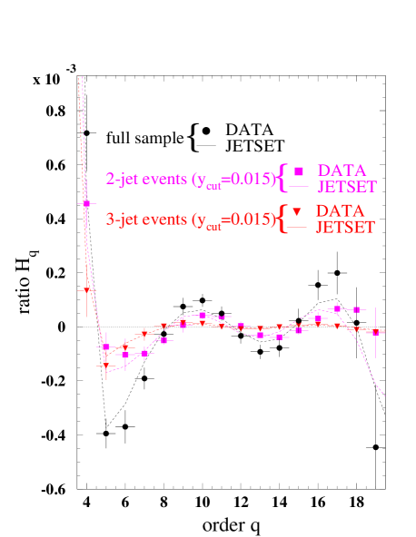
Figure 8.6: $H_{q}$ moments of the full sample and and of 2- and 3-jet events obtained with $y_{\text{cut}}$=0.015.

Figure 8.7: $H_{2}$ (top plot) and $H_{6}$ (bottom plot) plotted versus $y_{\text{cut}}$ for 2- and 3-jet obtained from both light- and b-quark samples.

Figure 8.8: $H_{q}$ moments measured from the charged-particle multiplicity distributions of the 2- and 3-jet of the full sample for (a) $y_{\text{cut}}$=0.03, (b) $y_{\text{cut}}$=0.015, (c) $y_{\text{cut}}$=0.01, (d) $y_{\text{cut}}$=0.006, (e) $y_{\text{cut}}$=0.004 and (f) $y_{\text{cut}}$=0.002.

Figure 8.9: $H_{q}$ moments measured from the charged-particle multiplicity distributions of the 2- and 3-jet in the light-quark sample for (a) $y_{\text{cut}}$=0.015 and (b) $y_{\text{cut}}$=0.002.

Figure 8.10: $H_{q}$ moments measured from the charged-particle multiplicity distributions of the 2- and 3-jet in the b-quark sample for (a) $y_{\text{cut}}$=0.03 and (b) $y_{\text{cut}}$=0.004.

8.3 The phenomenological approach

This approach views the shape of charged-particle multiplicity distribution of the full sample as the result of the superposition of distributions originating from various processes related to the topology of the events, , 2-jet and 3-jet or light-quark and heavy-quark events. Assuming that each of these processes can be described by a relatively simple parametrization such as the NBD, the charged-particle multiplicity distribution of the full sample would then be a weighted sum of all the contributions. Altogether, these various contributions would explain the shape of the charged-particle multiplicity distribution and ultimately its $H_{q}$ behavior. In the framework of this approach, we investigate two hypotheses. In the first hypothesis we assume that the shape of the charged-particle multiplicity distribution of the full sample arises from the superposition of 2-jet and 3-jet events [29]. In the second hypothesis we assume that the full sample and also those of the 2-jet and the 3-jet events can be parametrized by superposition of flavor related distributions [30].

8.3.1 2- and 3-jet superposition

In this hypothesis we assume that the main features of the shape of the charged-particle multiplicity distribution of full, light- and b-quark samples responsible for the oscillatory behavior of the $H_{q}$ moments, can be described by a weighted sum of two NBDs (Eq. (8.1)), the two NBDs themselves describing the charged-particle multiplicity distributions of the 2-jet and of the 3-jet events, respectively. The parameters of the 2 NBD’s are obtained from the experimental charged-particle multiplicity distributions of the 2-jet and 3-jet events (Tables 8.2 and 8.3 for the 2-jet and the 3-jet events, respectively), the weight between the 2 NBD’s is taken as the 2-jet fraction obtained for a given $y_{\text{cut}}$ value (Table 8.1). This fraction can also be calculated from the means of the charged-particle multiplicity distributions of the 2-jet, 3-jet events and of the full samples.

We first compare the data and the single NBDs, $f_{\text{2-jet}}^{\text{NB}}(n,\langle n_{2}\rangle,k_{2})$ and $f_{\text{3-jet}}^{\text{NB}}(n,\langle n_{3}\rangle,k_{3})$ where the parameters $\langle n_{2,3}\rangle$ and $k_{2,3}$ are taken from the experimental 2- and 3-jet charged-particle multiplicity distributions according to Eq. (1.9). The corresponding $\chi^{2}$ confidence levels are given in Table 8.4. We find good agreement for the 2-jet events obtained for $y_{\text{cut}}$ smaller than 0.01. We note also that the agreement increases gradually with decreasing $y_{\text{cut}}$ value.

For the 3-jet events, , non-2-jet events, we observe the opposite of what is observed for the 2-jet events. The agreement with the single-NBD parametrization improves with increasing $y_{\text{cut}}$ value. We have good agreement with the charged-particle multiplicity distribution of the 3-jet events for $y_{\text{cut}}$ values larger than 0.06.

A few examples of the single-NBD parametrization, together with the charged-particle multiplicity distributions of 2-jet events and of 3-jet events are given in Figs. 8.14, 8.14 and 8.16 for the full, light- and b-quark samples, respectively. The same behavior is observed in the same proportion for the full, light- and b-quark samples. It seems there is a strong relation between the agreement with the single-NBD expectation and the jet configuration of the events.

For the 2-jet events we see that agreement is obtained at low $y_{\text{cut}}$ values. For these values, the jet algorithm resolves fewer and fewer events as 2-jet events, which means that the remaining 2-jet events have a less ambiguous 2-jet status than those of the previous ones (these events have relatively narrow jets, and may be described as pencil-like 2-jet events).

For the 3-jet events, the agreement with the single-NBD is obtained at large $y_{\text{cut}}$ value. This means that the fraction of events not considered as 2-jet events is small and these events have topologies very different from the 2-jet topologies (they are close to Mercedes-like 3-jet events). Thus, agreement with a single-NBD is obtained for events which have completely different jet configurations and also completely different charged-particle multiplicity distributions, namely pencil-like 2-jet and Mercedes-like 3-jet events. This would suggest that the mixture of jet configurations plays an important role in the origin of the oscillatory behavior of the $H_{q}$, since the $H_{q}$ moments obtained from the charged-particle multiplicity distributions of these jet configurations themselves (multiplicity distributions obtained from 2-jet with $y_{\text{cut}}$ smaller than 0.006 and 3-jet with $y_{\text{cut}}$ larger than 0.01) do not show this oscillatory behavior (Fig. 8.8). This will be discussed in more detail in the next section.

Although we both conclude that the jet configuration plays an important role, what we find is rather in contradiction with DELPHI analysis [48]. This collaboration claimed good agreement between charged-particle multiplicity distributions and the single-NBD parametrization simultaneously for the 2-jet, 3-jet and 4-jet obtained at the same $y_{\text{cut}}$. This is never the case in our analysis, since where there is good agreement with the 2-jet events, there is poor agreement for the 3-jet events (and vice versa).

Next, we compare the charged-particle multiplicity distribution of the full, light- and b-quark samples with the distribution $f_{\text{full}}(x,y_{\text{cut}})$ obtained from the weighted sum of the two NBDs (Eq. (8.1)), one corresponding to the charged-particle multiplicity distribution of the 2-jet events, the other to the 3-jet events both obtained at the same $y_{\text{cut}}$ value. This procedure gives us a fully constrained two-NBD parametrization of the charged-particle multiplicity distributions. The $\chi^{2}$ confidence levels are given in Table 8.5.

We find an overall good agreement between these two-NBD parametrizations and the charged-particle multiplicity distribution of the full, light- and b-quark samples. The charged-particle multiplicity distributions of the full, light- and b-quark samples are shown in Figs. 8.14,  8.14 and 8.16, together with the parametrizations for various values of $y_{\text{cut}}$. This agreement is also reflected in the $H_{q}$. The $H_{q}$ calculated from the two-NBD parametrization is seen to agree quite well with the data for the full sample as well as for both light- and b-quark samples, as seen in Figs. 8.14,  8.14 and 8.16, respectively.

Figure 8.11: Charged-particle multiplicity distributions of the full sample and of 2-jet and 3-jet events obtained with $y_{\text{cut}}$=0.01 fitted by various two-NBD and single-NBD parametrizations, respectively.

Figure 8.12: $H_{q}$ moments of the full sample, together with the $H_{q}$ moments calculated from the two-NBD parametrization.

Figure 8.13: Charged-particle multiplicity distributions of the light-quark sample and of 2-jet and 3-jet events obtained with $y_{\text{cut}}$=0.01 fitted by various two-NBD and single-NBD parametrizations, respectively.

Figure 8.14: $H_{q}$ moments of the light-quark sample, together with the $H_{q}$ moments calculated from the two-NBD parametrization.

Figure 8.15: Charged-particle multiplicity distributions of the b-quark sample and of 2-jet and 3-jet events obtained with $y_{\text{cut}}$=0.01 fitted by various two-NBD and single-NBD parametrizations, respectively.

Figure 8.16: $H_{q}$ moments of the b-quark sample, together with the $H_{q}$ moments calculated from the two-NBD parametrization.

This agreement is rather odd since, as we have seen previously, for a given $y_{\text{cut}}$ value, only one of the two distributions can be well described by a NBD. Therefore, we cannot conclude that the two-NBD hypothesis in terms of 2-jet and non-2-jet events is a success.

However, as we cannot claim the success of this two-NBD parametrization, we cannot ignore that very singular jet configurations as the ones observed above are well described by a single-NBD parametrization. This gives some indication of where the aspect of the charged-particle multiplicity distribution, responsible for the oscillatory behavior of the $H_{q}$, might lie. We have already identified two (non overlapping) components of the charged-particle multiplicity distribution which do not have this oscillatory behavior. As it will be discussed later in this chapter, the answer might lie in the multijet part of the charged-particle multiplicity distribution which is ignored in this parametrization, so far.

	full sample		light-quark sample		b-quark sample
$y_{\text{cut}}$	2-jet event	3-jet event	2-jet event	3-jet event	2-jet event	3-jet event
$0.03$	$10^{-6}$	0.89	$10^{-9}$	0.90	$10^{-8}$	0.94
$0.015$	$10^{-4}$	0.34	$10^{-6}$	0.36	$10^{-6}$	0.60
$0.01$	0.002	0.02	$10^{-3}$	0.04	$10^{-4}$	0.21
$0.006$	0.42	$10^{-5}$	0.11	$10^{-4}$	0.34	0.05
$0.004$	0.83	$10^{-9}$	0.65	$10^{-8}$	0.49	$10^{-4}$
$0.002$	0.82	$10^{-14}$	0.97	$10^{-13}$	0.81	$10^{-5}$

Table 8.4: $\chi^{2}$ confidence level between the NBD parametrization and their experimental counterpart.

$y_{\text{cut}}$	full sample	light-quark sample	b-quark sample
$0.03$	0.04	$10^{-3}$	$10^{-3}$
$0.015$	0.57	0.19	0.15
$0.01$	0.74	0.42	0.56
$0.006$	0.48	0.19	0.86
$0.004$	0.03	0.01	0.54
$0.002$	$10^{-12}$	$10^{-11}$	$10^{-4}$

Table 8.5: $\chi^{2}$ confidence level between the 2-jet, 3-jet parametrizations and their experimental counterpart.

8.3.2 Light- and b-quark superposition

Instead of viewing the origin of the main features of the shape and of the $H_{q}$ oscillatory behavior of the charged-particle multiplicity distribution of the full sample as due to the superposition of the 2-jet and 3-jet events, the other hypothesis relates these features to the flavor content of the sample [30].

Therefore, with this hypothesis, we attempt to describe the charged-particle multiplicity distributions of the 2-jet events and the 3-jet events of the full sample themselves as a weighted sum of two NBDs, using parameters taken from the charged-particle multiplicity distribution of the 2-jet (or 3-jet) events of the light- and b-quark samples (Eq. (8.2)). Knowing that the $H_{q}$ moments of the full, light- and b-quark samples have oscillations of about the same size (see Fig. 6.12), as it is the case for 2-jet and 3-jet obtained from the full, light- and b-quark samples, we can also test, as a consistency check, this hypothesis on the full sample.

Results are summarized in Table 8.6 for the charged-particle multiplicity distributions of the 2-jet and 3-jet events.

$y_{\text{cut}}$	2-jet events	3-jet events
$1$	$1\cdot 10^{-18}$
$0.03$	$8\cdot 10^{-12}$	0.56
$0.015$	$2\cdot 10^{-9}$	0.04
$0.01$	$1\cdot 10^{-5}$	$2\cdot 10^{-4}$
$0.006$	0.01	$8\cdot 10^{-8}$
$0.004$	0.24	$3\cdot 10^{-12}$
$0.002$	$7\cdot 10^{-5}$	$1\cdot 10^{-16}$

Table 8.6: $\chi^{2}$ confidence level between the charged-particle multiplicity distributions of the 2-jet, 3-jet events of the full sample and the light, b-quark parametrization.

The parametrization of the charged-particle multiplicity distributions of the 2-jet and 3-jet events are mainly found to be in disagreement with the data, except for the 2-jet sample for $y_{\text{cut}}$=0.006 and $y_{\text{cut}}$=0.004. But this seems to be more related to the fact that for these $y_{\text{cut}}$ values, the 2-jet or 3-jet events of the full sample are already described by single-NBDs (see Table 8.4).

The parametrization of the charged-particle multiplicity distribution of the full sample by two NBD’s representing the light- and b-quark contributions is found not to describe the data ($\chi^{2}$ confidence level of $1\cdot 10^{-18}$). Therefore, the shape of the charged-particle multiplicity distribution of the full sample, or even of the 2- and 3-jet events cannot be described in terms of light- and b-quark superposition. Examples of that were already given in terms of the $H_{q}$ moments for the full, light- and b-quark samples (Fig. 6.12 in Chapter 6) and for the 2-jet and 3-jet samples in Fig. 8.7, which show that the oscillatory behavior is very similar for the three samples. We can deduce from that, that if there is a phenomenon responsible for the oscillations, it plays the same role in the full sample as in both light- and b-quark samples and consequently cannot be due to the flavor composition of the sample.

8.4 Origin of the $H_{q}$ oscillatory behavior

In the previous sections, we found that extreme 2- or 3-jet configurations did not show the $H_{q}$ oscillatory behavior seen in the full sample and that they were quite well described by single NBD’s.

Since both these extreme 2- and 3-jet configurations co-exist in the full sample, in this section, we try to isolate simultaneously these configurations from the full sample. As seen in the Monte Carlo study at parton level in the previous section, the remaining events, which can neither be categorized, undoubtfully, as 2-jet nor as 3-jet events, can be identified as 3-jet events where the third jet is a gluon-jet with energy smaller than that of the two quark-jets. In the following, we will call these events, soft-jet events.

Following Eq. (1.6), we can write the charged-particle multiplicity distribution in terms of these three components as

$$P(n)=R_{2}(y_{\text{2-jet}})P_{\text{2-jet}}(n)+R_{3}(y_{\text{3-jet}})P_{\text{3-jet}}(n)+(1-R_{2}(y_{\text{3-jet}})-R_{2}(y_{\text{2-jet}}))P_{\text{soft-jet}}(n),$$ (8.3)

where the $P_{\text{2-jet}}(n)$, $P_{\text{3-jet}}(n)$ and $P_{\text{soft-jet}}(n)$ are the charged-particle multiplicity distributions of the extreme 2- and 3-jet events and of the soft-jet events, respectively. $R_{2}(y_{\text{2-jet}})$ and $R_{3}(y_{\text{3-jet}})$ are the rate of the 2-jet and 3-jet events obtained for the $y_{\text{cut}}$ values $y_{\text{2-jet}}$ and $y_{\text{3-jet}}$, respectively.

The charged-particle multiplicity distribution of the soft-jet events is reconstructed from events remaining once we have identified the 2-jet and 3-jet events having charged-particle multiplicity distributions which do not show the $H_{q}$ oscillatory behavior. From our choice of $y_{\text{cut}}$, we use for the pencil-like 2-jet events the charged-particle multiplicity distributions obtained with $y_{\text{cut}}$=0.004 or $y_{\text{cut}}$=0.002. For the Mercedes-like 3-jet events, the charged-particle multiplicity distributions are obtained with $y_{\text{cut}}$=0.03 or $y_{\text{cut}}$=0.015. Therefore, we have four different possible charged-particle multiplicity distributions for soft-jet events. These distributions are corrected and reconstructed in the same way as any other distributions used in this analysis. The production rates, means and dispersions of the charged-particle multiplicity distributions of soft-jet events are given in Table 8.7. We also include, the $\chi^{2}$ confidence levels of the comparison of the charged-particle multiplicity distribution with the single-NBD. The agreement is rather bad, except for the case with $y_{\text{cut}}$ values of 0.004 and 0.015, respectively. As an extension to the phenomenological approach tested in the previous section, we also test for this case the agreement between charged-particle multiplicity distribution of the full sample and its parametrization obtained by the use of 3 NBD’s describing the 2-, 3- and soft-jet events, as given in Eq. (1.7). With a $\chi^{2}$ confidence level of 0.96, the three-NBD parametrization is found to be in very good agreement with the charged-particle multiplicity distribution of the full sample.

Also the $H_{q}$ moments of the soft-jet charged-particle multiplicity distributions are determined. They are shown together with the $H_{q}$ moments of the 2-jet and 3-jet events in Fig. 8.17. We see that the amplitudes of the oscillations are comparable to the residual oscillations seen in the 2-jet and 3-jet samples.

	$R_{\text{soft-jet}}$	mean	Dispersion	$\chi^{2}$ C.L. with NBD
$y_{\text{2-jet}}=0.002$	$52.7\%$	$19.12\pm 0.01\pm 0.11$	$5.145\pm 0.005\pm 0.053$	$7\cdot 10^{-8}$
$y_{\text{3-jet}}=0.030$
$y_{\text{2-jet}}=0.004$	$35.5\%$	$20.01\pm 0.01\pm 0.11$	$5.236\pm 0.006\pm 0.052$	$1\cdot 10^{-4}$
$y_{\text{3-jet}}=0.030$
$y_{\text{2-jet}}=0.004$	$25\%$	$19.41\pm 0.01\pm 0.10$	$5.014\pm 0.006\pm 0.047$	$0.02$
$y_{\text{3-jet}}=0.015$
$y_{\text{2-jet}}=0.002$	$42.2\%$	$18.53\pm 0.01\pm 0.10$	$4.891\pm 0.005\pm 0.048$	$2\cdot 10^{-5}$
$y_{\text{3-jet}}=0.015$

Table 8.7: Mean $\langle n\rangle$ and dispersion $D$ and $\chi^{2}$ confidence level with a NBD parametrization of the soft-jet events, for four different definitions

Figure 8.17: $H_{q}$ moments of the charged-particle multiplicity distribution of the 2-, 3- and soft-jet events obtained with (a) $y_{\text{cut}}$=0.002 for the 2-jet and $y_{\text{cut}}$=0.03 for the 3-jet, (b) $y_{\text{cut}}$=0.004 for the 2-jet and $y_{\text{cut}}$=0.03 for the 3-jet, (c) $y_{\text{cut}}$=0.004 for the 2-jet and $y_{\text{cut}}$=0.015 for the 3-jet and (d) $y_{\text{cut}}$=0.002 for the 2-jet and $y_{\text{cut}}$=0.015 for the 3-jet.

For the charged-particle multiplicity distribution of the soft-jet events obtained by excluding 2-jet events with $y_{\text{cut}}$=0.004 and 3-jet events with $y_{\text{cut}}$=0.015 (Fig. 8.17(c)), the oscillation has almost completely disappeared, as for the 2- and 3-jet events.

Figure 8.18: Transverse momentum of the gluon in the thrust frame for events which have been resolved as 2-jet and 3-jet with $y_{\text{cut}}$=0.015, together with 2-jet events resolved with $y_{\text{cut}}$=0.004 and soft-jet events.

Figure 8.19: Comparison with the $H_{q}$ moments of the full sample and the $H_{q}$ moments calculated from the three-NBD parametrization.

Therefore, we are able to decompose charged-particle multiplicity distribution of the full sample into three charged-particle multiplicity distributions characterizing different jet configurations, whose $H_{q}$ moments do not show oscillatory behavior (or show only very faint oscillations). It seems clear that the origin of the $H_{q}$ oscillatory behavior is the co-existence of the various jet configurations in the full sample.

The effect of the co-existence of the various jet configurations is also illustrated by the gluon jet energy in the $\mathcal{O}(\alpha_{\text{s}})$ ME Monte Carlo events we have studied previously. In Fig. 8.19, which shows transverse momentum of the gluon jets in the thrust frame, for both 2-jet and 3-jet samples obtained with $y_{\text{cut}}$=0.015, where the 3-jet sample does not have $H_{q}$ oscillation, the 2-jet distribution of the gluon momentum has a completely asymmetric behavior showing a structure around 6 . Now, if this 2-jet sample is decomposed into 2-jet events obtained with $y_{\text{cut}}$=0.004 whose $H_{q}$ do not show oscillatory behavior and the remaining events (, the soft-jet events), we see that this structure in the gluon momentum has been resolved as the peak of the momentum distribution of the gluon for soft-jet events. Furthermore, all three samples have now a rather symmetric distribution of the gluon momentum with clearly differentiated peak positions.

Without arguing about the origin of the structure in the transverse momentum distribution, since it is only a events generated with $\mathcal{O}(\alpha_{\text{s}})$ ME Monte Carlo, this illustrates that the $H_{q}$ oscillations disappear only in samples composed of events representing relatively similar jet topologies (and hence of similar gluon energies). If we try to group together jet topologies which are rather different, as it is the case, , in 2-jet events resolved with $y_{\text{cut}}$=0.015, the $H_{q}$ oscillatory behavior does not disappear completely, even if it is smaller than in the full sample. This may also explain the difference with the DELPHI analysis [48]. The decomposition into 2-, 3- and 4-jet samples is rather different (besides the difference in jet algorithm) from our 2-jet, soft-jet and 3-jet event decomposition. This is because the 4-jet events with their high multiplicities would rather be classified by the jet algorithm as part of our 3-jet events than of our soft-jet events, which have a low multiplicity compared to 3-jet events. Therefore, the DELPHI collaboration tempts to concentrate their effort on the study of an upper tail of the 3-jet multiplicity, which, in our analysis is already described in its whole by a single-NBD. In our analysis we found that the meaningful information is rather located at the boundary between 2-jet and 3-jet events, where a jet-topology different from that of the 2-jet and 3-jet events has an important role in the charged-particle multiplicity distribution.

Using the three-NBD parametrization, we calculate the $H_{q}$ moments and compare them to those of the full sample (Fig. 8.19). We find that it reproduces the oscillatory behavior of the measured $H_{q}$ moments. Therefore, we can conclude that the phenomenological approach is successful when three distinct jet topologies are assumed to be responsible for the shape of the charged-particle multiplicity distribution.

Besides this conclusion, one can also make a statement on the physical origin of the oscillation of the $H_{q}$ moments. As we have seen in the previous chapters, the oscillations by themselves are not related to pQCD and are mainly caused by the soft hadronization process. Here we see that we are able to decompose the full sample into three different samples which do not have $H_{q}$ oscillatory behavior. Among all the different tests we tried in order to get rid of this oscillatory behavior, this is the only one which gives samples which do not have $H_{q}$ moments showing oscillations (even though they still show the first minimum).

Therefore, it seems clear that the origin of the $H_{q}$ oscillatory behavior is related to the co-existence of the various jet topologies in the full sample, in related to the interplay of soft physics and hard gluon radiation.

Chapter 9 Multiplicity distributions in restricted rapidity windows

In this chapter, the charged-particle multiplicity distribution is analysed in restricted phase space, namely in various central intervals of pseudo-rapidity and in their outside complement regions.

As for the charged-particle multiplicity distribution in full phase space, several attempts have been made to describe the charged-particle multiplicity distributions in restricted rapidity interval using the negative binomial distribution, in annihilation [49] as well as in hadron-hadron and lepton-nucleon [50] collisions. However, in the description by a single negative binomial distribution has been ruled out at LEP energies [51, 52]. In the first section of this chapter we measure the charged-particle multiplicity distributions and their basic moments in both central and non-central rapidity intervals. After having verified that the negative binomial distribution cannot describe our data, in the second section, we concentrate our effort on the study of the shape of these charged-particle multiplicity distributions using the $H_{q}$ moments.

9.1 The charged-particle multiplicity distributions

In this analysis we define six rapidity intervals. For each interval, we build two charged-particle multiplicity distributions, the first one obtained by taking the charged particles which have a rapidity value inside intervals centered at 0, $[-|\eta_{i}|,|\eta_{i}|]$, the second one by taking the remaining charged particles. We will refer to the first type of intervals as central intervals, and the second as outside intervals.

For simplicity, by rapidity, we mean, in fact, pseudo-rapidity. The pseudo-rapidity is equivalent to the rapidity when massless particles are assumed and is more appropriate to our measurements since we do not determine the mass of the particle. It is defined as

$$\eta=\frac{1}{2}\ln\left(\frac{p+p_{\parallel}}{p-p_{\parallel}}\right),$$ (9.1)

where $p$ is the momentum of the particle and $p_{\parallel}$ its longitudinal component in the thrust frame. The rapidity distribution obtained for the raw data and JETSET at detector level are given in Fig. 9.1.

Figure 9.1: Rapidity distribution obtained for the raw data and JETSET at detector level.

The charged-particle multiplicity distributions are reconstructed in the same way as in Chapter 4, using a Bayesian unfolding method, and corrected for acceptance, event selection and initial-state radiation. Also the statistical and systematic errors on the charged-particle multiplicity distributions are determined similarly to what we did in Chapter 4. We limit this analysis to the full sample and we assume stable $\text{K}^{0}_{\text{s}}\text{ and }\Lambda$.

A few examples of charged-particle multiplicity distributions obtained in central rapidity intervals and in the outside regions are shown in Fig. 9.2. The odd-even fluctuation in Fig. 9.2(a) and (b) are due to the fact that the full sample only has even $n$. The case of Fig. 9.2(c) ($|\eta|<1.5$ and $|\eta|>1.5$) is particularly interesting since this rapidity value divides the charged-particle multiplicity distribution of the full sample into two distributions having rather similar means. But as we can see, the two distributions have completely different shape. In the central rapidity interval, the charged-particle multiplicity distribution is highly asymmetric and has a shoulder around $n=24$. In the outside rapidity region, the distribution is much more symmetric and has a slightly higher peak value. The basic moments, such as the mean, dispersion, skewness and kurtosis in both central interval and outside region are summarized in Table 9.1.

For the central rapidity intervals, the skewness and kurtosis increase sharply when the size of the interval is decreased, characterizing the highly asymmetric distribution seen in small rapidity intervals.

For the outside region, the kurtosis and skewness also reflect rather important changes in the charged-particle multiplicity distribution with an increasing size of the outside region. However, these changes are much smaller than those observed in the central rapidity intervals.

As already observed in previous analyses [51, 52], we see for medium central rapidity intervals (Fig 9.2(b) and (c)) a peculiar shoulder structure in the upper tail (near $n=24$) of the charged-particle multiplicity distribution. This shoulder has been associated to a deviation from the shape of a negative binomial distribution [51]. We tried to parametrize these distributions with the negative binomial distribution. Our results with confidence level close to 0, confirm the results of previous analyses, thus showing again that the single negative binomial distribution does not describe the charged-particle multiplicity distributions in central or outside intervals.

Figure 9.2: Charged-particle multiplicity distributions for both central and non-central rapidity intervals.

		central interval $|\eta|<\eta_{i}$	outside region, $|\eta|>\eta_{i}$
$\eta_{i}=3$	$\langle n\rangle$	$16.536\pm 0.006\pm 0.094$	$2.158\pm 0.001\pm 0.071$
	$D$	$6.581\pm 0.004\pm 0.047$	$1.458\pm 0.001\pm 0.036$
	$\langle n\rangle/D$	$2.513\pm 0.001\pm 0.011$	$1.481\pm 0.001\pm 0.025$
	$S$	$0.590\pm 0.002\pm 0.014$	$1.881\pm 0.003\pm 0.055$
	$K$	$0.289\pm 0.008\pm 0.033$	$2.53\phantom{1}\pm 0.01\phantom{1}\pm 0.17$
$\eta_{i}=2.5$	$\langle n\rangle$	$14.50\phantom{1}\pm 0.01\phantom{1}\pm 0.10$	$4.216\pm 0.002\pm 0.014$
	$D$	$6.720\pm 0.004\pm 0.048$	$2.248\pm 0.001\pm 0.049$
	$\langle n\rangle/D$	$2.157\pm 0.001\pm 0.013$	$1.876\pm 0.001\pm 0.014$
	$S$	$0.751\pm 0.003\pm 0.016$	$0.888\pm 0.002\pm 0.014$
	$K$	$0.46\phantom{1}\pm 0.01\phantom{1}\pm 0.05$	$0.383\pm 0.005\pm 0.031$
$\eta_{i}=2$	$\langle n\rangle$	$11.854\pm 0.006\pm 0.092$	$6.879\pm 0.002\pm 0.094$
	$D$	$6.433\pm 0.005\pm 0.049$	$2.993\pm 0.002\pm 0.047$
	$\langle n\rangle/D$	$1.843\pm 0.001\pm 0.013$	$2.299\pm 0.002\pm 0.082$
	$S$	$0.991\pm 0.003\pm 0.018$	$0.402\pm 0.002\pm 0.014$
	$K$	$0.97\phantom{1}\pm 0.01\phantom{1}\pm 0.070$	$0.014\pm 0.004\pm 0.028$
$\eta_{i}=1.5$	$\langle n\rangle$	$8.892\pm 0.005\pm 0.076$	$9.867\pm 0.002\pm 0.074$
	$D$	$5.558\pm 0.005\pm 0.047$	$3.532\pm 0.002\pm 0.026$
	$\langle n\rangle/D$	$1.600\pm 0.001\pm 0.013$	$2.794\pm 0.002\pm 0.008$
	$S$	$1.281\pm 0.003\pm 0.019$	$0.310\pm 0.002\pm 0.015$
	$K$	$1.93\phantom{1}\pm 0.02\phantom{1}\pm 0.11$	$0.110\pm 0.005\pm 0.015$
$\eta_{i}=1$	$\langle n\rangle$	$5.804\pm 0.004\pm 0.062$	$12.949\pm 0.002\pm 0.064$
	$D$	$4.087\pm 0.004\pm 0.041$	$4.086\pm 0.003\pm 0.014$
	$\langle n\rangle/D$	$1.420\pm 0.001\pm 0.014$	$3.169\pm 0.002\pm 0.018$
	$S$	$1.607\pm 0.004\pm 0.042$	$0.405\pm 0.003\pm 0.010$
	$K$	$3.27\phantom{1}\pm 0.03\phantom{1}\pm 0.27$	$0.226\pm 0.007\pm 0.010$
$\eta_{i}=0.5$	$\langle n\rangle$	$2.731\pm 0.002\pm 0.051$	$15.961\pm 0.003\pm 0.074$
	$D$	$2.164\pm 0.003\pm 0.035$	$4.920\pm 0.003\pm 0.030$
	$\langle n\rangle/D$	$1.262\pm 0.001\pm 0.016$	$3.244\pm 0.002\pm 0.021$
	$S$	$2.279\pm 0.006\pm 0.066$	$0.472\pm 0.003\pm 0.006$
	$K$	$5.871\pm 0.06\phantom{1}\pm 0.60$	$0.307\pm 0.008\pm 0.015$

Table 9.1: Means and dispersions, skewness and kurtosis of the charged-particle multiplicity distribution in both central rapidity interval and outside regions.

9.2 $H_{q}$ moments

We also measure the $H_{q}$ moments the various rapidity intervals. The $H_{q}$ moments found in central rapidity intervals are shown in Fig. 9.3. As for the sample in full phase space (Fig. 6.9), we see an oscillatory behavior with a first negative minimum near $q=5$. This minimum shifts to higher values of $q$ when the rapidity interval is decreased. We also note a sharp increase in the amplitude of the oscillations, as well as of the depth of the first negative minimum.

For the outside rapidity regions shown in Fig. 9.4, $H_{q}$ moments with a first negative minimum near $q=5$ and quasi-oscillations are observed only for $|\eta|>1$ and $|\eta|>0.5$, which correspond to rapidity intervals where the majority of the charged particles are found. Furthermore, as shown in Fig. 9.6, the amplitude of these oscillations is about the size of those of the full sample

For smaller outside rapidity regions, the $H_{q}$ behavior changes drastically, the first negative minimum is no longer at $q=5$ but at $q=3$ (visible only in Fig. 9.6). The smooth oscillatory behavior observed until now is replaced by a more erratic behavior. We still see quasi-oscillations but their period is somewhat shortened. There is also an increase of the amplitude as less and less particles are included.

For $\eta_{i}=1.5$, where central and outside intervals have comparable mean multiplicity, we find that the $H_{q}$ moments in the two regions are completely different both in scale and behavior as seen in Fig. 9.6.

In all cases, the JETSET generator agrees well with the data.

Figure 9.3: $H_{q}$ moments measured from charged-particle multiplicity distributions obtained with (a) $|\eta|<3$, (b) $|\eta|<2.5$ (c) $|\eta|<2$, (d) $|\eta|<1.5$, (e) $|\eta|<1$ and (f) $|\eta|<0.5$.

Figure 9.4: $H_{q}$ moments measured from charged-particle multiplicity distributions obtained with (a) $|\eta|>3$, (b) $|\eta|>2.5$ (c) $|\eta|>2$, (d) $|\eta|>1.5$, (e) $|\eta|>1$ and (f) $|\eta|>0.5$.

Figure 9.5: $H_{q}$ moments obtained in the outside rapidity region ($|\eta|>1$ compared to that obtained in full phase space.

Figure 9.6: $H_{q}$ moments obtained in the central rapidity interval with $|\eta|<1.5$, compared to those obtained from the remaining charged particles with $|\eta|>1.5$.

Figure 9.7: Schematic representation of the central rapidity windows in (a) a 2-jet event and (b) in a 3-jet event.

9.3 Discussion

The so-called shoulder seen in medium central rapidity intervals has been associated in a previous analysis [51] to the presence of various jet topologies, thus reflecting the number of primary partons produced. The restriction imposed by the central rapidity interval enhances the difference between the charged-particle multiplicity distributions of the different jet topologies, causing this shoulder to appear. This may be explained in a very simple way. Since the rapidity is calculated in the thrust frame, the difference between the various topologies is enhanced, especially between 2-jet and non-2-jet events.

In the case of a 2-jet event (Fig. 9.7(a)), the thrust axis is collinear with the jet axes. Therefore, selecting particles within a central rapidity interval, will select particles located in the phase space region between the two jets, which is depleted (see Fig. 9.1). The charged-particle multiplicity distribution of 2-jet events will contain on average a rather small number of charged particles. Since 2-jet events represent the majority of the events, the peak position will mainly be determined by the 2-jet events.

For the 3-jet events (Fig. 9.7(b)), the jet axes can deviate from the thrust axis, depending on the energy taken by the third jet. If the energy of the third jet is not too important, the thrust axis will still have the direction of the most energetic jet. However, depending on the energy of the third jet, the central rapidity region can overlap with the cone of one of the two other jets. The charged-particle multiplicity distribution of the 3-jet events will contain more particles than that of the 2-jet events, since it will not only pick up particles in the intra-jet regions but also from inside the jet cone. This will be responsible for an enhancement of the difference between the different jet topologies. The more energetic the third jet, the larger will be the difference with the charged-particle multiplicity distribution of other jet topologies. In the case of spherical events, with 4 or more jets, which somehow randomizes the direction of the thrust axis, the number of particles included in the charged-particle multiplicity distribution of small central rapidity intervals will be maximum.

In the previous chapter, we have seen that the appearance or the disappearance of the oscillatory behavior was due to the mixture of at least 3 different jet topologies. Resolving the various jet topologies into individual samples causes the $H_{q}$ oscillations to disappear in these individual samples. But, as we know, there is no visible shoulder structure in the charged-particle multiplicity distribution in full phase space. By increasing the difference in the general characteristics between the various jet topologies leads to the appearance of a clearly visible shoulder structure. The $H_{q}$ oscillations of these samples have much larger amplitude. The reason may well be associated to the shoulder effect and hence to the increase in the difference between the different jet topologies.

In order to verify that, one might want to find another experimental way of increasing the difference between the various final states composing the charged-particle multiplicity distribution. For example, one can look at $H_{q}$ moments for other processes such as hadronic or even heavy-ion collisions where both the diversity in final states and their number are tremendously increased. Such a review of $H_{q}$ moments has already been taken [27]. The $H_{q}$ moments measured in these samples clearly show an increase of the size of the oscillation with the number of possible final states. Going from to heavy-ion collisions indeed increases the size of the oscillation. Therefore, it is the same phenomenon which causes the oscillation to increase or to decrease. The $H_{q}$ moments obtained from charged-particle multiplicity distributions of events which have relatively similar jet topologies (such as in the previous chapter) do not show the oscillatory behavior. Combining events from different jet topologies (as it is the case for the full sample) will lead the $H_{q}$ moments to exhibit this oscillatory behavior. Combining events from jet topologies which are even more different, as it is the case in a restricted central rapidity interval, will increase the size of the $H_{q}$ oscillations.

In this chapter, we confirm the conclusion of the previous chapters associating the origin of the $H_{q}$ oscillation in at the $\mathrm{Z}^{0}$ energy, as due to non-perturbative effects initiated by the diversity in jet topologies.

The origin of the $H_{q}$ oscillation may be different at higher energies or for other process. In Fig. 6.17, we see that the $H_{q}$ moments of partons generated at $900\GeV$ by the parton shower of the JETSET Monte Carlo model show the oscillatory behavior but not at $90\GeV$. Furthermore, in heavy-ion collision, the $H_{q}$ oscillation cannot be associated to jet topologies and neither to perturbative QCD. The large number of fragments produced during this type of collision won’t take parts to the reactions and will evolve independently. therefore we will not have jets but many aggregates of particles to which will be associated the diversity in final states. Furthermore, the size of these cluster prevent any perturbative QCD prediction.

The only property in common between these different type of reactions are the fact that they all have the ability to produced a large variety of final states, which may explain this $H_{q}$ oscillatory behavior.

Conclusions

The charged-particle multiplicity distribution and its moments as well as the inclusive charged particle momentum distribution have been measured for the full sample and for the light- and b-quarks samples with an accuracy never reached before.

A detailed study of the shape of the charged-particle multiplicity distribution has been performed for the full, light- and b-quark samples using the $H_{q}$ moments. As a property of the full sample, the $H_{q}$ moments, when plotted as a function of the order $q$, exhibit an oscillatory behavior. This property is usually interpreted as a confirmation of NNLLA of pQCD. However, we find that this oscillatory behavior, which is observed not only in collisions but also for hadronic as well as heavy-ion collisions, is reproduced by a wide range of Monte Carlo models. Investigations performed on different models of parton generation with both parton shower and matrix elements and for different fragmentation models have displayed oscillatory behavior in all cases. But as there is no implementation of NNLLA in these Monte Carlo models, it appears that there is no need of NNLLA to produce charged-particle multiplicity distributions having $H_{q}$ oscillatory behavior.

In view of this rather inconclusive result, we question the validity of the prediction. Since for charged particles the prediction relies strongly on the assumption of local parton-hadron duality, we extend the analysis to the jet multiplicity, assuming that jets obtained for energy scales above 1–2  fall into the domain of validity of perturbative QCD. We thus avoid any assumption concerning the evolution of partons into hadrons such as local parton-hadron duality. The analysis of the $H_{q}$ moments of the jet multiplicity distributions reveals that this oscillatory behavior appears only for very small $y_{\mathrm{cut}}$, corresponding to energy scales $\lesssim 100\MeV$, , far from the perturbative region. At $\mathrm{Z}^{0}$ energies, the $H_{q}$ oscillatory behavior appears only during hadronization. Therefore, we conclude that at the present energies the $H_{q}$ oscillatory behavior observed in the charged-particle multiplicity distribution is not related to the NNLLA of pQCD, but rather to the hadronization.

In search of an alternative origin of this $H_{q}$ behavior, we have investigated a more phenomenological approach which assumes that the shape of the multiplicity distribution results from a superposition of various types of events. This was investigated, using a superposition of negative binomial distributions (NBDs). The charged-particle multiplicity distribution of each individual topology was parametrized using a NBD with parameters (the mean and dispersion) measured in the corresponding experimental charged-particle multiplicity distribution.

We found that it was possible to decompose the full sample into a minimum of three samples characterized by charged-particle multiplicity distributions for which the $H_{q}$ moments do not exhibit oscillations. These samples are characterized by the fact that they represent completely different jet topologies as pencil-like 2-jet events, Mercedes-like 3-jet events and what we call soft-jet events, , 3-jet events with a low momentum gluon-jet. Furthermore, each of these samples appears to be well described by a NBD, while the charged-particle multiplicity distribution of the full sample is found to be well described by a weighted sum of the three NBDs. Also the $H_{q}$ moments calculated from the three-NBD parametrization are found to agree rather well with those of the full sample. Thus, we find that this phenomenological approach is successful in describing the full sample as a superposition of three NBDs.

Furthermore, the decomposition in terms of jet topology appears to be the only way to find samples which do not have $H_{q}$ oscillation. We also tried to separate the full as well as the 2-jet and 3-jet samples into light and b-quark samples, but neither the period of the oscillation nor its amplitude are influenced by these decompositions.

By studying the charged-particle multiplicity distribution in restricted central rapidity intervals, which have the property of enhancing the difference between jet topologies, we found that the size of the amplitude of the oscillation is linked to the compositeness (in jet topology) of the sample. In other words, by isolating 2-jet or 3-jet events, we group together in these samples, events having rather similar jet topologies and hence without $H_{q}$ oscillation. On the other hand, restricting to central rapidity windows, which causes an enhancement of the difference between the jet topologies, increasing the difference between the events grouped into a same sample, will increase the size of the oscillation.

Therefore, we conclude that the origin of the oscillatory behavior is mainly an artifact appearing during the hadronization, but whose existence is linked to the diversity in jet topology and hence is related to the wide energy range available to the gluon.

At $\mathrm{Z}^{0}$ energies, the oscillatory behavior is a non-perturbative phenomenon, but caused by the difference in topology initiated by hard gluon radiation.

It must also be noted that since the $H_{q}$ moments are rather similar for extreme 2-jet and 3-jet events, the shape of the multiplicity distribution seems not influenced by the jet topology itself, but by the mixture of jet topologies.

Therefore, the main features in the shape of the charged-particle multiplicity still visible in the final states is related to the number of primary partons, more precisely to the energy shared by the primary partons and to the hadronization.

Summary

In this thesis, we perform an analysis on hadronic $\mathrm{Z}^{0}$ decays recorded in 1994 and 1995 by the L3 detector of LEP at center-of-mass energy corresponding to the $\mathrm{Z}^{0}$ mass. The analysis is performed in parallel for all hadronic events, and for selected b-quark and light-quark events.

The distribution of two variables, the charged-particle multiplicity $n$ and the inclusive charged-particle momentum $\xi$ are measured, from which all the analysis is carried out.

Measuring the inclusive charged-particle momentum $\xi$ distribution is of interest since, under local parton-hadron duality, the $\xi$ distribution is assumed to be directly related to the amount of gluons produced at low momentum during the perturbative cascade as predicted by perturbative QCD. Furthermore, measuring the $\xi$ distribution for the full, light- and b-quark samples allows to quantify the effect of the weak decay of the b-quark which is not accounted for by perturbative QCD prediction.

From the measurement of the charged-particle multiplicity distribution, which is the main study of the thesis, it is possible to extract information concerning the dynamics of the interaction. By studying the moments of the charged-particle multiplicity distribution, one can obtain informations on particle correlation. For this purpose, we measure the $H_{q}$ moments of the charged-particle multiplicity distribution giving the relative amount of genuine $q$-particle correlation. These $H_{q}$ moments are known to display oscillations when plotted versus the order $q$. An explanation for these oscillations has been given by perturbative QCD. In the framework of the next-to-next to leading logarithm approximation (NNLLA), one predicts such an oscillatory behavior for the $H_{q}$ moments calculated from the parton multiplicity distribution. Under the assumption of the local parton-hadron duality, which claims that the shape of the multiplicity distribution is not distorted by hadronization, this behavior is also predicted for $H_{q}$ calculated from the final-state particle multiplicity distribution, such as the charged-particle multiplicity distribution.

However, further studies performed on Monte Carlo show that this oscillatory behavior can be reproduced without the need for the NNLLA, thus suggesting the need of an explanation different from that provided by perturbative QCD. Therefore further tests are conducted in order to get a more definitive answer, this time using the jet multiplicity distribution. When using jets, we assume that jets obtained at energy scales above 1–2  are described by perturbative QCD, thereby decreasing the role of local parton-hadron duality. However, we find that the oscillatory $H_{q}$ behavior is observed only for jets obtained at very low scales, far away from the 1–2  limit of validity of perturbative QCD. This leads us to conclude that this oscillatory behavior observed in the $H_{q}$ moments measured from the charged-particle multiplicity distribution is not related to that predicted by NNLLA of perturbative QCD.

Therefore, in the absence of confirmation of pQCD, we search for an alternative explanation using a more phenomenological approach. We investigate the possibility that the features in the shape of the charged-particle multiplicity distribution responsible for oscillatory $H_{q}$ behavior could be due to the fact that the charged-particle multiplicity distribution derives from a superposition of final states of differing event topology, such as 2-jet, 3-jet events or light- and b-quark events. Assuming we are able to parametrize the charged-particle multiplicity distribution of each of these samples, the charged-particle multiplicity distribution of the full sample would be parametrized by a weighted sum of the individual parametrizations. This is investigated using a negative binomial distribution (NBD), which has been used in the past to parametrize the charged-particle multiplicity distribution of a large number of processes at various energies. The charged-particle multiplicity distributions of individual topologies are parametrized by a NBD with parameters measured from the experimental charged-particle multiplicity distributions. We try two approaches, an approach which describes the charged-particle multiplicity distribution of the full sample as a mixture of various jet topologies and another one which describes it as a mixture of light- and b-quark events.

We find that the charged-particle multiplicity distribution of the full sample, as well as its oscillatory $H_{q}$ behavior, is successfully described by a mixture of 3 different jet topologies. Furthermore, $H_{q}$ measured from the charged-particle multiplicity distribution of these topologies, themselves, do not show the oscillatory behavior. This suggests that the oscillatory behavior in the $H_{q}$ of the full sample originates from the diversity of jet topologies. This lets us conclude, that the $H_{q}$ oscillatory behavior observed at the $\mathrm{Z}^{0}$ energy is a non-perturbative phenomenon due to the diversity of topologies of hard gluon production and soft mechanisms. This conclusion is further supported by a study of the $H_{q}$ using particles in restricted rapidity intervals, which enables the difference of jet topologies to be enhanced.

Samenvatting

In dit proefschrift wordt een analyse gedaan op de hadronische Z⁰-vervallen uit e⁺e^-, opgenomen in 1994 en 1995 met de L3 detector van Lep bij een massamiddelpuntsenergie overeenkomend met de Z⁰ massa. De analyse is in parallel uitgevoerd voor alle hadronische gevallen, en voor speciaal geselecteerde b-quarks of lichte quarks. Gemeten zijn verdelingen van twee variabelen, de geladen multipliciteit $n$ en de inclusive impuls van de geladen deeltjes $\xi$, die als uitgangspunt voor de verdere analyse zijn genomen.

Het meten van de inclusieve impuls van de geladen deeltjes $\xi$ is van belang, omdat bij locale parton-hadron dualiteit wordt aangenomen, dat de $\xi$-verdeling direct gekoppeld is aan het aantal gluonen, dat wordt geproduceerd bij lage impuls, zoals door quantum chromo dynamica in storingsrekening (QCDS) wordt voorspeld. Verder staat het meten van de $\xi$-verdeling voor alle gevallen en voor de lichte- en b-quark gevallen toe om het effect te bepalen van het zwakke verval van het b-quark, dat niet in rekening wordt gebracht door QCDS.

Uitgaande van de geladen multipliciteitsverdeling is het mogelijk informatie te verkrijgen over de dynamica van de wisselwerking. Dit is het belangrijkste onderzoek in dit proefschrift. Door de momenten van de multipliciteitsverdeling van geladen deeltjes te bestuderen, kan men informatie verkrijgen betreffende de deeltjescorrelatie. Hiertoe meten we de $H_{q}$-momenten van de verdeling van geladen deeltjes, die de relatieve hoeveelheid correlatie van de werkelijke $q$-deeltjes geven.

Het is bekend, dat deze $H_{q}$ momenten van de verdeling van geladen deeltjes oscillaties laten zien, als ze worden uitgezet tegen de orde $q$. Een verklaring voor deze oscillaties kan worden gegeven door QCDS. In het kader van de ”next to next to leading logarithm” (NNLLA) benadering wordt een dergelijk oscillerend gedrag berekend uit de parton multipliciteitsverdeling. Met de veronderstelling van locale parton-hadron dualiteit, dat de vorm van de multipliciteitsverdeling niet verandert door hadronisatie, wordt dit gedrag ook voorspeld voor de $H_{q}$ berekend uit een multipliciteitsverdeling van de deeltjes in de eindtoestand, zoals de multipliciteitsverdeling van de geladen deeltjes.

Echter verdere Monte Carlo studies laten zien, dat dit oscillerend gedrag kan worden gereproduceerd zonder dat de NNLLA nodig is, aangevend, dat er een andere uitleg nodig is, dan die gegeven door QCDS. Om hierop een definitiever antwoord te krijgen zijn verdere tests uitgevoerd, deze keer met hulp van de multipliciteitsverdeling van jets (deeltjesbundels). Als we deze jets gebruiken nemen we aan, dat ze verkregen bij energieschalen boven 1–2  beschreven worden door QCDS, waarbij de rol van locale parton-hadron dualiteit vermindert. Toch vinden we, dat het oscillerend gedrag voor $H_{q}$ alleen voor jets bij zeer lage energieschalen wordt gevonden ver van de 1–2  geldigheidlimiet van QCDS. Hieruit concluderen we, dat het oscillerend gedrag waargenomen in de $H_{q}$ momenten en afgeleid uit de multipliciteitsverdeling van geladen deeltjes niets te maken heeft met datgene, wat door NNLLA in QCDS wordt voorspeld.

Daarom zoeken we bij afwezigheid van de bevestiging van QCDS naar een alternatieve verklaring met behulp van een fenomenologischer benadering. We onderzoeken de mogelijkheid, dat de kenmerken in de vorm van de multipliciteit van de geladen deeltjes, die het oscillatiegedrag van $H_{q}$ veroorzaken, zou kunnen komen door het feit, dat deze multipliciteitsverdeling wordt afgeleid uit de superpositie van eindtoestanden van verschillende topologie, zoals uit 2 jet en 3 jet gevallen of uit lichte quarks en b quarks. Onder de aanname, dat we in staat zijn de multipliciteitsverdeling van geladen deeltjes voor al deze types te parametriseren, wordt de verdeling voor de gehele verzameling gevormd door een gewogen som van de individuele parametrisaties. Dit is onderzocht met behulp van een negatieve binomiaalverdeling (NBV), in het verleden gebruikt om de multipliciteitsverdeling van geladen deeltjes van een groot aantal processen bij verschillende energieën te beschrijven. De multipliciteitsverdelingen van geladen deeltjes van individuele topologieën zijn geparametriseerd met een NBV met parameters gemeten in de overeenkomstige experimentele distributies. We proberen twee benaderingen, een eerste, die de multipliciteitsverdeling van geladen deeltjes beschrijft als een mengsel van verschillende jet topologieën en een andere, die het beschrijft als een mengsel van lichte en b quark gevallen.

We vinden, dat de multipliciteitsverdeling van geladen deeltjes van de complete verdeling tezamen met zijn oscillerend karakter in $H_{q}$ succesvol kan worden beschreven met een mengsel van drie verschillende jet topologieën. Daarbij vertonen de $H_{q}$’s gemeten met de multipliciteitsverdeling van geladen deeltjes van deze topologieën zelf geen oscillerend gedrag. Dit geeft aan, dat het oscillerend gedrag in de $H_{q}$ van de complete verzameling een gevolg kan zijn van de verschillende jet topologieën. Dit laat ons concluderen, dat het oscillerend gedrag bij de $Z^{0}$ energie een niet verstorings effect is ten gevolge van de diversiteit van de topologieën van harde gluonen productie en zachte mechanismen. Deze conclusie wordt ook nog ondersteund door een studie van de $H_{q}$’s met gebruik van deeltjes in beperkte rapiditeitsintervallen, die het mogelijk maken om de verschillen van de jet topologieën te versterken.

Curriculum vitae

The author of this thesis was born on $23^{\text{rd}}$ of June 1971 at Epinal in France. Having obtained a Baccalauréat in sciences at the Claude Mathy lycée at Luxeuil in 1990, he studied mathematics and physics at the University of Montpellier, where he graduated with an M.Sc. degree in physics in 1994. He moved to the Louis Pasteur University at Strasbourg to specialize in subatomic physics where he obtained a D.E.A. (Diplôme d’Etudes Approfondies) in nuclear and particle physics in 1995. After the completion of his military duties in the French Air Force, he started to work as a graduate student at the Catholic University of Nijmegen in the Netherlands under the supervision of Prof. E.W. Kittel in 1996. The completion of this work has lead in 2001 to the realization of the present doctoral dissertation and of a publication.

As a graduate student, he has participated in several graduate schools, namely the Joint Belgian-Dutch-German graduate schools at Rolduc (The Netherlands) in 1996 and at Monschau (Germany) in 1997, the European School of High-Energy Physics at Saint Andrews (Scotland) in 1998, the NATO Advanced Study Institute at Nijmegen (The Netherlands) in 1999 and the CERN school of computing at Marathon (Greece) in 2000. He has also participated and given talks in many international conferences and meetings including the $8^{\text{th}}$ International Workshop on Multiparticle Production at Mátraháza (Hungary) in 1998, the $6^{\text{th}}$ International High-Energy Physics Euroconference in Quantum ChromoDynamics at Montpellier (France) also in 1998, the April 2000 meeting of the American Physical Society at Long Beach (California) and the $30^{\text{th}}$ International Symposium on Multiparticle Dynamics at Tihany (Hungary) both in 2000.

Having lost the meaning of the word “modesty” while writing his curriculum vitae, the author remembered that all this was only a beginning and he recovered immediately.

Bibliography

- [1] Particle Data Group, Review of Particle Physics, Eur. Phys. J. C 15 (2000) 1.
- [2] I.M. Dremin, J.W. Gary, Phys. Rep. 349 (2001) 301.
-
[3]
V.N. Gribov, L.N. Lipatov, Sov. J. Nucl. Phys. 15 (1972) 438;
L.N. Lipatov, Sov. J. Nucl. Phys. 20 (1972) 438;
G. Alterelli, G. Parisi, Nucl. Phys. B 126 (1977) 298;
Yu.L. Dokshitzer, Sov. Phys. JETP 46 (1977) 641. -
[4]
Ya.I. Azimov, Yu.L. Dokshitzer, V.A. Kohze, S.I. Troyan, \PLB 165 (1985)
147;
Ya.I. Azimov, Yu.L. Dokshitzer, V.A. Kohze, S.I. Troyan, Z. Phys. C 27 (1985) 65. -
[5]
D. Amati, G. Veneziano, \PLB 83 (1979) 87;
G. Marchesini, L. Trentadue, G. Veneziano, \NPB 181 (1981) 335. - [6] R.D. Kenway, Proc. 1998 European School of High-Energy Physics, eds. N. Ellis \etal (CERN, Geneva, 1999) p. 313.
-
[7]
T. Sjöstrand, \CPC39 (1986) 347;
T. Sjöstrand and M. Bengtsson, \CPC43 (1987) 367;
T. Sjöstrand, \CPC82 (1994) 347. -
[8]
G. Marchesini, B. Webber, \NPB 310 (1988) 461;
G. Marchesini \etal, \CPC67 (1992) 465. -
[9]
U. Pettersson, ARIADNE: A Monte Carlo for QCD Cascades in the Color Dipole
Formulation, Lund Preprint, LU TP 88-5 (1988);
L. Lönnblad, The Colour Dipole Cascade Model and Ariadne Program, Lund Preprint, LU TP 91-11 (1991). - [10] L. Lönnblad, \CPC71 (1992) 15.
-
[11]
G. Gustafson, \PLB 175 (1986) 453;
G. Gustafson, U. Pettersson, \NPB 306 (1988) 746;
B. Andersson \etal \ZfPC 43 (1989) 625;
B. Andersson, G. Gustafson, L. Lönnblad, \NPB 339 (1990) 393. -
[12]
B. Andersson \etal, Phys. Rep. 97 (1983) 31;
X. Artru, Phys. Rep. 97 (1983) 147. - [13] G.C. Fox, S. Wolfram, \NPB 213 (1983) 65.
-
[14]
A. Krzywicki, B. Petersson, Phys. Rev. D 6 (1972) 924;
J. Finkelstein, R.D. Peccei, Phys. Rev. D 6 (1972) 2606;
F. Niedermayer, Nucl. Phys. B 79 (1974) 355;
A. Casher, J. Kogut, L. Susskind, Phys. Rev. D 10 (1974) 732. - [15] R.D. Field, R.P. Feynman, \NPB 136 (1978) 1.
- [16] Yu.L. Dokshitzer, V.A. Kohze, A.H. Mueller, S.I. Troyan, Basics of perturbative QCD, (Editions Frontières, Gif-sur Yvette, 1991).
- [17] V.A. Khoze, W. Ochs, Int. J. Mod. Phys. A 12 (1997) 2949.
- [18] Yu.L. Dokshitzer \etal, \PLB 115 (1982) 242.
- [19] C.P. Fong, B.R. Webber, \PLB 229 (1989) 289.
- [20] L3 \coll, M. Acciarri \etal, Phys. Lett. B444 (1998) 569; L3 \coll, B. Adeva \etal, Phys. Lett. B259 (1991) 199.
- [21] TASSO \coll, W. Braunschweig \etal, Z. Phys. C47 (1990) 187.
- [22] ALEPH \coll, R. Barate \etal, CERN preprint CERN-PPE/96-186.
-
[23]
DELPHI \coll, P. Abreu \etal, Phys. Lett. B 275 (1992) 231;
DELPHI \coll, P. Abreu \etal, Z. Phys. C 73 (1997) 229. -
[24]
OPAL \coll, M. Akrawy \etal, Phys. Lett. B 247 (1990) 617;
OPAL \coll, G. Alexander \etal, Z. Phys. C 72 (1996) 191;
OPAL \coll, K. Ackerstaff \etal, Z. Phys. C 75 (1997) 193. - [25] E.A. De Wolf, I.M. Dremin, W. Kittel, Phys. Rep. 270 (1996) 1.
- [26] I.M. Dremin, Physics-Uspekhi 37 (1994) 715.
-
[27]
N. Nakajima, M. Biyajima, N. Suzuki,
Phys. Rev. D 54 (1996)
4333;
Wang Shaoshun \etal, Phys. Rev. D 56 (1997) 1668;
A. Capella \etal, Z. Phys. C 75 (1997) 89;
I.M. Dremin \etal, Phys. Lett. B 403 (1997) 149. -
[28]
I.M. Dremin,
Phys. Lett. B 313 (1993) 209;
I.M. Dremin, V.A. Nechitaǐlo, JETP Lett. 58 (1993) 881. - [29] A. Giovannini, S. Lupia, R. Ugoccioni, \PLB 374 (1996) 231.
- [30] A. Giovannini, S. Lupia, R. Ugoccioni, \PLB 388 (1996) 639.
-
[31]
A. Giovannini, Lettere al Nuovo Cimento 6 (1973) 514;
A. Giovannini, M. Garetto, Lettere al Nuovo Cimento 7 (1973) 35;
A. Giovannini \etal, \NCimA 24 (1974) 514;
A. Giovannini \etal, \NCimA 38 (1977) 38. - [32] L. Van Hove, A. Giovannini, Proc. XVII Int. Symposium on Multiparticle Dynamics, eds. M. Markytan \etal (World Scientific, Singapore, 1987) p. 561.
- [33] L. Van Hove, A. Giovannini, Acta Phys. Pol. B 19 (1988) 495, 917, 931.
- [34] A. Giovannini, Proc. XXVI Int. Symposium on Multiparticle Dynamics, eds. J. Dias de Deus \etal (World Scientific, Singapore, 1997) p.232.
- [35] DELPHI Collab., P. Abreu \etal, Z. Phys. C 50 (1991) 271.
-
[36]
L3 \coll, B. Adeva \etal, Nucl. Instr. Meth. A 289 (1990) 35;
J.A. Bakken \etal, Nucl. Instr. Meth. A 275 (1989) 81;
O. Adriani \etal, Nucl. Instr. Meth. A 302 (1991) 53;
B. Adeva \etal, Nucl. Instr. Meth. A 323 (1992) 109;
K. Deiters \etal, Nucl. Instr. Meth. A 323 (1992) 162;
B. Acciari \etal, Nucl. Instr. Meth. A 351 (1994) 300;
A. Adam \etal, Nucl. Instr. Meth. A 383 (1996) 342. - [37] The L3 detector simulation is based on GEANT, see R. Brun \etal, report CERN DD/EE/84-1 (1984), revised 1987, and uses GHEISHA to simulate hadronic interactions, see H. Fesefeldt, RWTH Aachen report PITHA 85/02 (1985).
- [38] H. Kuijten, Measurement of hadronic cross sections and asymmetries on the Z-resonance, Ph.D. thesis, University of Nijmegen, 1996, The Netherlands.
-
[39]
J.G. Branson, A. Dominguez, I. Fisk, G. Raven, L3 Note 2108 (1997);
L3 \coll, M. Acciarri \etal, Phys. Lett. B 411 (1997) 373;
A. Dominguez, Ph.D. thesis, University of California at San Diego (1998). - [40] R.E. Kalman, J. Basic Eng. 83 (1961) 95.
- [41] G. D’Agostini, \NIMA 362 (1995) 487.
- [42] G. Susinno, L3 Note 1996 (1996).
- [43] L3 Collab., B. Adeva \etal, Z. Phys. C 55 (1992) 39.
- [44] OPAL \coll, K. Ackerstaff \etal, Eur. Phys. J. C 7 (1999) 369.
- [45] OPAL \coll, K. Ackerstaff \etal, Eur. Phys. J. C 1 (1998) 479.
- [46] A. Giovannini, S. Lupia, R. Ugoccioni, Phys. Lett. B 342 (1995) 387.
- [47] S. Bethke, Z. Kunszt, D.E. Soper, W.J. Stirling, Nucl. Phys. B 370 (1992) 310.
- [48] DELPHI Collab., P. Abreu \etal, Z. Phys. C 56 (1992) 63.
-
[49]
HRS Collab., M. Derrick \etal,
Phys. Rev. D 34 (1986) 3304;
TASSO Collab., W. Braunschweig \etal, Z. Phys. C 45 (1989) 193. -
[50]
UA5 \coll, G.J. Alneo \etal, \PLB 160 (1985) 193;
NA22 \coll, M. Adamus \etal, \PLB 177 (1986) 239;
NA5 \coll, F. Dengler \etal, \ZfPC 33 (1986) 187;
WA25 \coll, B. Jongejans \etal, \NCimA 101 (1989) 435;
EMC \coll, M. Arneodo \etal, \ZfPC 35 (1987) 335;
EHS-RCBC \coll, J.L. Bailly \etal, \ZfPC 40 (1988) 215;
SFM \coll, A. Breakstone \etal, \NCimA 102 (1989) 1199. - [51] DELPHI Collab., P. Abreu \etal, Z. Phys. C 52 (1991) 271.
- [52] ALEPH Collab., D. Buskulic \etal, Z. Phys. C69 (1995) 15.