W BOSON PROPERTIES

Abstract

Studying the properties of the W boson naturally plays a key role in precision tests of the Standard Model. In this paper, the key measurements performed at LEP and the Tevatron over the last decade are reviewed. The current world knowledge of the W boson production and decay properties, gauge couplings, and mass are presented, with an emphasis on the most recent results from LEP2. Some estimates of the sensitivity of the upcoming Tevatron Run II are also presented.

1 Introduction

At tree level, the electroweak sector of the Standard Model is completely determined by three parameters, which are the gauge couplings to the $SU(2)$ and $U(1)$ fields, and the vacuum expectation value of the Higgs field. Experimentally, then, it only requires three precision measurements to completely describe the theory, and all other parameters of the theory can then be calculated. The three most precise measurements available are the electromagnetic coupling $\alpha=\frac{1}{4\pi}\frac{(g_{1}g_{2})^{2}}{g_{1}^{2}+g_{2}^{2}}$ which is very well known from electron $(g-2)$ experiments, the Fermi coupling $G_{F}=\frac{1}{\sqrt{8}}\frac{1}{<\phi>_{0}}$ which is measured with the Muon lifetime, and the mass of the Z boson $M_{\mathrm{Z}}=\frac{<\phi>_{0}}{\sqrt{2}}\sqrt{g_{1}^{2}+g_{2}^{2}}$ measured at LEP. Measurements of other electroweak parameters, most notably the mass of the W boson and the weak mixing angle, can then be used to directly test the predictions of the theory.

Due to the presence of higher-order radiative corrections, the simple tree-level predictions of the Standard Model are modified, predominantly through loop corrections, such that additional parameters are needed to fully describe the theory. The mass of the W boson, for example is predicted to be $M^{2}_{\mathrm{W}}=\frac{\pi\alpha}{\sqrt{2}\sin^{2}\!\theta_{\mathrm{W}}G_{F}}(1+\Delta r),$ where $\Delta r=f(m^{2}_{t},\ln(M_{\mathrm{H}}))$. These radiative corrections can either be seen as an annoying complication of the model or as an opportunity to gain indirect knowledge of otherwise unknown parameters like the Higgs mass.

Studying the properties of the W boson has been facilitated in the last decade by the direct production of large numbers of W bosons at LEP and the Tevatron. The LEP collider at CERN is an $\mathrm{e}^{+}\mathrm{e}^{-}$ collider which was operated at the Z pole from 1990 – 1995 (LEP1), and above the W boson pair-production threshold during the period 1996 – 2000 (LEP2). The process $\mathrm{e}^{+}\mathrm{e}^{-}\rightarrow\mathrm{W}^{+}\mathrm{W}^{-}$ can be identified with high efficiency in all decay modes of the W boson, and with a cross section of around 17 pb at 200 GeV, the four LEP collaborations (Aleph, Delphi, L3, and Opal) collected a total sample of around 35,000 W pairs in the 2.7 fb of data recorded.

The Tevatron collider at Fermilab is a $\mathrm{p}\bar{\mathrm{p}}$ collider which ran at 1.8 TeV during 1992 – 1995 (Run I), delivering colliding beams to the D0 and CDF collaborations. In hadronic collisions, W bosons are identified in the leptonic decay modes, with high $p_{\mathrm{T}}$ lepton triggers providing samples of $\mathrm{W}\rightarrow\mathrm{e}\nu_{e}$ and $\mathrm{W}\rightarrow\mu\nu_{\mu}$ decays. With a very large production rate of $\sigma_{WX}\cdot\mathrm{Br}(\mbox{$\mathrm{W}\rightarrow\ell{\nu_{\ell}}$})\approx 2.4$ nb, the Run I total W sample exceeded 200,000 events. Starting in 2001, an upgraded Tevatron will begin Run II, which is expected to deliver 2 $\mathrm{fb}^{-1}$ at 2 TeV by 2003 (Run IIa), and possibly up to 30 $\mathrm{fb}^{-1}$ by the end of the decade.

Since the Tevatron has not been taking data for over five years, most of the recent results in W physics have come from the LEP collaborations, and these will be highlighted in this paper. Where appropriate, the sensitivity of the Tevatron experiments after data taken during the Run IIa period will also be noted. Unless otherwise specified, all results are preliminary.

2 W Boson Production and Decay

2.1 W-pair production at LEP2

In this paper, $\mathrm{W}^{+}\mathrm{W}^{-}$ events produced in $\mathrm{e}^{+}\mathrm{e}^{-}$ collisions are defined in terms of the CC03 class of production diagrams shown in Figure 1 following the notation of the LEP collaborations[1]. These amplitudes provide a natural definition of resonant W-pair production, even though other non-CC03 diagrams contribute to the same four-fermion final states. In order to correctly account for the additional non-CC03 amplitudes present in the production process, the LEP collaborations use Monte Carlo generators based on complete four-fermion calculations[2, 3, 4]. The difference in production rate between purely CC03 diagrams and the complete four-fermion matrix elements is typically less than 5% depending upon the final state involved.

Figure 1: The CC03 diagrams for W-pair production.

In the Standard Model, $\mathrm{W}^{+}\mathrm{W}^{-}$ events are expected to decay into fully leptonic ($\ell\nu\ell\nu$), semi-leptonic ($\mathrm{qq}\ell\nu$), or fully hadronic ($\mathrm{qqqq}$) final states with predicted branching fractions of 10.6%, 43.9%, and 45.6% respectively[1]. The LEP collaborations use separate selections to identify these three main topologies, and the $\ell\nu\ell\nu$ and $\mathrm{qq}\ell\nu$ events are further classified according to the observed lepton type. In total, $\mathrm{W}^{+}\mathrm{W}^{-}$ candidate events are selected in one of ten possible final states $(6\times\ell\nu\ell\nu$, $3\times\mathrm{qq}\ell\nu$, and $1\times\mathrm{qqqq})$. Due to the clean environment of $\mathrm{e}^{+}\mathrm{e}^{-}$ collisions, all decay modes of the $\mathrm{W}^{+}\mathrm{W}^{-}$ events can be reconstructed with good efficiency and modest backgrounds as shown in Table 1.

Table 1: $\mathrm{e}^{+}\mathrm{e}^{-}\rightarrow\mathrm{W}^{+}\mathrm{W}^{-}$ selection summary.

Channel	SM Rate	Efficiency	Purity
$\ell\nu\ell\nu$	10.6%	60-80%	90%
$\mathrm{qq}\ell\nu$	43.8%	70-85%	90%
$\mathrm{qqqq}$	45.6%	80-90%	80%

The golden channel for most LEP W analyses are the semi-leptonic $\mathrm{qq}\ell\nu$ decays, as these can be selected with high efficiency and very low backgrounds in all but the $\mathrm{q\overline{q}}\tau\nu_{\tau}$ channel. The presence of the lepton also allows the charge of the W boson to be tagged. The fully hadronic $\mathrm{qqqq}$ decays are also useful, although there are significant backgrounds from two-fermion ${\mathrm{Z}^{0}}\rightarrow\mathrm{q\overline{q}}$ events, and with four jets there is an ambiguity in pairing the observed jets to the underlying W bosons. The fully leptonic $\ell\nu\ell\nu$ events are less useful due to their low rate and the large missing momentum carried by the two final state neutrinos.

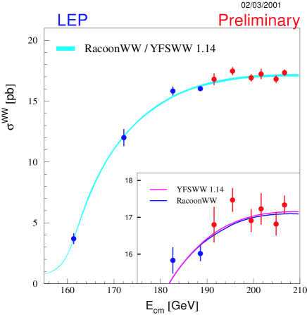
Figure 2: The CC03 production cross section vs. $\sqrt{s}$.

Figure 2 shows the measured $\mathrm{W}^{+}\mathrm{W}^{-}$ production cross section from threshold up to the highest collision energy reached at LEP2[5]. These data are compared with two recent theoretical calculations which include a more complete treatment of ${\cal O}(\alpha)$ radiative corrections through the double pole approximation[6, 7]. Good agreement is seen between the data and the newer calculations, which predict an overall rate (2.3–2.4)% lower than the older Gentle[8] semi-analytic calculation.

2.2 W-decay branching fractions at LEP2

Using the production rates observed in the ten unique $\mathrm{W}^{+}\mathrm{W}^{-}$ decay topologies, each LEP collaboration performs fits to its own data to extract the leptonic branching fractions individually, and with the additional constraint of lepton universality fits are performed for the hadronic branching fraction as well. In both cases, it is assumed that $\mathrm{Br}(\mbox{$\mathrm{W}\rightarrow\mathrm{q\overline{q}}$})+\mathrm{Br}(\mbox{$\mathrm{W}\rightarrow\ell{\nu_{\ell}}$})=1$. The combined LEP results are shown in Table 2[5].

Table 2: LEP combined W branching fractions.

Decay	Observed	SM Expectation
$\mathrm{Br}(\mbox{$\mathrm{W}\rightarrow\mathrm{e}\nu_{e}$})$	$10.54\pm 0.17$%	10.83%
$\mathrm{Br}(\mbox{$\mathrm{W}\rightarrow\mu\nu_{\mu}$})$	$10.54\pm 0.16$%	10.83%
$\mathrm{Br}(\mbox{$\mathrm{W}\rightarrow\tau\nu_{\tau}$})$	$11.09\pm 0.22$%	10.83%
$\mathrm{Br}(\mbox{$\mathrm{W}\rightarrow\mathrm{q\overline{q}}$})$	$67.92\pm 0.27$%	67.51%

The hadronic branching fraction can be interpreted as a measurement of the sum of the squares of the six elements of the CKM mixing matrix, $|\mathrm{V}_{ij}|$, which do not involve the top quark:

$${{\mathrm{Br}(\mbox{$\mathrm{W}\rightarrow\mathrm{q\overline{q}}$})}\over{1-\mathrm{Br}(\mbox{$\mathrm{W}\rightarrow\mathrm{q\overline{q}}$})}}=\left(1+\frac{\alpha_{s}(M_{\mathrm{W}})}{\pi}\right)\sum_{i={\mathrm{u,c}};\,j={\mathrm{d,s,b}}}\mbox{$|\mathrm{V}_{ij}|$}^{2}.$$ (1)

Taking $\alpha_{s}(M_{\mathrm{W}})$ to be $0.120\pm 0.005$, the branching fraction $\mathrm{Br}(\mbox{$\mathrm{W}\rightarrow\mathrm{q\overline{q}}$})$ from the combined LEP data yields

$$\sum_{i={\mathrm{u,c}};\,j={\mathrm{d,s,b}}}\mbox{$|\mathrm{V}_{ij}|$}^{2}=2.039\pm 0.025,$$ (2)

which is consistent with the value of 2 expected from unitarity in a three-generation CKM matrix.

Using the experimental knowledge of the sum, $\mbox{$|\mathrm{V}_{\mathrm{ud}}|$}^{2}+\mbox{$|\mathrm{V}_{\mathrm{us}}|$}^{2}+\mbox{$|\mathrm{V}_{\mathrm{ub}}|$}^{2}+\mbox{$|\mathrm{V}_{\mathrm{cd}}|$}^{2}+\mbox{$|\mathrm{V}_{\mathrm{cb}}|$}^{2}=1.048\pm 0.007$[9], the above result can be interpreted as a measure of $|\mathrm{V}_{\mathrm{cs}}|$ which is the least well determined of these matrix elements:

$$\mbox{$|\mathrm{V}_{\mathrm{cs}}|$}=0.996\pm 0.013.$$ (3)

A more direct determination of $|\mathrm{V}_{\mathrm{cs}}|$ is also performed by the LEP collaborations by counting the number of charm quarks produced in W events[10]. For example, Opal uses a multivariate analysis similar to what is used to tag b-quarks at LEP1 to extract a value of

$$R_{c}^{W}=0.481\pm 0.042\mathrm{(stat.)}\pm 0.032\mathrm{(syst.)}.$$ (4)

Using the relation

$$\Gamma(\mathrm{W}\rightarrow\mathrm{cX})=\frac{CG_{F}M_{\mathrm{W}}^{3}}{6\sqrt{2}\pi}(\mbox{$|\mathrm{V}_{\mathrm{cd}}|$}^{2}+\mbox{$|\mathrm{V}_{\mathrm{cs}}|$}^{2}+\mbox{$|\mathrm{V}_{\mathrm{cb}}|$}^{2}),$$ (5)

this measurement can again be interpreted in terms of $|\mathrm{V}_{\mathrm{cs}}|$, with fewer assumptions than the value shown in Equation 3:

$$\mbox{$|\mathrm{V}_{\mathrm{cs}}|$}=0.969\pm 0.058.$$ (6)

2.3 W boson production at the Tevatron

At the Tevatron, measurements are made of the production cross section times leptonic branching fraction for both W and Z bosons. These results from Run I are shown in Figure 3. Due to a different luminosity convention, the cross section quoted by CDF is 6% higher than that quoted by D0. The experimental uncertainties on these measurements are typically around 2% with a theoretical uncertainty of typically 3%, dominated by the knowledge of the parton distribution functions (PDFs). Since the luminosity uncertainty at the Tevatron is comparable, around 4%, at Run II it may well be advantageous to use the measurement of $\mathrm{Br}(\mbox{$\mathrm{W}\rightarrow\mathrm{e}\nu_{e}$})$ as a measure of the delivered luminosity.

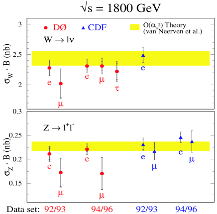
Figure 3: Tevatron production rates of W and Z bosons.

Using the ratio of electron production by W and Z bosons, the Tevatron collaborations perform a rather accurate indirect measurement of the W width. This ratio can be written as

$$\frac{\sigma\cdot\mathrm{Br}(\mbox{$\mathrm{W}\rightarrow\mathrm{e}\nu_{e}$})}{\sigma\cdot\mathrm{Br}(\mbox{$\mathrm{Z}\rightarrow ee$})}=\frac{\sigma_{\mathrm{W}}}{\sigma_{\mathrm{Z}}}\frac{\Gamma_{\mathrm{Z}}}{\Gamma(\mbox{$\mathrm{Z}\rightarrow ee$})}\frac{\Gamma(\mbox{$\mathrm{W}\rightarrow\mathrm{e}\nu_{e}$})}{\Gamma_{\mathrm{W}}},$$ (7)

where the ratio $\sigma_{\mathrm{W}}/\sigma_{\mathrm{Z}}$ is known from QCD[11], and the LEP1 measurement is used for $\mathrm{Br}(\mbox{$\mathrm{Z}\rightarrow ee$})$[12]. This can then be solved to extract the W branching fraction, which for CDF and D0 combined is

$$\mathrm{Br}(\mbox{$\mathrm{W}\rightarrow\mathrm{e}\nu_{e}$})=10.45\pm 0.20\,\%.$$ (8)

If it is additionally assumed that the electronic width of the W boson is equal to the Standard Model prediction $\Gamma(\mbox{$\mathrm{W}\rightarrow\mathrm{e}\nu_{e}$})=226.5\pm 0.3$ MeV[13], this can be interpreted as an indirect measurement of the total width,

$$\Gamma_{\mathrm{W}}(\mathrm{CDF+D0})=2.167\pm 0.040\,\mathrm{GeV},$$ (9)

in good agreement with the Standard Model prediction of $\Gamma_{\mathrm{W}}(\mathrm{SM})=2.093\pm 0.003$ GeV.

3 Electroweak Couplings

One of the fundamental predictions of the electroweak theory is the self-coupling of the gauge bosons due to the non-Abelian nature of the gauge fields. In general, there are seven unique couplings for each $WWV$ vertex which are Lorentz invariant, where $V$ denotes either of the neutral vector bosons. From an experimental point of view, this represents far too many individual parameters to measure, and several assumptions and constraints have been applied to reduce this to a more manageable set of three. First, considerations of gauge invariance, $C$, $P$, and $CP$ conservation are used to reduce this set down to five, which are usually denoted as $\kappa_{\gamma},\kappa_{\mathrm{Z}},\lambda_{\gamma},\lambda_{\mathrm{Z}},g_{1}^{\mathrm{Z}}$. The Standard Model predicts that only three of these couplings are non-zero, with $\kappa_{\gamma}=\kappa_{\mathrm{Z}}=g_{1}^{\mathrm{Z}}=1$. More familiar static properties of the W boson are then some function of the general couplings, for example the magnetic dipole moment is given as $\mu_{\mathrm{W}}=e(1+\kappa_{\gamma}+\lambda_{\gamma})/2M_{\mathrm{W}}$.

The precision electroweak data collected at LEP1 and the SLC can be used to further constrain the allowed couplings down to a set of three. This precision data implies the relations $\Delta\kappa_{\mathrm{Z}}=-\Delta\kappa_{\gamma}\tan^{2}\!\theta_{\mathrm{W}}+\Delta g_{1}^{\mathrm{Z}}$ and $\lambda_{\gamma}=\lambda_{\mathrm{Z}}$, where $\Delta\kappa_{\mathrm{Z}}=\kappa_{\mathrm{Z}}-1$ is the deviation from the Standard Model prediction.

3.1 Triple gauge couplings at LEP2

Figure 4: LEP2 processes sensitive to triple gauge couplings.

At LEP2, triple gauge coupling (TGC) analyses consider the processes shown in Figure 4. Most of the sensitivity arises from W-pair production, although the single-W diagram and single photon production help constrain $\kappa_{\gamma}$ which is otherwise poorly measured in high energy $\mathrm{e}^{+}\mathrm{e}^{-}$ collisions. The presence of anomalous TGCs will modify both the total cross section and the differential cross sections of these processes, and the LEP analyses make use of all of this information to extract TGC limits.

LEP combined limits are obtained for both single-parameter fits with the other two anomalous couplings fixed to zero, and for multi-dimensional fits where two or all three anomalous couplings are allowed to deviate from zero. The most recent results for the LEP single parameter fits are

$$\Delta\kappa_{\gamma} = -0.002\pm 0.066$$

$$\Delta g_{1}^{\mathrm{Z}} = -0.025\pm 0.026$$ (10)

$$\lambda_{\gamma} = -0.036\pm 0.028$$

where the errors indicate the one sigma (68% CL) errors of the fit. Examples of multi-dimensional confidence level regions are shown in Figure 5. These results date from ICHEP 2000[14] and do not include potentially large corrections arising from ${\cal O}(\alpha)$ radiative corrections which have recently been included into standard Monte Carlo generators. New combined results taking these effects into account should be available by the Summer conferences of 2001. At any rate, the precision of these measurements is at the 3% level for all but $\Delta\kappa_{\gamma}$, which is the most difficult coupling to measure at LEP2.

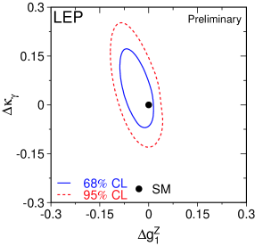
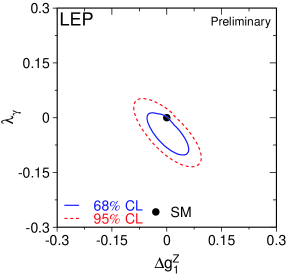
Figure 5: LEP2 combined two-dimensional TGC fits.

3.2 Triple gauge couplings at the Tevatron

The Tevatron collaborations can also measure triple gauge couplings through either associated production of the W boson accompanied by a neutral gauge boson, or through direct W-pair production. The most useful final state for associated production is $\ell{\nu_{\ell}}+\gamma$, where a real photon is radiated directly from the W. Equivalent diagrams involving a Z boson are marginal at Run I, but should become useful at Run II. In the case of W-pair production, the $\ell\nu\ell\nu$ and $\mathrm{qq}\ell\nu$ final states are analyzed. Similarly to LEP, the sensitivity to TGCs at the Tevatron arise from both an increase in the total rate for these processes, but also from the shape of the various differential cross sections. D0, for example, performs a combined analysis to the $\ell{\nu_{\ell}}+\gamma$, $\ell\nu\ell\nu$, and $\mathrm{qq}\ell\nu$ channels using both the overall rate and the $p_{\mathrm{T}}^{\,\mathrm{W}}$ distributions as fit variables.

Fitting for two TGC parameters, D0 obtains the following 95% confidence level limits

$$\begin{array}[]{rcccl}-0.25&\leq&\Delta\kappa&\leq&+0.31\\ -0.18&\leq&\lambda&\leq&+0.18\end{array}$$ (11)

where in each case the second coupling is fixed to be zero[15]. With the increased luminosity and collision energy expected at Run II, these results should improve by a factor of two to three, which will make D0 competitive with any single LEP experiment.

3.3 Quartic gauge couplings

Figure 6: LEP2 processes sensitive to anomalous quartic gauge couplings.

The Standard Model also predicts a genuine four-point interaction involving only gauge bosons. Some of the LEP collaborations have performed analyses using the diagrams shown in Figure 6 to attempt to observe these quartic gauge couplings (QGCs). Since the predicted strength of this coupling in the Standard Model is negligible at LEP2, any deviation from zero would be evidence for anomalous QGCs.

The Lorentz structure of the four-boson vertex can be parameterized in a manner similar to that used in the TGC case. The LEP collaborations have explored the possibility of two $CP$-conserving parameters $a_{0}$ and $a_{c}$ which involve the $\mathrm{WW}\gamma\gamma$ vertex[16], along with a single $CP$-violating coupling $a_{n}$ which involves the $\mathrm{WWZ}\gamma$ vertex[17]. In addition, analyses have been performed for QGCs involving purely neutral gauge bosons.

In the $\mathrm{WW}\gamma$ final state, the signature of anomalous QGCs is an enhancement of the hard photon spectrum above that expected from other radiative processes. An example of this spectrum from L3 is shown in Figure 7.

Figure 7: L3 photon spectrum for $\mathrm{WW}\gamma$ QGC analysis.

An unofficial LEP combination of the available QGC results from Aleph, Opal, and L3 was presented at Moriond 2001[18]. The combined limits at the 95% CL in units of $\mathrm{GeV}^{2}$ are

$$\begin{array}[]{rcccl}-0.022&\leq&a_{0}/\Lambda^{2}&\leq&+0.021\\ -0.043&\leq&a_{c}/\Lambda^{2}&\leq&+0.058\\ -0.22&\leq&a_{n}/\Lambda^{2}&\leq&+0.20.\end{array}$$ (12)

4 W Mass and Width

When combined with other precision electroweak data, most notably the mass of the Z boson, the W boson mass becomes a fundamental prediction of the Standard Model. Testing this prediction with ever increasing precision has been a goal of particle physics over the last decade, both to verify the Standard Model, but also to gain insight into what may lie beyond. In this section, the measurements of $M_{\mathrm{W}}$ at the Tevatron and LEP2 are described.

4.1 W mass at the Tevatron

Figure 8: W boson production in $\mathrm{p}\bar{\mathrm{p}}$ collisions.

It is customary to think of W production at the Tevatron in terms of the simple process $\mathrm{q\overline{q}}\rightarrow\mathrm{W}\rightarrow\ell{\nu_{\ell}}$, while in reality the actual event is considerably more messy. As shown in Figure 8, along with the W boson comes hard gluon radiation which must balance the W boson $p_{\mathrm{T}}$, along with the ever-present spectator and multiple interaction background from the $\mathrm{p}\bar{\mathrm{p}}$ collision.

Since there is essentially no information available regarding the longitudinal boost of the W boson, CDF and D0 both use the transverse mass as the fundamental observable in their W mass analysis. The transverse mass is given by

$$m_{\mathrm{T}}=\sqrt{2E_{\mathrm{T}}^{\,\ell}E_{\mathrm{T}}^{\,\nu}(1-\cos\phi_{\ell\nu})},$$ (13)

where the neutrino is defined in terms of the missing transverse momentum $\vec{p}_{\mathrm{T}}^{\,\nu}=-(\vec{p}_{\mathrm{T}}^{\,\ell}+\vec{U})$ with $\vec{U}$ representing the transverse momentum of the hard QCD recoil.

In general terms, the mass analysis at the Tevatron involves fitting the transverse mass spectrum observed in the data with a Monte Carlo prediction of this spectrum which depends upon $M_{\mathrm{W}}$. An example of such a fit from CDF is shown in Figure 9. There are a number of individual components necessary to construct the model of the $m_{\mathrm{T}}$ spectrum, each of which contributes to the overall systematic error of the measurement. The three most important are described below.

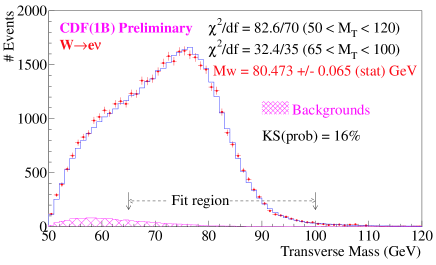
Figure 9: CDF transverse mass spectrum for $\mathrm{W}\rightarrow\mathrm{e}\nu_{e}$.

Firstly, the energy scale and resolution of the detector to leptons and hadrons must be precisely modelled. This modelling can be constrained using control samples found in the data, most notably ${\mathrm{Z}^{0}}\rightarrow\ell^{+}\ell^{-}$ decays which have a very similar topology to the W decays of interest. D0, for example, calibrates their detector response to electrons by fitting to the observed invariant mass distributions for $\pi^{0}\rightarrow eeee$, $\mathrm{J}/\Psi\rightarrow ee$, and ${\mathrm{Z}^{0}}\rightarrow ee$. The uncertainty on the detector response is largely driven by the statistics available in the available control samples, and will improve considerably in Run II. A list of typical uncertainties is shown in Table 3[19].

Table 3: Typical Tevatron W mass uncertainties per channel. An indication is also given whether an uncertainty is largely statistical or correlated between CDF and D0.

Source	Uncertainty (MeV)	Statistical?	Correlated?
statistical	60 - 100	yes
scale	80	yes
resolution	25	yes
backgrounds	15
recoil	40	yes
PDFs	15	yes	yes
higher orders	15		yes

Secondly, the transverse momentum spectrum of the QCD recoil must be modelled properly. Again, control samples in the data provide powerful constraints to tune the production models used in the Monte Carlo generators. By comparing the transverse momentum observed in ${\mathrm{Z}^{0}}\rightarrow\ell^{+}\ell^{-}$ events, where there is no missing neutrino, adequate statistics can be found to limit this uncertainty to an acceptable level.

Finally, the parton density functions (PDFs) used to describe the constituents of the incoming $\mathrm{p}\bar{\mathrm{p}}$ system must be constructed. Knowledge of these PDFs comes from a wide variety of data made at the Tevatron and elsewhere[20]. Although this is currently a rather modest uncertainty at the level of 15 MeV, since it is correlated between both experiments and rather difficult to constrain directly with Tevatron data, it could become a limiting systematic at Run II.

While the general analysis strategy for the W mass is similar between CDF and D0, there are significant differences in the details. CDF analyzes $\mathrm{W}\rightarrow\mathrm{e}\nu_{e}$ and $\mathrm{W}\rightarrow\mu\nu_{\mu}$ events where the lepton is reconstructed in the central detector region $(|\eta_{\ell}|<1)$. D0 uses only $\mathrm{W}\rightarrow\mathrm{e}\nu_{e}$, although electrons in the forward detector region are also included $(1.5<|\eta_{\ell}|<2.5)$. In addition, D0 performs a fit not only to the transverse mass spectrum, but also to the transverse momentum spectra $p_{\mathrm{T}}^{\,e}$ and $p_{\mathrm{T}}^{\,\nu}$.

The final W mass results from the Tevatron collaborations for Run I are

$$\begin{array}[]{lccl}M_{\mathrm{W}}(\mathrm{CDF})&=&80.433\pm 0.079&\mathrm{GeV}\\ M_{\mathrm{W}}(\mathrm{D0})&=&80.482\pm 0.091&\mathrm{GeV},\end{array}$$ (14)

which when combined accounting for correlated systematic uncertainties yields a W mass measurement of[21]

$$M_{\mathrm{W}}(\mathrm{p}\bar{\mathrm{p}})=80.452\pm 0.062\,\mathrm{GeV}.$$ (15)

It should be noted that D0 is updating their ‘final’ Run I result in Summer 2001 by adding additional $\mathrm{W}\rightarrow\mathrm{e}\nu_{e}$ events where the electrons went into detector regions previously considered unusable. With this additional data, the combined D0 results should be quite competitive with the final CDF Run I measurement.

The prospects for the W mass measurement are quite encouraging. With 2 $\mathrm{fb}^{-1}$ expected in Run IIa, there is significant room for improvement both in the statistical and systematic uncertainties, since many of these systematics are limited by available control samples. It is expected that a total uncertainty of under 40 MeV per experiment can be achieved in Run IIa.

4.2 W mass at LEP2

While the sample of W bosons collected at LEP2 is significantly smaller that that collected at the Tevatron, the benefits of a clean $\mathrm{e}^{+}\mathrm{e}^{-}$ collision environment allow more information to be extracted from each event recorded. In particular, the well defined initial state allows the use of constrained kinematic fitting to greatly improve the mass resolution on the reconstructed W boson. All four LEP collaborations measure the W mass by a method of direct reconstruction based on constrained kinematic fitting, although the exact details of each analysis can vary significantly.

Four constraints are imposed on the kinematics of each event requiring that the initial $\mathrm{e}^{+}\mathrm{e}^{-}$ system is at rest in the center of mass and has an energy equal to twice the incoming beam energy. In some analyses, an additional fifth constraint forcing the two W boson masses to be equal, is also imposed. For the semi-leptonic $\mathrm{qq}\ell\nu$ final states, there is a single neutrino which is not measured, leaving a two constraint fit after the equal mass constraint is applied. For the fully hadronic $\mathrm{qqqq}$ final states, there is no missing momentum and a full four or five constraint fit is possible depending upon whether the equal mass constraint is used.

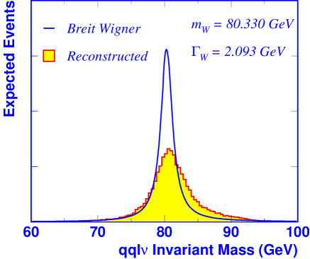
Figure 10: Reconstructed $\mathrm{qq}\ell\nu$ invariant mass spectrum from Monte Carlo.

The reconstructed mass spectrum, as shown for example in Figure 10, looks rather different than a pure relativistic Breit–Wigner distribution for several reasons. Firstly, the presence of initial state radiation (ISR) means that the actual energy producing the W pairs is always less than twice the incoming beam energy. This tends to cause a tail towards higher invariant masses, as the collision energy assumed in the kinematic fit is overestimated. Secondly, effects of detector resolution tend to significantly smear out the lineshape as the experimental resolution is not significantly better than the W boson width for most channels. Finally, the effects of non-CC03 diagrams, particularly in the $\mathrm{q\overline{q}}\mathrm{e}\nu_{e}$ channel, distort the lineshape due to the interference with the resonant production amplitudes.

As a result, the W boson mass can not be extracted by simply fitting an analytic Breit–Wigner shape, but rather must rely on a Monte Carlo simulation of these various effects to model the dependence of the spectrum on $M_{\mathrm{W}}$. Delphi uses a likelihood convolution technique to construct a likelihood $\cal{L}(M_{\mathrm{W}})$ for each event. The remaining three collaborations currently use re-weighting techniques to construct Monte Carlo templates at arbitrary $M_{\mathrm{W}}$ to be fit to the data distributions.

The fully hadronic $\mathrm{qqqq}$ final state has the additional complication of a three-fold ambiguity in pairing the observed jets to the underlying W bosons. Aleph and Opal use an additional jet pairing algorithm to choose for each event which pairing is most likely to be correct. L3 uses the single pairing which yields the highest kinematic fit probability, while Delphi can naturally use all three combinations appropriately weighted in the likelihood convolution technique.

Figure 11 shows some mass spectra compared to the Monte Carlo fits for Aleph data recorded during the final year of LEP running.

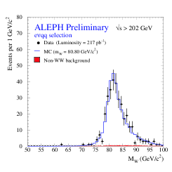
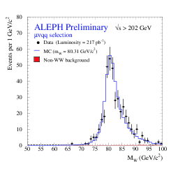
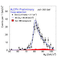
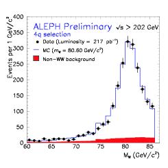
Figure 11: Reconstructed mass spectra from the Aleph collaboration.

The four LEP collaborations combine their results taking into account systematic uncertainties which are correlated between channels, experiments, and years of LEP running. This combination procedure is still evolving, as better information about the nature of these various correlations becomes available. The preliminary combined LEP W mass result from direct reconstruction presented at Moriond 2001 is

$$M_{\mathrm{W}}(\mathrm{LEP})=80.447\pm 0.026\mathrm{(stat.)}\pm 0.030\mathrm{(syst.)}\,\mathrm{GeV},$$ (16)

where the component of the total uncertainty coming from statistical and systematic sources is indicated[22]. As can be seen in the detailed breakdown of these uncertainties shown in Table 4, the $\mathrm{qqqq}$ channel has rather large uncertainties associated with Bose–Einstein correlations and color reconnection. Due to these uncertainties, the $\mathrm{qqqq}$ channel carries a weight of only 27% in the combined result, even though it is statistically more precise. If there were no sources of systematic uncertainty, the combined statistical error would be 22 MeV.

Table 4: Uncertainties on the LEP combined W mass.

Uncertainty	$\mathrm{qq}\ell\nu$ (MeV)	$\mathrm{qqqq}$ (MeV)	Combined (MeV)
ISR/FSR	8	8	7
Hadronization	19	17	18
Detector	11	8	10
Beam Energy	17	17	17
Color Recon.	-	40	11
Bose-Einstein	-	25	7
Other	4	5	3
Total Syst.	29	54	30
Statistical	33	31	26
Total	44	62	40

The most important uncertainties for the LEP W mass measurement are related to the modelling of the detector response, modelling the hadronization of quarks into jets, understanding the LEP beam energy, and the final state interactions mentioned before. To limit the uncertainty from detector modelling, the LEP collider was run from time to time throughout each running year at the ${\mathrm{Z}^{0}}$ resonance to take large samples of ${\mathrm{Z}^{0}}\rightarrow\ell^{+}\ell^{-}$ and ${\mathrm{Z}^{0}}\rightarrow\mathrm{q\overline{q}}$events. These samples, as well as similar samples at high energy, are then used to study the detector response to leptons and jets and limit the deficiencies in the detector models. Hadronization uncertainties are estimated by comparing different Monte Carlo implementations of the hadronization process, including Jetset[23], Herwig[24], and Ariadne[25]. Knowledge of the LEP beam energy is critically important as it sets the overall energy scale for the W mass measurement, and any uncertainty in is completely correlated between all four LEP collaborations. More detailed information about the beam energy measurement at LEP2 can be found elsewhere[26].

The broad issue of final state interactions (FSI) involves any effect in the $\mathrm{qqqq}$ channel by which the decay products of the two W bosons interact with each other. Since standard Monte Carlo models assume that these two systems decay independently, these interactions can exchange momentum between the two W systems and distort the final W lineshape. Two specific phenomena which are known to exist, but with rather uncertain strengths, are color reconnection (CR) and Bose–Einstein correlations (BEC).

Color reconnection involves the rearrangement of the color strings in the hadronizing system, essentially gluon exchange, in the non-perturbative phase of the hadronization process. Only a few models exist to describe this process, and these tend to have limited predictive power[27]. Bose–Einstein correlations between identical particles are well established in hadronic ${\mathrm{Z}^{0}}$ decays at LEP1. Since the W boson decay length (0.1 fm) is significantly shorter than the hadronization scale (1 fm), it is entirely plausible that there can be additional BE effects between particles originating from different W bosons in $\mathrm{qqqq}$ events. Because of the way Monte Carlo generators operate, however, modelling this purely quantum mechanical effect is extremely difficult, and imperfect knowledge of the space-time evolution of the hadronizing system adds to the difficulty[28].

Overall, the strategy of the LEP experiments to address these difficult questions is to use the various models as a guide for the types of effects which can be expected, but to constrain the allowed magnitude of any FSI effect using the data directly. One way to broadly check that large FSI effects are not present is to compare the W mass measured in the $\mathrm{qqqq}$ channel to that measured in the $\mathrm{qq}\ell\nu$ channel. Including all uncertainties with their correlations aside from those related to FSI directly, the LEP collaborations find

$$M_{\mathrm{W}}(\mathrm{qqqq})-M_{\mathrm{W}}(\mathrm{qq}\ell\nu)=+18\pm 46\,\mathrm{MeV},$$ (17)

which is consistent with no final state interactions.

Color reconnection effects tend to enhance or suppress particle production in the regions between the main jets. Currently, all four LEP collaborations are pursuing analyses aimed at measuring the particle flow distribution in $\mathrm{qqqq}$ final states with the ultimate aim of discriminating between various CR models. With all four LEP experiments combined, it is likely that the uncertainty from CR can be significantly reduced from its current values.

The analysis of BEC effects is in a more advanced stage. All four LEP collaborations are currently using an event mixing method where data from two semi-leptonic $\mathrm{qq}\ell\nu$ events are mixed (without the lepton) and compared to data from genuine $\mathrm{qqqq}$ events. In a rigorously model–independent test, these two samples should look identical if there is no BEC present between the decay products of different W bosons. In order to limit the possible size of the effect allowed, however, a similar analysis must be performed on different Monte Carlo models of BEC. Currently, all four LEP collaborations see no evidence for inter-W BEC effects at the limits of their statistical power to observe them. By combining these results and evaluating a range of BEC models, the systematic uncertainty from this source should also be reduced for the final LEP results.

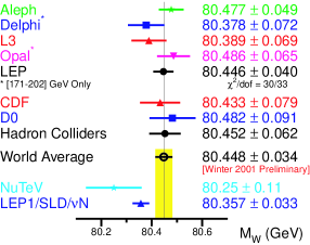
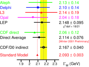
Figure 12: World results on the mass and width of the W boson.

The current world knowledge of the W mass from LEP2 and the Tevatron are shown in Figure 12, along with the indirect value inferred from other precision electroweak measurements. While the current world average is dominated by LEP2, with the data expected at the Tevatron during Run IIa, the combined error on direct W mass measurements should approach 20 MeV by around 2006.

4.3 W width measurements

The direct reconstruction method employed at LEP2, as well as the transverse mass method employed at the Tevatron, are sensitive to the W width as well as the W mass. In the standard mass analyses, the width is typically fixed to the Standard Model expectation for a given mass value, but it can equally well be allowed to be a second free parameter in the fits. The direct measurements of the W boson width are shown in Figure 12 along with the indirect width evaluation mentioned earlier and the Standard Model expectation. It should be noted that not all LEP data has been analyzed, and D0 has yet to produce a result for the direct width measurement. With these improvements, the precision on the direct width measurements should actually be competitive with the indirect width from the Tevatron.

5 Conclusions

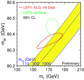
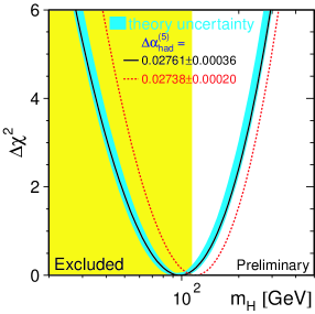
Figure 13: World combined electroweak results.

The combined electroweak data is often summarized as shown in Figure 13. The first plot in this figure shows $M_{\mathrm{W}}$ vs. $M_{\mathrm{t}}$ both for the direct measurements, the indirect electroweak data, and the Standard Model prediction as a function of the Higgs mass. It is clear that a light Higgs is preferred by the data, and the direct measurements are starting to stray into a region more favorable for Supersymmetric theories. It can also be seen from this plot that significant improvements in the uncertainty on $M_{\mathrm{W}}$ will not be very useful if they are not accompanied by comparable improvements in $M_{\mathrm{t}}$.

Another way of looking at this is in terms of the sensitivity toward the remaining unknown parameter in the Standard Model, the Higgs mass. Several groups have produced simple parameterized versions of the functional relationships predicted by the Standard Model between derived quantities like $M_{\mathrm{W}}$ or $\sin^{2}\!\theta_{\mathrm{W}}$ and the input parameters like $M_{\mathrm{t}}$ and $M_{\mathrm{H}}$[29]. Using these tools, it can be shown that after Run IIa, the constraint on the Higgs mass arising from the measurement of the W mass is improved in equal parts by reducing the uncertainty on $M_{\mathrm{W}}$, but also by reducing the uncertainty on $M_{\mathrm{t}}$which is necessary to calculate the Standard Model prediction. It can also be seen that the constraint arising from the W mass will match the precision of that coming from $\sin^{2}\!\theta_{\mathrm{W}}$, and with greatly reduced sensitivity to the running of the fine structure constant[30].

In summary, the past five years have seen some remarkable improvements in the knowledge of the W boson properties from the LEP collaborations. With around 650 $\mathrm{pb}^{-1}$ recorded per experiment, world’s best measurements of the W boson branching fractions, gauge couplings, and mass have been performed. The next five years will see measurements of similar precision performed at the Tevatron with the advent of Run II. The combined electroweak data continues to provide the most stringent constraint for any model of new physics, and improving this knowledge is crucial step to the eventual goal of fully understanding the process of electroweak symmetry breaking.

6 Acknowledgements

The author would like to thank the organizers for the kind invitation to participate in this conference, as well as a warm personal thanks to the local organizing committee for their efforts to make this event pleasant for everybody. The author would also like to thank the members of the Aleph, Delphi, L3, Opal, CDF, and D0 collaborations for their assistance in preparing this paper.

References

- 1 . Proceedings of CERN LEP2 Workshop, CERN 96-01, Vols. 1 and 2, eds. G. Altarelli, T. Sjöstrand and F. Zwirner.
-
2 .
S. Jadach et al., Comp. Phys. Comm. 119 272 (1999);
M. Skrzypek et al., Comp. Phys. Comm. 94 216 (1996);
M. Skrzypek et al., Phys. Lett. B372 289 (1996). - 3 . F.A. Berends, R. Pittau and R. Kleiss, Comp. Phys. Comm. 85 437 (1995).
- 4 . J. Fujimoto et al., Comp. Phys. Comm. 100 128 (1997).
- 5 . The LEP Collaborations and the LEPEW Working Group, LEPEWWG/XSEC/2001-01.
-
6 .
S. Jadach, et al.,
“Precision Predictions for (Un)Stable Pair Production at and
Beyond LEP2 Energies,”
UTHEP-00-0101, hep-ph/0007012, Submitted to Phys. Lett. B;
S. Jadach, et al., Phys. Rev. D61 113010 (2000). - 7 . A. Denner, S. Dittmaier, M. Roth and D. Wackeroth, Nucl. Phys. B 587, 67 (2000).
- 8 . D. Bardin et al., Comp. Phys. Comm. 104 161 (1997).
- 9 . Particle Data Group, D.E. Groom et al., Eur. Phys. J. C15 1 (2000).
-
10 .
G. Abbiendi et al. [OPAL Collaboration],
Phys. Lett. B 490, 71 (2000);
R. Barate et al. [ALEPH Collaboration], Phys. Lett. B 465, 349 (1999). - 11 . R. Hamberg, W. L. van Neerven and T. Matsuura, Nucl. Phys. B 359, 343 (1991).
- 12 . The LEP Collaborations and the LEP EW Working Group, CERN-EP-2000-153, to appear in Phys. Rep..
- 13 . J. L. Rosner, M. P. Worah and T. Takeuchi, Phys. Rev. D 49, 1363 (1994).
- 14 . The LEP Collaborations and the LEPEW Working Group, LEPEWWG/TGC/2000-02.
- 15 . B. Abbott et al. [D0 Collaboration], Phys. Rev. D 62, 052005 (2000).
- 16 . G. Belanger and F. Boudjema, Phys. Lett. B 288, 210 (1992).
- 17 . W. J. Stirling and A. Werthenbach, Eur. Phys. J. C 12, 441 (2000).
- 18 . M. Musy, XXXVIth Rencontres de Moriond on Electroweak Interactions (2001) hep-ex/0105063.
- 19 . D. Glenzinski, XXXVIth Rencontres de Moriond on Electroweak Interactions (2001).
-
20 .
M. Glück et al., Z. Phys. C67, 433 (1995);
H.L. Lai et al., Phys. Rev. D51, 4763 (1995);
A.D. Martin et al., Phys. Rev. D50, 6734 (1994). -
21 .
T. Affolder et al. [CDF Collaboration],
Phys. Rev. D 64, 052001 (2001);
B. Abbott et al. [D0 Collaboration], Phys. Rev. Lett. 84, 222 (2000). - 22 . The LEP Collaborations and the LEPEW Working Group, LEPEWWG/MASS/2001-01.
- 23 . T. Sjöstrand, Comp. Phys. Comm. 82 74 (1994).
- 24 . G. Marchesini et al., Comp. Phys. Comm. 67 465 (1992).
- 25 . L. Lonnblad, Comput. Phys. Commun. 71, 15 (1992).
- 26 . LEP Energy Working Group, A. Blondel, et al., Eur. Phys. J. C11 573 (1999).
-
27 .
T. Sjöstrand and V.A. Khoze, Z. Phys. C62 281 (1994);
Phys. Rev. Lett. 72 28 (1994);
L. Lönnblad, Z. Phys. C70 107 (1996). - 28 . L. Lönnblad and T. Sjöstrand, Eur. Phys. J. C2 165 (1998).
-
29 .
G. Degrassi and P. Gambino, Nucl. Phys. B 567, 3 (2000);
A. Freitas, W. Hollik, W. Walter and G. Weiglein, Phys. Lett. B 495, 338 (2000). - 30 . E. Tournefier, XXXVIth Rencontres de Moriond on Electroweak Interactions (2001) hep-ex/0105091.