A device to characterize optical fibres

Abstract

ATLAS is a general purpose experiment approved for the LHC collider at CERN. An important component of the detector is the central hadronic calorimeter; for its construction more than 600,000 Wave Length Shifting (WLS) fibres (corresponding to a total length of 1,120 Km) have been used. We have built and put into operation a dedicated instrument for the measurement of light yield and attenuation length over groups of 20 fibres at a time. The overall accuracy achieved in the measurement of light yield (attenuation length) is 1.5% (3%). We also report the results obtained using this method in the quality control of a large sample of fibres.

,

1 Introduction

Optical fibres have been widely used in recent years in High Energy Physics. Their popularity is due to several factors: cost; efficiency in light transport; easiness to machine and adapt to various geometries. Both scintillating fibres and WLS fibres have found many applications in HEP detectors, in the field of tracking: UA2 [1], $D\emptyset$ [2], as active elements in calorimeters: KLOE(DA$\Phi$NE) [3], CHORUS [4], H1(DESY) [5], and as efficient devices to transport light from scintillators to the photomultipliers: ZEUS(HERA) (presampler calorimeter) [6], DELPHI(LEP)(stic detector) [7].

The device presented in this paper was developed during the construction of the hadron calorimeter (Tile Calorimeter) of ATLAS [8], one of the two major detectors that will acquire data in the forthcoming years at LHC.

The Tile Calorimeter [9] is an iron-scintillator calorimeter whose geometry has been designed to minimize dead spaces and optimize hermeticity. The two main characteristics are: the orientation of the scintillator tiles along the direction of the incoming particles, and the use of WLS fibres to transport light to photomultipliers (PMTs). The ensemble of these two choices allowed an extremely compact design of the calorimeter with virtually no dead spaces.

The constraints imposed by this design on the performance of fibres, are severe, as we will discuss in the following section. The quality of the fibres had to be carefully monitored all along the production period. The fibres were produced in batches and the control of quality (QC), had to be precise and fast enough to detect and correct in real time possible deviations from the optimal requirements of the fibre characteristics.

2 Requirements on the fibres

The optical contact of scintillating tiles with WLS fibres is obtained by gently pressing the fibres for a fraction of their length against the side of the scintillators. A diffuser surrounds the fibre and the scintillator, increasing the light collection efficiency. Only a small fraction of light is captured by the fibres, as the wavelength shifting efficiency and the effective light attenuation length in the fibre, reduce considerably the number of photons which reach the PMT. The overall light budget is about 40-60 photoelectrons (phe) per GeV deposited in a calorimeter cell. To obtain a higher light yield, we decided to use double-clad fibres which, with respect to single clad fibres, ensure a larger capture efficiency of light rays and longer attenuation length. Severe requirements were placed on the wavelength shifting efficiency and on the effective attenuation length of light in the fibre. Conventionally we characterize the fibres by two quantities:

1. the attenuation length ($\lambda$), that is obtained by measuring the light yield at one end, after exciting the fibre at several positions along its length;

2. the light yield ($n_{0}$) obtained by exciting the fibre at 140 cm from the end.

The QC requires these two quantities to be as large as possible and at the same time the spread among individual measurements to be as small as possible. In fact any large fluctuations of these quantities would produce dis-homogeneities in the calorimeter response, resulting in non-statistical terms in the calorimeter resolution (the so called “constant terms”).

The limits on these parameters and on fluctuations in their values have been assesed using careful MonteCarlo simulations requiring that the calorimeter resolution would not be significantly affected by fibre performance even in the long run, when we expect small aging effects to show up.

3 The fibrometer

The total length of fibres needed for the Tile Calorimeteris 1,120 Km, a quantity which can be produced by a commercial firm in about one year. The length of individual fibres ranges from 73 to 230 cm and the total number of fibres is about 640,000. It was not possible to measure all the fibres, neither was it appropriate, since during the measurement process the fibres might undergo damage.

Each batch of fibres was composed of about 30 production units called “preforms”. Because of the production process, the fibres within a preform are quite uniform. Preforms could slight differ from each other, because of different chemical composition, temperature, tension in pulling fibres, etc. One preform consist of about 2,000 fibres.

We decided to measure 18 fibres of each preform, randomly chosen. This number allows a precise enough determination of the mean and R.M.S. of the whole preform. Still, more than 3,000 fibres had to be measured. An instrument to perform a rapid and precise measurement was therefore designed. We developed a dedicated apparatus which allows a fast and precise characterization of 20 fibres in parallel.

The main idea is to hold the fibres under measurement on a precision plate which is fixed to an optical test bench. The fibres are excited by a movable light source that can be positioned with an x-y table over the fibre plate. The fibres are read by a single PMT, connected to the fibres under measurement through clear fibres. Hence the only movable part of the system is the light source.

The light source is a blue LED. Great care is given to the stability of the light source and to the gain of the PMT. Both are monitored electronically; but the stability of the system is finally checked by comparison with two reference fibres which have been mounted on the plate at the beginning of the measurements and never moved.

3.1 Construction Details

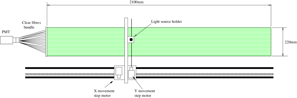
Figure 1: General view of the setup for fibre characterization.

A sketch of the fibrometer is shown in Fig. 1. The aluminum plate which holds in place the fibres is 2 m long and is installed on a granite optical table. The aluminum plate was machined to obtain 20 parallel V-shaped grooves that house the fibres under measurement. The distance between adjacent grooves is 1 cm, each groove being 0.65 mm deep with an angle of 90 degrees. Details of the grooves geometry are shown in Fig. 2 (a) which shows a cross section of the plate. A 4 mm high wall between the grooves reduces any possible cross-talk between nearby fibres. The plate is black anodized to avoid spurious reflections. Fibres are kept fixed to the plate at three positions: in the middle and at the two ends. At these points the shape of the grooves is appropriately modified in such a way that the fibres can be hold in place by the preassure applied through the use of small soft-rubber pieces. Table and fibrometer are placed inside a light-tight dark room.

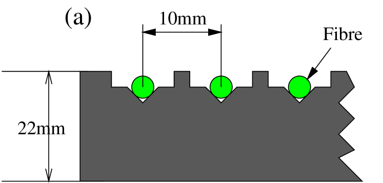
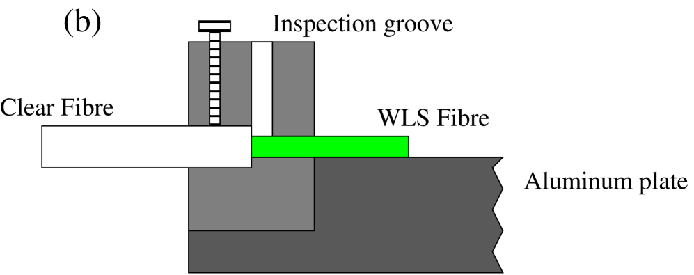
Figure 2: Side view of fibre plate (a) and detail of coupling between clear and WLS fibres (b).

The fibres are excited using a light source with an emission spectrum similar to the one of the Tile Calorimeter plastic scintillators. The absolute response of fibres to this light source is not identical to the scintillation light, since the spectral emission is not exactly the same. This, however, does not affect the results of the QC. As a light source we have used a very intense blue LED ($\bar{\lambda}$=430 nm) DC operated. The LED was mounted on a x-y table movable in precise steps (3 mm along and 5 $\mu$m across the fibres, for each clock pulse). The LED was kept within a PVC case at about 20 cm from the fibres. The light is collimated with a 0.7 mm slit, placed at 5 mm from the fibres. The size of the light spot was 0.8 mm at the fibre. Cross-talk effects between fibres were, under these conditions, negligible.

The LED source is clearly much easier and safer to handle than a light source made of a plastic scintillator and a radioactive source. The latter is much more stable and would reproduce exactly the light spectrum of the detector. The LED on the contrary has to be calibrated with respect to the scintillator light and continuously monitored in intensity. After having considered the pros and cons of the two solutions the LED system was finally chosen.

Fig. 1 shows some details of the x-y table used for the positioning of the light source. Two rails, mounted rigidly on an optical bench, and a precise gear allow the movement of a motorized head along the fibres (x-direction). The head supports a light aluminum arm, orthogonal to the rails, on which the light source is mounted. Precision rails guide the movement across the fibres (y-direction) of the light source. Both movements are driven by step motors under computer control. No sensor was used to monitor the position of the light source, which is obtained by counting the number of steps of the motors. This implies that any clock pulse lost in the motor driving electronics would result in a wrong positioning of the light source. From the following discussion it will be clear that the system is self-calibrating in position across the fibres where the measurement steps are very fine (0.1 mm). A large step size (10 cm), between consecutive measurements, was chosen for the movement along the fibres. Therefore the loss of one or a few clock pulses would be unimportant.

Twenty, 2 mm diameter, clear fibres provide the light collection. One end of the clear fibre is optically machined, mounted on the fibre plate and held in position by a teflon screw (Fig. 2 b). The fibres under measurement are optically coupled to the clear ones by air coupling. The other ends of the clear fibres are glued together inside a Plexiglas tube and optically machined. The clear fibre bundle faces a PMT through a light mixer. A single PMT receives the light of all the twenty fibres which are excited one at a time. The signals from the PMT are sampled every 30 ms by a digital multi-meter. Fig. 3 shows the granite table with the fibrometer mounted on it.

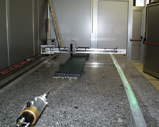
Figure 3: Photograph of the setup for fibre characterization.

The Data Acquisition System controls the operation of the stepping motors and performs the synchronous readout of the multi-meter. It is based on a FIC OS9 housed in a VME crate. The I/O electronics is CAMAC based, a VME-CAMAC interface provides the interconnections between the two systems. Fig. 4 shows a schematics of the readout electronics.

Figure 4: Schematics of the readout electronics.

An important point in the construction of the fibrometer is the stability in parallelism between the plate that holds the fibres and the light source. Any deviation from parallelism during the movement of the source would result in a change of the source-fibre distance, thus affecting the determination of fibre parameters. There are two sources of error of this type. The first is almost unavoidable in our system and is due to the elasticity of the fibres. The fibres would not perfectly adhere to the grooves but rather twist a bit. We have measured a maximum of +0.2 mm between the nominal and actual position of the fibre. The second source of errors is the mechanical tolerances in the construction of the x-y table and its positioning on the optical test bench. The use of a granite optical table as a support for the fibrometer greatly reduced the latter problem. The precise mechanical construction of the plate reduces the effect of non-parallelism to the level of 0.2 mm. This uncertainty would still be too large with a source positioned near (few mm) the fibre. For this reason we decided to keep the light source at 20 cm from the plate. This has two advantages: it strongly reduces the effect of non-parallelism and yields a very narrow beam of light (smaller than the fibre diameter).

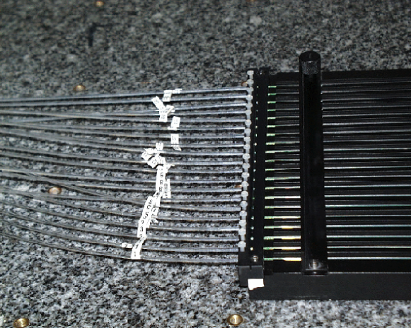
Figure 5: Setup used for coupling clear and WLS fibres.

The second important point is the optical coupling of the test fibres to the clear fibres. The clear and test fibre ends which are in optical contact are diamond cut and polished. This is easily obtained by a dedicated tool. Since no optical interface (grease or optical coupler) is placed between the fibres, their relative geometry must be well reproducible. Fig’s. 2 (b) and 5 show how the coupling between the fibres has been obtained in our system. A carefully machined PVC piece is positioned at the end of the fibre plate. On it, precision holes guide the fibres, clear and WLS, which are kept coaxial till they touch. Clear fibres are held in place by Teflon screws, test fibres are independently held against the plate. The fibre positions can be visually inspected through a groove.

4 Fibre measurement

The first step in the measurement process is the fibre preparation. The diamond cut and polishing of the fibre end facing the clear fibre has alredy been described. The other end of the fibre should not reflect any light. This is obtained by a complete blackening of the fibre end opposite the readout side. The tip of the fibre is cut roughly with scissors at 45 degrees and painted with black oil ink.

The fibres are then numbered, for later reference, placed on the plate and positioned in contact with the clear fibres. We found useful to use a vacuum cleaner to remove residual dust while sliding the fibres in place.

The measurements were then performed in a completely automatic way, under computer control.

After turning on the system we wait for 30 minutes before data taking in order to warm up the electronics and the PMT. Then we start the raster scan of the fibre plate. This is done in coarse steps long the fibre direction (x-axis) and in precise steps across the fibres (y-axis).

• The LED, originally in a fixed starting position (home) is moved to a point 70 cm away from the clear-WLS fibre contact (here the contribution of light escaping from the fibre core and undergoing total reflection at the clad-air boundary is alredy negligibile) and a scan is performed along y in 100$\mu$m steps. At each step a record is taken of the PMT and of the LED currents;

• Subsequently a new scan is performed along y at 10 cm from the first (80 cm from the clear-WLS fibre contact) and the PMT and LED currents are again recorded at each step. The procedure is repeated 12 times, till the end of fibre is reached;

• At the end of the measurement the LED is brought back to its initial position (homing). If, as discussed above, the stepping motors have lost one or a few clock pulses the homing would not be correctly achieved. In such case the measurement would be repeated.

The measurement of 20 fibres takes about 25 minutes and the data recorded are then processed off-line.

Figure 6: Photo current as a function of position during a scanning across 20 fibres (a) and detail from a scanning across a single fibre (b).

At a fixed x, the scan across the fibres produces peaks of photo current, when the LED crosses a fibre. Fig. 6 (a), shows the 20 peaks in a transverse scan corresponding to the 20 fibres under measurement. Each fibre is sampled at several points and its position is thus very well defined. Fig. 6 (b), shows the detail of one of the peaks.

Figure 7: An example of attenuation curve.

The next step is to determine the light yield corresponding to each of the peaks at each position. We have attempted the use of the following variables:

• the maximum of the distribution;

• the area under the peak;

• the maximum of a Gaussian fit to the peak;

• the area of a Gaussian fit to the peak.

We have finally chosen the one which gave the smallest variance in repeated measurements. This turned out to be the maximum of the distribution (ratio between R.M.S. and average about $0.9\%$).

Fig. 7 shows the attenuation curve of a fibre, i.e. the PMT current obtained as just described, as a function of the LED position along the fibre. Fitting an exponential function to the data we extract the parameters needed for the fibre characterization.

4.1 Channel intercalibration

The same fibre measured after placing it in different positions (grooves) on the plate may give different light responses. The relative difference between measurements performed in different grooves cannot be reduced below $20\%$, mainly because of differences among the different clear fibres and their coupling to the PMT. The different positions have thus to be intercalibrated. This is performed following a procedure which is repeated before each new batch of fibres is delivered (2-3 months). The intercalibration is carried out by measuring $20$ times, as described above, a set of $20$ fibres. Each measurement is done after cyclic permutation of the $20$ fibres in the $20$ grooves. We thus know the response of each fibre in all the positions, which allows redundancy in the cross check of the calibration constants. $19$ average calibration constants are obtained as a result of this procedure. The intercalibration procedure also implies that the measurement of a fibre can be reproduced once it is removed from the plate. We find the result to be stable within 1% in repeated intercalibration procedures.

5 Stability and precision

Two important points are:

• the precision of the measurement and the suppression of systematic effects;

• the stability of the system.

Figure 8: Distributions of the attenuation length (a) and light yield (b) of a particular fibre measured after subsequently placing it in each of the 20 grooves of the setup.

We have checked the residual systematic effects by measuring the same fibre after placing it in each of the $20$ positions of the plate. If we have been able to correct for all the effects described above, the attenuation length and the light yield must be independent of the channel number. Fig. 8 (a), shows the attenuation length obtained for the given fibre placed in each of the 20 grooves of the plate. There is no trend or other dependence on the channel number. The precision in the measurement of $\lambda$ is evaluated by the ratio $\sigma_{\lambda}/\bar{\lambda}$ which is equal to $2\%$ Fig. 8 (b), shows the results for the light yield. In this case as well the light yield is independent of the channel number. The ratio $\sigma_{n_{0}}/\bar{n_{0}}=1.3\%$ gives the precision in the measurement of the light yield.

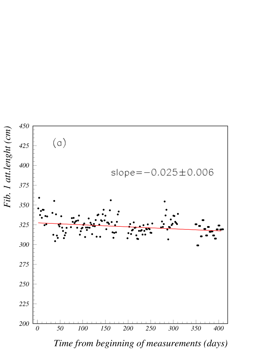
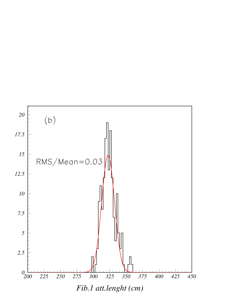
Figure 9: Results of the measurements of attenuation length of reference fibre #1 as a function of time (a). Histogram of results (b).

The fibre characterization process lasted more than one year. During the entire period the stability had to be kept to better than 1%, in order to compare the absolute light yield of the fibres under test. It is not easy to keep an absolute calibration at this level over a period of many months. We thus decided to use two fibres as reference. These were kept fixed in grooves # 1 and # 11 (see figure 6 (a)) and untouched throughout the entire period. The reference fibres are removed from the plate only during the calibration of channels. The light yield measurement was always normalized to the first of the two fibres, while the ratio of the light yield of the two reference fibres was used as a monitor of the system stability. We have checked that the goal of maintaining the stability of the measurement at the level of 1% over one year was achieved.

Fig. 9 shows the results obtained for the attenuation length ($\lambda$) of reference fibre # 1 as a function of time. The measurement shows a slight but significant variation with time (slope $-0.025\pm 0.006$), probably due to a small progressive damage of the fibre. We note that this effect is smaller than the fluctuations of individual measurements, and the overall relative dispersion $\sigma_{\lambda}/\bar{\lambda}=3\%$ is compatible with the precision of a single measurement.

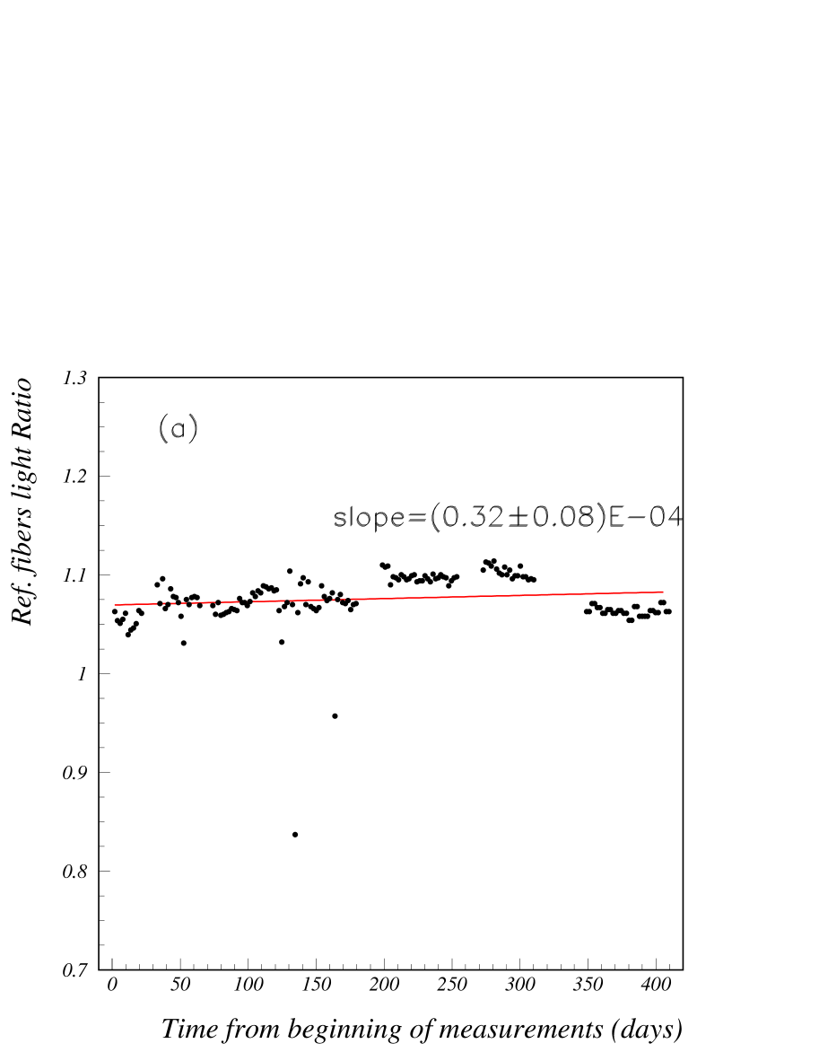
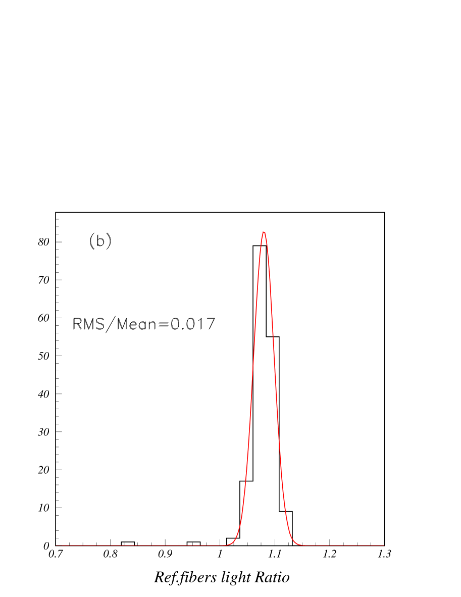
Figure 10: Ratio of the light yield of the references fibres #1 and #11 as a function of time (a). Histogram of results (b).

The ratio of the light yield of reference fibres is shown in Fig. 10 as function of time. It is constant and independent of time, with a relative dispersion: $\sigma_{n_{0}}/\bar{n_{0}}=1.7\%$. The two anomalously low data point seen in fig. 10 are due to an incorrect positionining of fiber #1 on the plate caused by linear thermal expansion. Since the reference fibres were kept fixed on the plate at both ends, temperature variations could result in a bending of the fibres and thus in a wrong measurement. This problem has been solved by rigidly fixing on the plate only the readout end of the fibre, while keeping the other fixed in such a way that it can slide. The measurements have then been repeated. The relative stability of the measurements performed over more than a year turn out to be about 1%.

5.1 Systematics on attenuation length

The measured attenuation length of a fibre is dependent upon the angle under which the light is collected at the fibre end. Light collected at large angles is more likely to correspond to photons undergoing many large-angle reflections at the core-cladding interface thus yielding a shorter attenuation length. The opposite is true of light collected at small angles, corresponding to photons undergoing few reflections. The light which reaches the end of the fibre is a mixture of all these components, and the attenuation length depends on which component is detected. The two extreme cases are:

• light detected at a very small angle to the fibre axis. Here the attenuation length will approximate that of the core material (about 400 cm in our case, where the fibre core has polistyrene as base material);

• light detected at all angles: in this case the light yield will be larger, but the attenuation length shorter (about 250 cm)[10].

In our apparatus the light is collected by the PMT through a single-clad clear fibre, and the optical rays that are impinging on the clear fibre at an angle with the axis larger than the critical value (${19.4}^{\circ})$ escape and cannot thus reach the PMT. As a conseguence the attenuation length that we measure is larger by $30-40\%$ than the one where all the light is collected. When comparing the measured attenuation lengths obtained using different experimental procedures, one has to take into account the details of collection of the light rays by the PMT. We have performed careful studies of this problem, both experimentally [11] and through Montecarlo simulations [12]. The results show that the differences among different measurements agree when the appropriate geometry of light collection is taken into account.

6 Results of the QC for the Tile Calorimeter

This device and the measurement procedure described above has been set up for the quality control of the WLS fibres used by ATLAS in the Tile hadron calorimeter. A fraction of the fibres (75%, corresponding to about 460,000 fibres) have been qualified in our laboratory using this device and following the above procedures.

From the fibres of each preform, we random sampled 18 fibres longer than 2 m. The fibres were prepared, as described above i.e.:

• one end roughly cut and painted with black ink;

• the other end diamond-cut and polished.

The fibres were placed on the plate and coupled to the clear fibres. Fibres 1 and 11 were the reference fibres and were never removed. The scan was performed under computer control and the subsequent off line analysis provided the results for the acceptance procedure. These are shown in Fig. 11 for one of the measured preforms. The “acceptance sheet” in the same figure, shows the attenuation length $\lambda$ and the light yield $n_{0}$ for the 18 fibres under test. Also shown in the lower part of Fig. 11 are some important statistical quantities calculated for this preform together with the acceptance limits of our QC procedure.

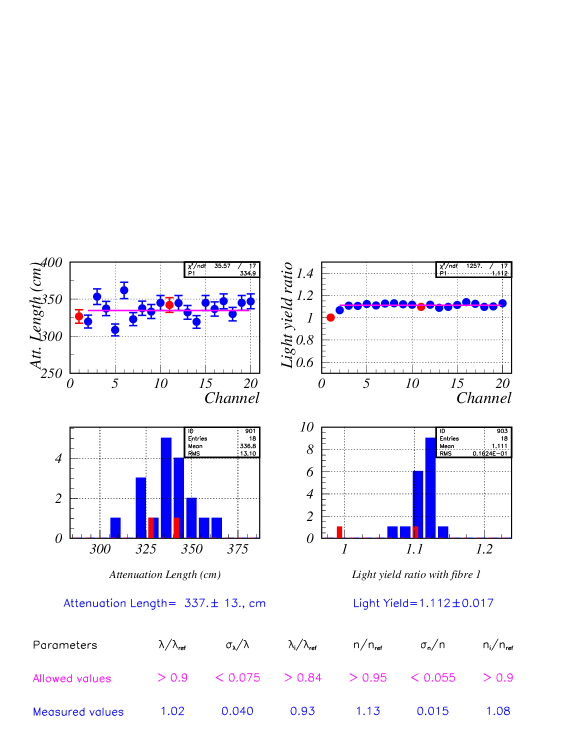
Figure 11: Light yield and attenuation length measured for 18 fibres from one of the measured preforms.

Fig. 12 shows the attenuation length of all measured preforms and their distribution.

Figure 12: Summary of the average attenuation length for 170 tested preforms.

Fig. 13 shows results of the same analysis for the light yield. While the attenuation length was rather constant, the light yield shows an increase in the first part of the production. Having this analysis been carried out on-line, we have been able to notify to the fibre producer the change in this parameter, which they have than been able to correct.

Figure 13: Summary of the average light yield for 170 tested preforms.

7 Conclusions

We have built and put into operation a system to measure in a fast and accurate way the optical parameters of WLS fibres. In this paper we have described the first version of the set up that could measure 20 fibres at a time. The system was later improved to measure 40 fibres at a time.

The resolutions that we obtain using this device are:

• $\Delta n_{0}/n_{0}$=1.5% for the light yield;

• $\Delta\lambda/\lambda$=3% for the attenuation length.

This device was used for the characterization of the fibres that will instrument the hadron calorimeter of ATLAS (Tile Calorimeter), with excellent precision and stability over a long period of measurement.

8 Acknowledgements

We thank our technicians R. Ruberti, F. Mariani for the support provided in the construction of the mechanical parts of the apparatus, and R. Romboli for the help provided during the fibre characterization.

References

- [1] J. Alitti et al., NIM A263(1988) 51.
- [2] D collaboration, “The D Upgrade” FERMILAB Pub-96/357-E(1996).
- [3] KLOE collaboration, “KLOE Detector Tecnical Proposal”, LNF-93/002 (1993).
- [4] D. Acosta et al., NIM A308,481 (1991).
- [5] H1 Collaboration, “Tecnical Proposal to Upgrade the Backward region of the H1 Detector”, PRC 93/02 1993.
- [6] Zeus-Presampler Group, “ A Detector For HERA”,DESY, (1993).
- [7] DELPHI collaboration, preprint CERN-LEPC/92-6.
- [8] ATLAS collaboration, “Technical Proposal for a General Purpose pp experiment at the LHC at CERN”, CERN/LHCC/94-43,1994.
- [9] Tile Calorimeter collaboration, “ Atlas Tile Calorimeter Technical Design Report”, CERN/LHCC/96-42,1996.
- [10] T. Del Prete et al., ATLAS internal note999The ATLAS internal notes can be found at http://weblib.cern.ch in postscript format., TILECAL-NO-089(1996).
- [11] V. Cavasinni et al., to be submitted as an ATLAS internal note.
- [12] V. Cavasinni et al., ATLAS internal note, TILECAL-NO-004 (2000).