Confidence Intervals for Poisson Distribution Parameter

Results of numerical procedure of constructing confidence intervals for parameter of the Poisson distribution of signal events in the presence of background events with known value of parameter of Poisson distribution are presented. It is shown that the used procedure has both the Bayesian and frequentist interpretations. Also the possibility to construct a continuous analogue of the Poisson distribution to search the bounds of confidence intervals for the parameter of the Poisson distribution is discussed.

 
¹  bityukov@mx.ihep.su,Serguei.Bitioukov@cern.ch
²  Institute for Nuclear Research RAS, Moscow.
³  Moscow State Academy of Instrument Engineering and Computer Science, Serpukhov, Russia.

1 Introduction

In paper [1] the unified approach to the construction of confidence intervals and confidence limits for a signal in the background presence, in particular, for Poisson distributions, is proposed. The method is widely used for the presentation of physical results [2] though a number of investigators criticize this approach [3].

Here we use a simple method of constructing confidence intervals for the Poisson distribution parameter for a signal in the presence of background which has the Poisson distribution with the known value of parameter to compare with a conventional procedure  . The method is based on the statement that the probability of true value of the Poisson distribution parameter to be a specified value (in the case of the observed number of events $\hat{x}$) distributes in accordance with a Gamma distribution. It is shown that this statement has both Bayesian and frequentist interpretations. The experimental results often give non-integer values for a number of observed events $\hat{x}$ (for example, after the background subtraction [4]) when the Poisson distribution occurs. That is why there is a necessity to have a procedure for constructing the confidence intervals in this case. The paper offers a generalization of Poisson distribution for a continuous case  . The generalization given here allows one to construct confidence intervals and confidence limits for the Poisson distribution parameter (for integer and real values of a number of observed events) using conventional methods.

In Sect. 2 the interrelation between the frequentist and Bayesian definitions of the confidence interval is shown. The method of constructing confidence intervals for the Poisson distribution parameter for a signal in the presence of background which has the Poisson distribution with the known value of parameter is described in Sect. 3. The results of confidence intervals construction and their comparison with the results of the unified approach are also given in Sect. 3. In Sect. 4 the generalization of Poisson distribution for the continuous case is introduced. The examples of confidence intervals construction for the parameter of the Poisson distribution analogue and for the Poisson distribution parameter using the Gamma distribution are considered in Sect. 5 and in Sect. 6. The main results of the paper are summarized in the Conclusion.

2 The interrelation between frequentist and Bayesian definitions of confidence interval

Let us have a random value $\xi$, taking values from the set of numbers $x\in X$. Consider the two-dimensional function

$$f(x,\lambda)=\displaystyle\frac{\lambda^{x}}{x!}e^{-\lambda},$$

where $x\geq 0$ and $\lambda>0$.

Assume, that the set $X$ includes only the whole numbers, then for each value of $\lambda$ a discrete function $f(x,\lambda)$ describes the distribution of probabilities for the Poisson distribution with the parameter $\lambda$ and a random variable $x$, i.e. $\xi\sim Pois(\lambda)$.

Let us write down the density of Gamma distribution $\Gamma_{a,x+1}$ as

$$f(x,a,\lambda)=\displaystyle\frac{a^{x+1}}{\Gamma(x+1)}e^{-a\lambda}\lambda^{x},$$

where $a$ is a scale parameter, $x+1>0$ is a shape parameter, $\lambda>0$ is a random variable, and $\Gamma(x+1)$ is a Gamma function. Since the $x$ is integer, then $x!=\Gamma(x+1)$. Note that this notation is also used in the case of real $x$. Let us set $a=1$, then for each $x$ a continuous function

$$f(x,\lambda)=\displaystyle\frac{\lambda^{x}}{x!}e^{-\lambda},~{}\lambda>0,~{}x>-1$$

is the density of Gamma distribution $\Gamma_{1,x+1}$ with the scale parameter $a=1$ (see Fig. 1). The mean, mode, and variance of this distribution are given by $x+1,~{}x$, and $x+1$, respectively.

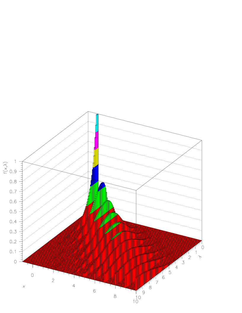
Figure 1: The behaviour of the probability density of the true value of parameter $\lambda$ for the Poisson distribution in case of $x$ observed events versus $\lambda$ and $x$. Here $f(x,\lambda)=\displaystyle\frac{\lambda^{x}}{x!}e^{-\lambda}$ is both the Poisson distribution with the parameter $\lambda$ along the axis $x$ and the Gamma distribution with a shape parameter $x+1$ and a scale parameter 1 along the axis $\lambda$.

Assume that in the experiment with a fixed integral luminosity (i.e. the process under study is considered as a homogeneous process for a given time) the $\hat{x}$ events of a Poisson process are observed. It means that we have an experimental estimation $\hat{\lambda}(\hat{x})$ of the parameter $\lambda$ of the Poisson distribution. We have to construct a confidence interval $(\hat{\lambda}_{1}(\hat{x}),\hat{\lambda}_{2}(\hat{x}))$, covering the true value of the parameter $\lambda$ of the distribution under study with a confidence level $1-\alpha$, where $\alpha$ is a significance level. It is known from the theory of statistics [5], that the mean value of a sample of data is an unbiased estimation of the mean of distribution under study. In our case the sample consists of one  observation $\hat{x}$.

For the discrete Poisson distribution the mean coincides with the estimation of parameter value, i.e. $\hat{\lambda}=\hat{x}$ in our case.

Let us consider the formula

$$P(\lambda|\hat{x})=P(\hat{x}|\lambda)=\displaystyle\frac{\lambda^{\hat{x}}}{\hat{x}!}e^{-\lambda}.$$

This formula (2.4) results from the Bayesian formula [6]

$$P(\lambda|\hat{x})P(\hat{x})=P(\hat{x}|\lambda)P(\lambda)$$

in the assumption that all the possible values of parameter $\lambda$ have equal probability, i.e. $P(\lambda)=const$. In this assumption the probability that unknown parameter $\lambda$ obeys the inequalities $\lambda_{1}~{}\leq~{}\lambda~{}\leq~{}\lambda_{2}$ is given by the evident Bayesian formula

$$P(\lambda_{1}\leq\lambda\leq\lambda_{2}|\hat{x})=P(\lambda_{1}\leq\lambda|\hat{x})-P(\lambda_{2}\leq\lambda|\hat{x})=\int_{\lambda_{1}}^{\lambda_{2}}{P(\lambda|\hat{x})d\lambda},$$

where $P(\lambda|\hat{x})$ is determined by formula (2.4).

Formula (2.6) has also a well defined frequentist meaning. Using the identity 

$$\sum_{i=\hat{x}+1}^{\infty}{\frac{\lambda_{1}^{i}e^{-\lambda_{1}}}{i!}}+\int_{\lambda_{1}}^{\lambda_{2}}{\frac{\lambda^{\hat{x}}e^{-\lambda}}{\hat{x}!}d\lambda}+\sum_{i=0}^{\hat{x}}{\frac{\lambda_{2}^{i}e^{-\lambda_{2}}}{i!}}=1$$

one can rewrite formula (2.6) as

$$P(\lambda_{1}~{}\leq~{}\lambda~{}\leq~{}\lambda_{2}|\hat{x})=1-P(n\leq\hat{x}|\lambda_{2})-P(n>\hat{x}|\lambda_{1})=P(n\leq\hat{x}|\lambda_{1})-P(n\leq\hat{x}|\lambda_{2}),$$

where $P(n\leq\hat{x}|\lambda)=\displaystyle\sum_{n=0}^{\hat{x}}{\frac{\lambda^{n}e^{-\lambda}}{n!}}$ and $P(n>\hat{x}|\lambda)=\displaystyle\sum_{n=\hat{x}+1}^{\infty}{\frac{\lambda^{n}e^{-\lambda}}{n!}}$.

The right hand side of formula (2.8) has a well defined frequentist meaning and it is the definition of the confidence interval in the frequentist approach. Note, that this definition of the confidence interval for the Poisson distribution parameter is self-consistent both for the case $\lambda_{1}=\lambda_{2}$ and for the case $\hat{x}=0$. As an example of the shortest 90% CL confidence interval of such type in case of the observed number of events $\hat{x}=4$ is shown in Fig. 2.

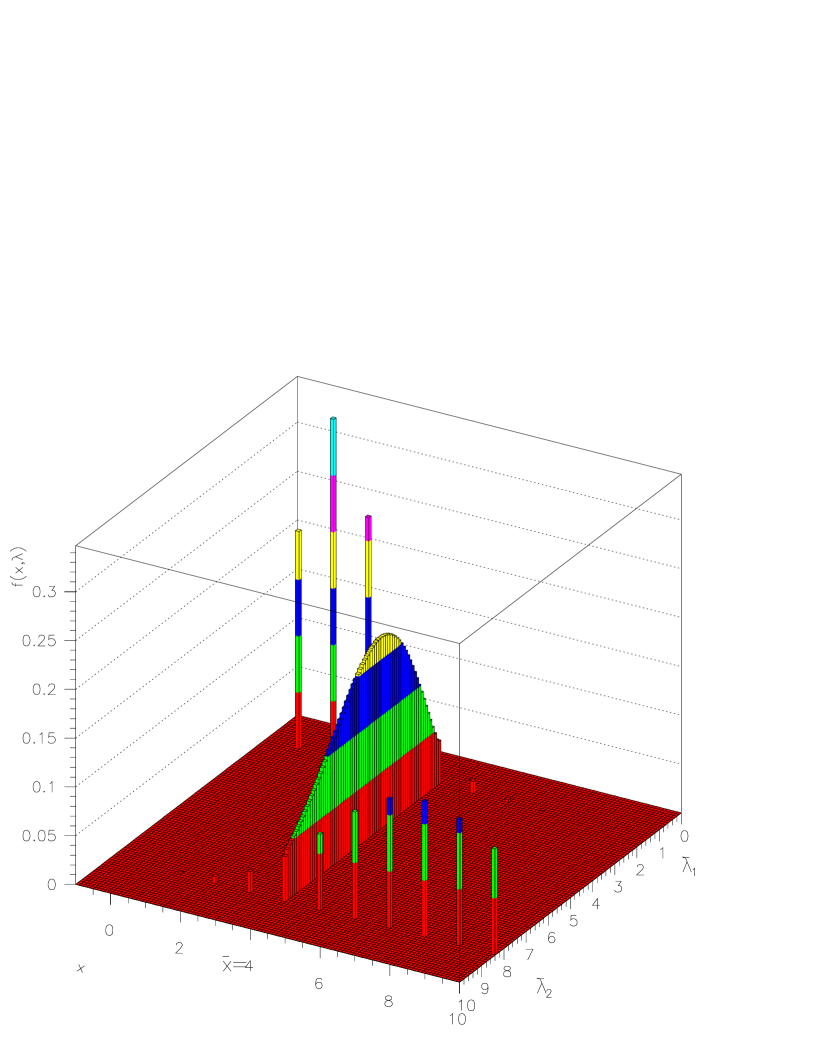
Figure 2: The Poisson distributions $f(x,\lambda)$ for $\lambda$’s determined by the confidence limits $\hat{\lambda}_{1}=1.51$ and $\hat{\lambda}_{2}=8.36$ in case of the observed number of events $\hat{x}=4$ are shown. The probability density of Gamma distribution with a scale parameter $a=1$ and a shape parameter $x+1=\hat{x}+1=5$ is shown within this confidence interval.

In ref. [7] (pp.406-407) the interrelation between the frequentist and Bayesian definitions of confidence interval is shown, nevertheless, the author criticizes the Bayesian approach of the confidence interval determination.

As it is seen from the identity (2.7) the probability of true value of parameter of Poisson distribution to be equal to the value of $\lambda$ in the case of one measurement $\hat{x}$ has probability density of Gamma distribution $\Gamma_{1,1+\hat{x}}$.

Correspondingly, in the case of $m$ measurements $\hat{x}_{1},\hat{x}_{2},\dots,\hat{x}_{m}$ of the random values $\xi_{1},\xi_{2},...,\xi_{m}$, where $\xi_{i}\sim Pois(\lambda)$ for $i=1,2,\dots,m$, the probability of true value of parameter of Poisson distribution to be equal to the value of $\lambda$ has probability density of Gamma distribution $\Gamma_{m,1+\sum_{i=1}^{m}{\hat{x}_{i}}}$.

3 The method of confidence intervals construction

Let us consider the Poisson distribution with two components: Signal component with a parameter $\lambda_{s}$ and background component with a parameter $\lambda_{b}$, where $\lambda_{b}$ is known. To construct confidence intervals for the parameter $\lambda_{s}$ of a signal in the case of observed value $\hat{x}$, we must find the distribution $P(\lambda_{s}|\hat{x})$.

Firstly let us consider the simplest case $\hat{x}=\hat{s}+\hat{b}=1$. Here $\hat{s}$ is the number of signal events and $\hat{b}$ is the number of background events among the observed $\hat{x}$ events.

The $\hat{b}$ can be equal to 0 and 1. We know that the $\hat{b}$ is equal to 0 with probability

$$p_{0}=P(\hat{b}=0)=\displaystyle\frac{\lambda_{b}^{0}}{0!}e^{-\lambda_{b}}=e^{-\lambda_{b}}$$

and the $\hat{b}$ is equal to 1 with probability

$$p_{1}=P(\hat{b}=1)=\displaystyle\frac{\lambda_{b}^{1}}{1!}e^{-\lambda_{b}}=\lambda_{b}e^{-\lambda_{b}}.$$

Correspondingly, $P(\hat{b}=0|\hat{x}=1)=P(\hat{s}=1|\hat{x}=1)=\displaystyle\frac{p_{0}}{p_{0}+p_{1}}$ and $P(\hat{b}=1|\hat{x}=1)=P(\hat{s}=0|\hat{x}=1)=\displaystyle\frac{p_{1}}{p_{0}+p_{1}}$.

It means that the distribution of $P(\lambda_{s}|\hat{x}=1)$ is equal to the sum of distributions

$$P(\hat{s}=1|\hat{x}=1)\Gamma_{1,2}+P(\hat{s}=0|\hat{x}=1)\Gamma_{1,1}=\displaystyle\frac{p_{0}}{p_{0}+p_{1}}\Gamma_{1,2}+\displaystyle\frac{p_{1}}{p_{0}+p_{1}}\Gamma_{1,1},$$

where $\Gamma_{1,1}$ is the Gamma distribution with the probability density $P(\lambda_{s}|\hat{s}=0)=\displaystyle e^{-\lambda_{s}}$ and $\Gamma_{1,2}$ is the Gamma distribution with the probability density $P(\lambda_{s}|\hat{s}=1)=\displaystyle\lambda_{s}e^{-\lambda_{s}}$. As a result, we have

$$P(\lambda_{s}|\hat{x}=1)=\displaystyle\frac{\lambda_{s}+\lambda_{b}}{1+\lambda_{b}}\displaystyle e^{-\lambda_{s}}.$$

Using formula (3.4) for $P(\lambda_{s}|\hat{x}=1)$ and formula (2.8), we construct the shortest confidence interval of any confidence level in a trivial way.

In this manner we can construct the distribution of $P(\lambda_{s}|\hat{x})$ for any values of $\hat{x}$ and $\lambda_{b}$. As a result, we have obtained the known formula [8, 9]

$$P(\lambda_{s}|\hat{x})=\displaystyle\frac{(\lambda_{s}+\lambda_{b})^{\hat{x}}}{\hat{x}!\displaystyle\sum_{i=0}^{\hat{x}}{\lambda_{b}^{i}\over{i!}}}\displaystyle e^{-\lambda_{s}}.$$

The numerical results for the confidence intervals and the results of paper [1] are compared in Table 1 and Table 2.

Table 1: 90% C.L. intervals for the Poisson signal mean $\lambda_{s}$, for total events observed $\hat{x}$, for known mean background $\lambda_{b}$ ranging from 0 to 2. Comparison between the results of ref.[1] and the results from the present paper.

$\hat{x}\backslash\lambda_{b}$	0.0 ref.[1]	0.0	1.0 ref.[1]	1.0	2.0 ref.[1]	2.0
0	0.00, 2.44	0.00, 2.30	0.00, 1.61	0.00, 2.30	0.00, 1.26	0.00, 2.30
1	0.11, 4.36	0.09, 3.93	0.00, 3.36	0.00, 3.27	0.00, 2.53	0.00, 3.00
2	0.53, 5.91	0.44, 5.48	0.00, 4.91	0.00, 4.44	0.00, 3.91	0.00, 3.88
3	1.10, 7.42	0.93, 6.94	0.10, 6.42	0.00, 5.71	0.00, 5.42	0.00, 4.93
4	1.47, 8.60	1.51, 8.36	0.74, 7.60	0.51, 7.29	0.00, 6.60	0.00, 6.09
5	1.84, 9.99	2.12, 9.71	1.25, 8.99	1.15, 8.73	0.43, 7.99	0.20, 7.47
6	2.21,11.47	2.78,11.05	1.61,10.47	1.79,10.07	1.08, 9.47	0.83, 9.01
7	3.56,12.53	3.47,12.38	2.56,11.53	2.47,11.38	1.59,10.53	1.49,10.37
8	3.96,13.99	4.16,13.65	2.96,12.99	3.18,12.68	2.14,11.99	2.20,11.69
9	4.36,15.30	4.91,14.95	3.36,14.30	3.91,13.96	2.53,13.30	2.90,12.94
10	5.50,16.50	5.64,16.21	4.50,15.50	4.66,15.22	3.50,14.50	3.66,14.22
20	13.55,28.52	13.50,28.33	12.55,27.52	12.53,27.34	11.55,26.52	11.53,26.34

Table 2: 90% C.L. intervals for the Poisson signal mean $\lambda_{s}$, for total events observed $\hat{x}$, for known mean background $\lambda_{b}$ ranging from 6 to 15. Comparison between the results of ref.[1] and the results from the present paper.

$\hat{x}\backslash\lambda_{b}$	6.0 ref.[1]	6.0	12.0 ref.[1]	12.0	15.0 ref.[1]	15.0
0	0.00, 0.97	0.00, 2.30	0.00, 0.92	0.00, 2.30	0.00, 0.92	0.00, 2.30
1	0.00, 1.14	0.00, 2.63	0.00, 1.00	0.00, 2.48	0.00, 0.98	0.00, 2.45
2	0.00, 1.57	0.00, 3.01	0.00, 1.09	0.00, 2.68	0.00, 1.05	0.00, 2.61
3	0.00, 2.14	0.00, 3.48	0.00, 1.21	0.00, 2.91	0.00, 1.14	0.00, 2.78
4	0.00, 2.83	0.00, 4.04	0.00, 1.37	0.00, 3.16	0.00, 1.24	0.00, 2.98
5	0.00, 4.07	0.00, 4.71	0.00, 1.58	0.00, 3.46	0.00, 1.32	0.00, 3.20
6	0.00, 5.47	0.00, 5.49	0.00, 1.86	0.00, 3.80	0.00, 1.47	0.00, 3.46
7	0.00, 6.53	0.00, 6.38	0.00, 2.23	0.00, 4.19	0.00, 1.69	0.00, 3.74
8	0.00, 7.99	0.00, 7.35	0.00, 2.83	0.00, 4.64	0.00, 1.95	0.00, 4.06
9	0.00, 9.30	0.00, 8.41	0.00, 3.93	0.00, 5.15	0.00, 2.45	0.00, 4.42
10	0.22,10.50	0.02, 9.53	0.00, 4.71	0.00, 5.73	0.00, 3.00	0.00, 4.83
20	7.55,22.52	7.53,22.34	2.23,16.52	1.70,16.08	0.00,13.52	0.00,12.31

It should be noted that in our approach the dependence of the confidence intervals width for the parameter $\lambda_{s}$ on the value of $\lambda_{b}$ in the case $\hat{x}=0$ is absent. For $\hat{x}=0$ the method proposed in ref. [10] also gives a 90% upper limit independent of $\lambda_{b}$. This dependence is also absent in the Bayesian approach [8, 11].

4 The Generalization of Discrete Poisson Distribution for the Continuous Case

Let us consider the case when $x\in X$ are the real values and denote $x!=\Gamma(x+1)$, then we can consider the function

$$f(x,\lambda)=\displaystyle\frac{\lambda^{x}}{x!}e^{-\lambda}$$

as a continuous two-dimensional function. Fig. 3 shows the surface described by this function. Smooth behaviour of this function along $x$ and $\lambda$ (see Fig. 4) allows one to assume that there is such a function $\l(\lambda)>-1$, that

$$\int_{l(\lambda)}^{\infty}{f(x,\lambda)dx}=1$$

for the given value of $\lambda$. It means that in this way we introduce a continued analogue of Poisson distribution with the probability density $f(x,\lambda)=\displaystyle\frac{\lambda^{x}}{x!}e^{-\lambda}$ over the area of the function definition, i.e. for $x\geq l(\lambda)$ and $\lambda>0$.

Figure 3: The behaviour of the function $f(x,\lambda)$ versus $\lambda$ and $x$.

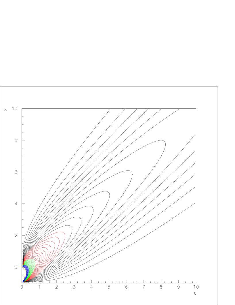
Figure 4: Two-dimensional representation of the function $f(x,\lambda)$ versus $\lambda$ and $x$ for the values $f(x,\lambda)<1$.

The values of the function $f(x,\lambda)$ for integer $x$ coincide with corresponding magnitudes in the probabilities distribution of discrete Poisson distribution. Dependences of the values of function $\l(\lambda)$, the means and the variances for the suggested distribution on $\lambda$ have been calculated by using the programme DGQUAD from the library CERNLIB [12] and the results are presented in Table 3. This Table shows that the series of properties of Poisson distribution $(E\xi=\lambda,D\xi=\lambda)$ take place only when the value of the parameter $\lambda>3$.

Table 3: The function $l(\lambda)$, mean and variance versus $\lambda$.

$\lambda$	$l(\lambda)$	mean $(E\xi)$	variance $(D\xi)$
0.001	-0.297	-0.138	0.024
0.002	-0.314	-0.137	0.029
0.005	-0.340	-0.130	0.040
0.010	-0.363	-0.120	0.052
0.020	-0.388	-0.100	0.071
0.050	-0.427	-0.051	0.113
0.100	-0.461	0.018	0.170
0.200	-0.498	0.142	0.272
0.300	-0.522	0.256	0.369
0.400	-0.539	0.365	0.464
0.500	-0.553	0.472	0.559
0.600	-0.564	0.577	0.653
0.700	-0.574	0.681	0.748
0.800	-0.582	0.785	0.844
0.900	-0.590	0.887	0.939
1.00	-0.597	0.989	1.035
1.50	-0.622	1.495	1.521
2.00	-0.639	1.998	2.012
2.50	-0.650	2.499	2.506
3.00	-0.656	3.000	3.003
3.50	-0.656	3.500	3.501
4.00	-0.647	4.000	3.999
4.50	-0.628	4.500	4.498
5.00	-0.593	5.000	4.997
5.50	-0.539	5.500	5.497
6.00	-0.466	6.000	5.996
6.50	-0.373	6.500	6.495
7.00	-0.262	7.000	6.995
7.50	-0.135	7.500	7.494
8.00	0.000	8.000	7.993
8.50	0.000	8.500	8.496
9.00	0.000	9.000	8.997
9.50	0.000	9.500	9.498
10.0	0.000	10.00	9.999

It is appropriate at this point to say that

$$\int_{0}^{\infty}{f(x,\lambda)dx}=\displaystyle\int_{0}^{\infty}{\frac{\lambda^{x}e^{-\lambda}}{\Gamma(x+1)}dx}=e^{-\lambda}\nu(\lambda).$$

The function

$$\nu(\lambda)=\displaystyle\int_{0}^{\infty}{\frac{\lambda^{x}}{\Gamma(x+1)}dx}$$

is well known and, according to ref. [13],

$$\nu(\lambda)=\displaystyle\sum_{n=-N}^{\infty}{\frac{\lambda^{n}}{\Gamma(n+1)}}+O(|\lambda|^{-N-0.5})=e^{\lambda}+O(|\lambda|^{-N})$$

if $\lambda\rightarrow\infty,~{}~{}|arg\lambda|\leq\frac{\pi}{2}$ for any integer $N$. Nevertheless we have to use the function $l(\lambda)$ in our calculations in Sect. 5 and Sect. 6. We consider it as a mathematical trick to illustrate a possibility of constructing confidence intervals numerically for the real value $\hat{x}$.

Another approaches are also possible. At first, if we introduce a prior $\displaystyle g(\lambda)=\frac{e^{\lambda}}{\nu(\lambda)}$, then we have equality $\displaystyle\int_{0}^{\infty}{g(\lambda)f(x,\lambda)dx}=1$ by natural way. Also we can numerically transform the function $f(x,\lambda)$ in the interval $x\in(0,1)$ so that

$$\int_{0}^{\infty}{f(x,\lambda)dx}=1,~{}~{}E\xi=\displaystyle\int_{0}^{\infty}{xf(x,\lambda)dx}=\lambda,~{}~{}D\xi=\displaystyle\int_{0}^{\infty}{(x-E\xi)^{2}f(x,\lambda)dx}=\lambda$$

for any $\lambda$. In these cases we can construct the confidence interval without introducing $l(\lambda)$.

Let us construct the central confidence interval for the continued analogue of Poisson distribution using the function $l(\lambda)$.

5 The Central Confidence Intervals for the Continued Analogue of Poisson Distribution.

As we have noticed, for the discrete Poisson distribution the mean coincides with the estimation of parameter value, i.e. $\hat{\lambda}=\hat{x}$. This is not true for a small value of $\lambda$ in the considered case (see Table 3). That is why in order to find the estimation of $\hat{\lambda}(\hat{x})$ for a small value $\hat{x}$ it is necessary to introduce the correction in accordance with Table 3. Let us construct the central confidence intervals using a conventional method assuming that

$$\int_{\hat{x}}^{\infty}{f(x,\hat{\lambda}_{1})dx}=\frac{\alpha}{2}$$

for the lower bound $\hat{\lambda}_{1}$ and

$$\int_{l(\hat{\lambda}_{2})}^{\hat{x}}{f(x,\hat{\lambda}_{2})dx}=\frac{\alpha}{2}$$

for the upper bound $\hat{\lambda}_{2}$ of the confidence interval.

Fig. 5 shows the introduced distributions (Sect. 4) with parameters defined by the bounds of confidence interval $(\hat{\lambda}_{1}=1.638,\hat{\lambda}_{2}=8.493)$ for $\hat{x}=\hat{\lambda}=4$ and the Gamma distribution with parameters $a=1$, $x+1=\hat{x}+1=5$.

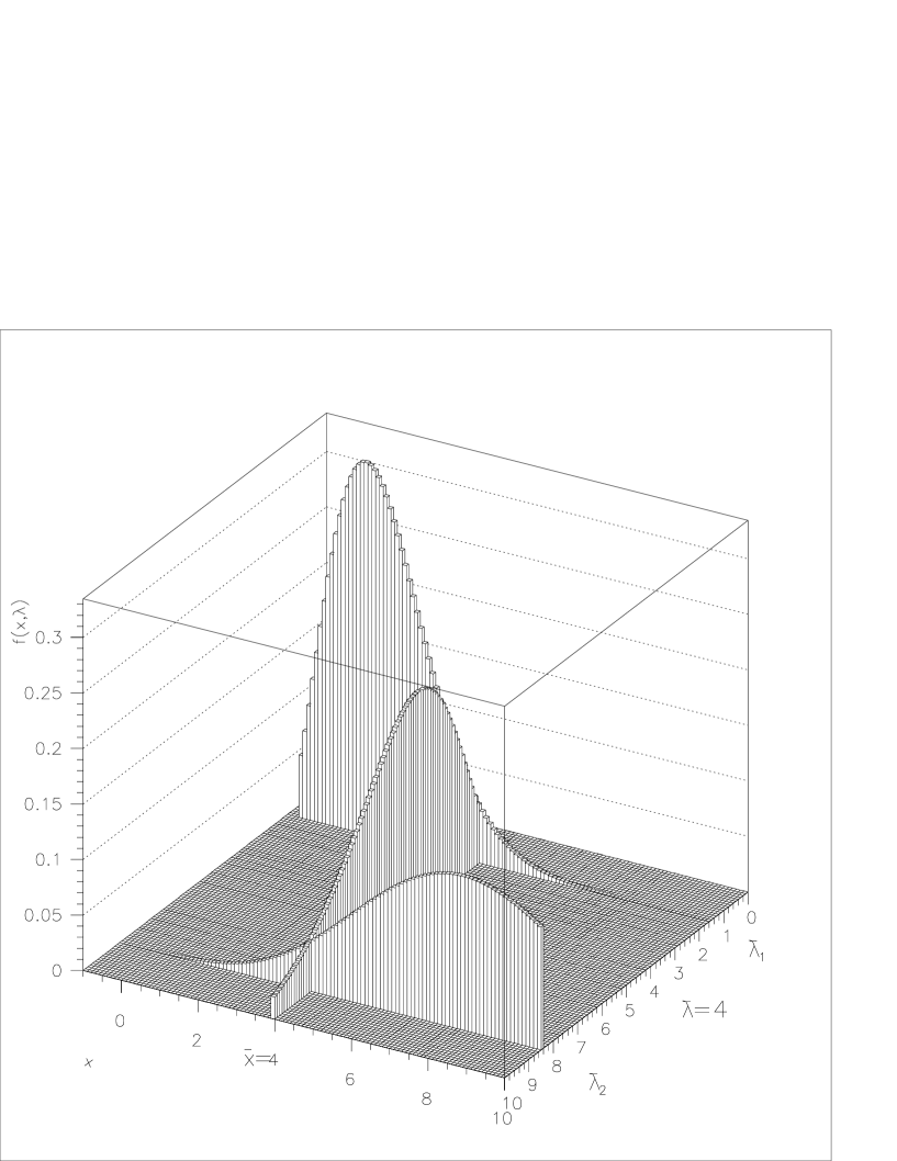
Figure 5: The probability densities $f(x,\lambda)$ of continued analogue Poisson distribution for $\lambda$’s determined by the confidence limits $\hat{\lambda}_{1}$ and $\hat{\lambda}_{2}$ in case of the observed number of events $\hat{x}=4$ and the probability density of Gamma distribution with parameters $a=1$ and $x+1=\hat{x}+1=5$.

The bounds of confidence interval with a 90% confidence level for the parameter of continued analogue of Poisson distribution for different observed values $\hat{x}$ (first column) were calculated and are given in the second column of Table 4.

Table 4: 90% C.L. intervals for the Poisson signal mean $\lambda$ for total events observed $\hat{x}$.

	bounds	(Section 5)	bounds	(Section 6)
$\hat{x}$	$\hat{\lambda}_{1}$	$\hat{\lambda}_{2}$	$\hat{\lambda}_{1}$	$\hat{\lambda}_{2}$
0.000	0.121E-08	2.052	0.0	2.303
0.001	0.205E-08	2.054	0.0	2.304
0.002	0.292E-08	2.056	0.0	2.306
0.005	0.666E-08	2.061	0.0	2.311
0.02	0.218E-06	2.098	0.0	2.337
0.05	0.765E-05	2.166	1.66E-05	2.389
0.10	0.137E-03	2.275	2.23E-05	2.474
0.20	0.186E-02	2.490	6.65E-05	2.642
0.30	0.696E-02	2.692	1.49E-04	2.806
0.40	0.161E-01	2.891	2.60E-03	2.969
0.50	0.295E-01	3.084	5.44E-03	3.129
0.60	0.466E-01	3.269	1.35E-02	3.290
0.70	0.673E-01	3.450	2.63E-02	3.452
0.80	0.911E-01	3.629	4.04E-02	3.611
0.90	0.1179	3.804	6.12E-02	3.773
1.0	0.1473	3.977	8.49E-02	3.933
1.5	0.3257	4.800	0.2391	4.718
2.0	0.5429	5.582	0.4410	5.479
2.5	0.7896	6.340	0.6760	6.220
3.0	1.056	7.076	0.9284	6.937
3.5	1.340	7.792	1.219	7.660
4.0	1.638	8.493	1.511	8.358
4.5	1.946	9.188	1.820	9.050
5.0	2.264	9.869	2.120	9.714
5.5	2.590	10.55	2.453	10.39
6.0	2.924	11.21	2.775	11.05
6.5	3.264	11.87	3.126	11.72
7.0	3.609	12.53	3.473	12.38
7.5	3.961	13.18	3.808	13.01
8.0	4.316	13.82	4.160	13.65
8.5	4.677	14.46	4.532	14.30
9.0	5.041	15.10	4.905	14.95
9.5	5.406	15.73	5.252	15.56
10.	5.779	16.36	5.640	16.21
20.	13.65	28.49	13.50	28.33

As a result (Table 4) the suggested approach allows one to construct confidence intervals for any real and integer values of the observed number of events for the values of parameter $\lambda>3$. Table 4 illustrates that the left bound of central confidence intervals is not equal to zero for small $\hat{x}$. It shows that in this case a central confidence interval is not suitable.

To anticipate a little, note that 90% of the area of Gamma distributions with the parameter $x+1=\hat{x}+1$ are contained inside the constructed 90% confidence intervals for the observed value $\hat{x}$. However, for small values of $\hat{x}$ we have got values of the area close to 88%, i.e. less than 90%.

The main goal of the proposed construction is to demonstrate a possibility of using a continuous two-dimensional function (4.1) for the construction of confidence intervals in a frequentist meaning.

6 Confidence Intervals for the Parameter of Poisson Distribution in case of the real value of observed number of events.

As follows from formulae $(2.7)$ and $(2.8)$ (see Figs. 1-2) the probability of true value of parameter of Poisson distribution to be $\lambda$ in case of observed integer value $\hat{x}\geq 0$ distributes in accordance with the Gamma distribution with the parameters $a=1$ and $x+1=\hat{x}+1$, i.e. according to formula $(2.4)$

$P(\lambda|\hat{x})=\displaystyle\frac{\lambda^{\hat{x}}}{\hat{x}!}e^{-\lambda}$.

The possibility of constructing the continued analogue of Poisson distribution suggests to assume that the Gamma distribution of true value of the parameter $\lambda$ takes place in case of the real value $\hat{x}\geq 0$ too (Figs. 3-5). This supposition allows one to choose a confidence interval (for example) of a minimum length of all the possible confidence intervals of the given confidence level. The bounds of minimum length area, containing 90% of the corresponding area of probability density of Gamma distribution, were found numerically for several values of $\hat{x}$. We took into account that $x=\hat{x}$ and required that $\lambda_{1}\geq 0$. The results are presented in the third column of Table 4.

7 Conclusion

In the paper the frequentist approach to construct the confidence interval for Poisson distribution parameter is considered. It is shown that the formula $P(\lambda_{1}~{}\leq~{}\lambda~{}\leq~{}\lambda_{2}|\hat{x})=P(n\leq\hat{x}|\lambda_{1})-P(n\leq\hat{x}|\lambda_{2})$ is a self-consistent definition of the confidence interval in this case. It means that the probability of true value of parameter of Poisson distribution to be equal to the value of $\lambda$ in the case of $m$ measurements $\hat{x}_{1},\hat{x}_{2},\dots,\hat{x}_{m}$ has probability density of Gamma distribution $\Gamma_{m,1+\sum_{i=1}^{m}{\hat{x}_{i}}}$. The results of constructing the frequentist confidence intervals for the parameter $\lambda_{s}$ of Poisson distribution for the signal in the presence of background with the known value of parameter $\lambda_{b}$ are presented. It is shown that the used procedure has both the Bayesian and frequentist interpretations. Also the attempt of introducing a continued analogue of Poisson distribution for the construction of confidence intervals for the parameter $\lambda$ of Poisson distribution is discussed. Two approaches are considered. Confidence intervals for different integer and real values of the number of the observed events for the Poisson process in the experiment with a given integral luminosity are constructed.

We are grateful to V.A. Matveev and V.F. Obraztsov for the interest to this work and for valuable comments. We wish to thank S.S. Bityukov, A.V. Dorokhov, V.A. Litvine and V.N. Susoikin for useful discussions. We would like to thank E.A. Medvedeva and E.N. Gorina for the help in preparing the article.

This work has been supported by grant INTAS-CERN 99-377 and grant INTAS-CERN 00-440.

References

- [1] G.J. Feldman and R.D. Cousins, Unified approach to the classical statistical analysis of small signal, Phys.Rev. D 57 (1998) 3873-3889
- [2] D.E. Groom et al., Review of particle physics. J. Bartels, D. Haidt and A. Zichichi Eds., Eur.Phys.J. C 3 (1998) 198-199.
- [3] as an example, G. Zech, Classical and Bayesian Confidence Limits. in Proc. of 1st Workshop on Confidence Limits, James, F., Lyons, L., and Perrin, Y. Eds., CERN 2000-005, Geneva, Switzerland, (2000) 141-154.
- [4] D. Cronin-Hennessy et al., Observation of and and Evidence for Phys.Rev.Lett. D 85 (2000) 515.
- [5] as an example, Handbook of Probability Theory and Mathematical Statistics (in Russian). V.S. Korolyuk Ed., Kiev, “Naukova Dumka” (1978).
- [6] L.J. Rainwater and C.S. Wu, Nucleonics 1 (1947) 60
- [7] R.D. Cousins, Why isn’t every physicist a Baysian ? Am.J.Phys 63 (1995) 398-410.
- [8] G. D’Agostini, Bayesian Reasoning in High-Energy Physics: Principles and Applications. Yellow Report CERN 99-03, Geneva, Switzerland, (1999) p.95; also D’Agostini G., e-print arXiv: hep-ph/9512295, (December 1995), p.70.
- [9] G. Zech, Upper Limits in Experiments with Background or Measurement Errors. Nucl.Inst.&Meth. A 277 (1989) 608-610.
- [10] B.P. Roy and M.B. Woodroofe, Improved Probability Method for Estimating Signal in the Presence of Background. Phys.Rev. D 60 (1999) 053009.
- [11] O. Helene, Upper Limit of Peak Area. Nucl.Inst.&Meth. A212 (1983) 319-322.
- [12] CERNLIB, CERN PROGRAM LIBRARY, Short Writeups, (CERN, Geneva, Switzerland, Edition - June 1996)
- [13] M. Bateman, Higher Transcendental Functions. Vol. 3, A. Erdlyi Ed., (McGraw-Hill Book Company Inc., 1955) 217-224