\begin{picture}(150.0,180.0)\par{\sfb\put(0.0,40.0){\Huge TESLA} \put(0.0,15.0){\begin{minipage}{398.33858pt} \LARGE\bf\begin{flushleft}{\sfb\LARGE The Superconducting Electron Positron \\ Linear Collider with an Integrated\\ X-Ray Laser Laboratory\\ }\end{flushleft}\end{minipage}} \put(0.0,-10.0){\Huge Technical Design Report} \put(5.0,-25.0){\LARGE Part VI: Appendices} \put(5.0,-37.0){\LARGE Chapter 1: Photon Collider at TESLA } \put(15.0,-130.0){\includegraphics[height=227.62204pt]{part61.ps}} \put(-5.0,-150.0){{\sfb\bf\large DESY-2001-011, ECFA-2001-209}} \put(-5.0,-155.0){{\sfb\bf\large TESLA-2001-23, TESLA-FEL-2001-05}} \par\put(131.0,-150.0){\sfb\large March} \put(135.0,-155.0){\sfb\large 2001}} \end{picture}

\begin{picture}(150.0,180.0)\par{\sfb\put(0.0,55.0){\Huge TESLA} \par\put(0.0,40.0){\Huge Technical Design Report} } \par{\large\put(-5.0,15.0){{\bf\Large PART I: Executive Summary }} \put(25.0,7.0){Editors: \begin{minipage}[t]{284.52756pt}{F.Richard, J.R.Schneider, D.Trines, A.Wagner}\end{minipage}} \put(-5.0,-5.0){{\bf\Large PART II: The Accelerator}} \put(25.0,-13.0){Editors: \begin{minipage}[t]{256.0748pt}{R.Brinkmann, K.Fl\"{o}ttmann, J.Rossbach,\hfil P.Schm\"{u}ser, N.Walker, H.Weise}\end{minipage}} \put(-5.0,-25.0){{\bf\Large PART III: Physics at an e${}^{+}$e${}^{-}$ Linear Collider}} \put(25.0,-33.0){Editors: \begin{minipage}[t]{284.52756pt}{R.D.Heuer, D.Miller, F.Richard, P.Zerwas}\end{minipage} } \put(-5.0,-45.0){{\bf\Large PART IV: A Detector for TESLA}} \put(25.0,-53.0){Editors: \begin{minipage}[t]{284.52756pt}{T.Behnke, S.Bertolucci, R.D.Heuer, R.Settles }\end{minipage}} \put(-5.0,-65.0){{\bf\Large PART V: The X-Ray Free Electron Laser Laboratory}} \put(25.0,-73.0){Editors: \begin{minipage}[t]{284.52756pt}{G.Materlik, T.Tschentscher}\end{minipage}} \put(-5.0,-85.0){{\bf\Large PART VI: Appendices}} \put(25.0,-93.0){Editors: \begin{minipage}[t]{284.52756pt}{ R.Klanner\\ Chapter 1: V.Telnov\\ Chapter 2: U.Katz, M.Klein, A.Levy\\ Chapter 3: R.Kaiser, W.D.Nowak\\ Chapter 4: E.DeSanctis, J.-M.Laget, K.Rith }\end{minipage}} } \end{picture}

\begin{picture}(150.0,180.0)\par\put(0.0,30.0){\sfb\LARGE Part VI} \put(0.0,15.0){\sfb\LARGE Chapter 1: Photon Collider at TESLA } \par\put(0.0,0.0){\sfb\Large Editor: V. Telnov} \par\end{picture}

Chapter 0 The Photon Collider at TESLA

B. Badelek⁴³, C. Blöchinger⁴⁴, J. Blümlein¹², E. Boos²⁸, R. Brinkmann¹², H. Burkhardt¹¹, P. Bussey¹⁷, C. Carimalo³³, J. Chyla³⁴, A.K. Çiftçi⁴, W. Decking¹², A. De Roeck¹¹, V. Fadin¹⁰, M. Ferrario¹⁵, A. Finch²⁴, H. Fraas⁴⁴, F. Franke⁴⁴, M. Galynskii²⁷, A. Gamp¹², I. Ginzburg³¹, R. Godbole⁶, D.S. Gorbunov²⁸, G. Gounaris³⁹, K. Hagiwara²², L. Han¹⁹, R.-D. Heuer¹⁸, C. Heusch³⁶, J. Illana¹², V. Ilyin²⁸, P. Jankowski⁴³, Yi Jiang¹⁹, G. Jikia¹⁶, L. Jönsson²⁶, M. Kalachnikow⁸, F. Kapusta³³, R. Klanner^12,18, M. Klasen¹², K. Kobayashi⁴¹, T. Kon⁴⁰, G. Kotkin³⁰, M. Krämer¹⁴, M. Krawczyk⁴³, Y.P. Kuang⁷, E. Kuraev¹³, J. Kwiecinski²³, M. Leenen¹², M. Levchuk²⁷, W.F. Ma¹⁹, H. Martyn¹, T. Mayer⁴⁴, M. Melles³⁵, D.J Miller²⁵, S. Mtingwa²⁹, M. Mühlleitner¹², B. Muryn²³, P.V. Nickles⁸, R. Orava²⁰, G. Pancheri¹⁵, A. Penin¹², A. Potylitsyn⁴², P. Poulose⁶, T. Quast⁸, P. Raimondi³⁷, H. Redlin⁸, F. Richard³², S.D. Rindani², T. Rizzo³⁷, E. Saldin¹², W. Sandner⁸, H. Schönnagel⁸, E. Schneidmiller¹², H.J. Schreiber¹², S. Schreiber¹², K.P. Schüler¹², V. Serbo³⁰, A. Seryi³⁷, R. Shanidze³⁸, W. Da Silva³³, S. Söldner-Rembold¹¹, M. Spira³⁵, A.M. Stasto²³, S. Sultansoy⁵, T. Takahashi²¹, V. Telnov^10,12, A. Tkabladze¹², D. Trines¹², A. Undrus⁹, A. Wagner¹², N. Walker¹², I. Watanabe³, T. Wengler¹¹, I. Will^8,12, S. Wipf¹², Ö. Yavaş⁴, K. Yokoya²², M. Yurkov¹², A.F. Zarnecki⁴³, P. Zerwas¹², F. Zomer³².

  ¹ RWTH Aachen, Germany
  ² PRL, Ahmedabad, India
  ³ Akita KeizaiHoka University, Japan
  ⁴ Ankara University, Turkey
  ⁵ Gazi University, Ankara, Turkey
  ⁶ Indian Institute of Science, Bangalore, India
  ⁷ Tsinghua University, Beijing, P.R. China
  ⁸ Max–Born–Institute, Berlin, Germany
  ⁹ BNL, Upton, USA
¹⁰ Budker INP, Novosibirsk, Russia
¹¹ CERN, Geneva, Switzerland
¹² DESY, Hamburg and Zeuthen, Germany
¹³ JINR, Dubna, Russia
¹⁴ University of Edinburgh, UK
¹⁵ INFN-LNF, Frascati, Italy
¹⁶ Universität Freiburg, Germany
¹⁷ University of Glasgow, UK
¹⁸ Universität Hamburg, Germany
¹⁹ CUST, Hefei, P.R.China
²⁰ University of Helsinki, Finland
²¹ Hiroshima University, Japan
²² KEK, Tsukuba, Japan
²³ INP, Krakow, Poland
²⁴ University of Lancaster, UK
²⁵ UCL, London, UK
²⁶ University of Lund, Sweden
²⁷ Inst. of Physics, Minsk, Belarus
²⁸ Moscow State University, Russia
²⁹ N.Carolina Univ., USA
³⁰ Novosibirsk State University, Russia
³¹ Inst. of Math., Novosibirsk, Russia
³² LAL, Orsay, France
³³ Université de Paris VI–VII, France
³⁴ IP, Prague, Czech Republic
³⁵ PSI, Villingen, Switzerland
³⁶ UCSC, Santa Cruz, USA
³⁷ SLAC, Stanford, USA
³⁸ Tbilisi State University, Georgia
³⁹ University of Thessaloniki, Greece
⁴⁰ Seikei University, Tokyo, Japan
⁴¹ Sumimoto Heavy Industries, Tokyo, Japan
⁴² Polytechnic Institute, Tomsk, Russia
⁴³ Warsaw University, Poland
⁴⁴ Universität Würzburg, Germany

Contents

1. 0 The Photon Collider at TESLA
   1. 1 Introduction
      1. 1 Principle of a photon collider
      2. 2 Particle production in high energy $\gamma\gamma$, $\gamma$e collisions
   2. 2 The Physics
      1. 1 Possible scenarios
      2. 2 Higgs boson physics
      3. 3 Supersymmetry
      4. 4 Extra dimensions
      5. 5 Gauge bosons
      6. 6 Top quark
      7. 7 QCD and hadron physics
      8. 8 Table of gold–plated processes
   3. 3 Electron to Photon Conversion
      1. 1 Processes in the conversion region
      2. 2 The choice of laser parameters
   4. 4 The Interaction Region
      1. 1 The collision scheme, crab–crossing
      2. 2 Collision effects in $\gamma\gamma$, $\gamma$e collisions
      3. 3 The simulation code
      4. 4 Luminosity limitations due to beam collision effects
      5. 5 $\gamma\gamma$ and $\gamma$e luminosities at TESLA
      6. 6 Monitoring and measurement of the $\gamma\gamma$ and $\gamma$e luminosities
      7. 7 Backgrounds
      8. 8 The detector, experimentation issues
   5. 5 The Lasers and Optics
      1. 1 The laser optics at the interaction region
      2. 2 The lasers
   6. 6 Summary

1 Introduction

In addition to the $e^{+}e^{-}$ physics program, the TESLA linear collider will provide a unique opportunity to study $\gamma\gamma$ and $\gamma e$ interactions at energies and luminosities comparable to those in $e^{+}e^{-}$ collisions [1, 2, 3]. High energy photons for $\gamma\gamma$, $\gamma e$ collisions can be obtained using Compton backscattering of laser light off the high energy electrons. Modern laser technology provides already the laser systems for the $\gamma\gamma$ and $\gamma e$ collider (“Photon Collider”).

The physics potential of the Photon Collider is very rich and complements in an essential way the physics program of the TESLA $e^{+}e^{-}$ mode. The Photon Collider will considerably contribute to the detailed understanding of new phenomena (Higgs boson, supersymmetry, quantum gravity with extra dimensions etc.). In some scenarios the Photon Collider is the best instrument for the discovery of elements of New Physics. Although many particles can be produced both at $e^{+}e^{-}$ and $\gamma\gamma$, $\gamma e$  collisions, the reactions are different and will give complementary information about new physics phenomena. A few examples:

• The study of charged parity $\mbox{${\cal C}$}=-$ resonances in $e^{+}e^{-}$ collisions led to many fundamental results. In $\gamma\gamma$ collisions, resonances with $\mbox{${\cal C}$}=+$ are produced directly. One of the most important examples is the Higgs boson of the Standard Model. The precise knowledge of its two–photon width is of particular importance. It is sensitive to heavy virtual charged particles. Supersymmetry predicts three neutral Higgs bosons. Photon colliders can produce the heavy Higgs bosons with masses about 1.5 times higher than in $e^{+}e^{-}$ collisions at the same collider and allow to measure their $\gamma\gamma$ widths. Moreover, the photon collider will allow us to study electroweak symmetry breaking (EWSB) in both the weak–coupling and the strong–coupling scenarios.

• A $\gamma\gamma$ collider can produce pairs of any charged particles (charged Higgs, supersymmetric particles etc.) with a cross section about one order of magnitude higher than those in $e^{+}e^{-}$ collisions. Moreover, the cross sections depend in a different form on various physical parameters. The polarisation of the photon beams and the large cross sections allow to obtain valuable information on these particles and their interactions.

• At a $\gamma e$ collider charged particles can be produced with masses higher than in pair production of $e^{+}e^{-}$ collisions (like a new $W^{\prime}$ boson and a neutrino or a supersymmetric scalar electron plus a neutralino).

• Photon colliders offer unique possibilities for measuring the $\gamma\gamma$ fusion of hadrons for probing the hadronic structure of the photon.

Polarised photon beams, large cross sections and sufficiently large luminosities allow to significantly enhance the discovery limits of many new particles in SUSY and other models and to substantially improve the accuracy of the precision measurements of anomalous $W$ boson and top quark couplings thereby complementing and improving the measurements at the $e^{+}e^{-}$mode of the TESLA.

In order to make this new field of particle physics accessible, the Linear Collider needs two interaction regions (IR): one for $e^{+}e^{-}$ collisions and the other one for $\gamma\gamma$ and $\gamma e$ collisions.

In the following we describe the physics programme of photon colliders, the basic principles of a photon collider and its characteristics, the requirements for the lasers and possible laser and optical schemes, the expected $\gamma\gamma$ and $\gamma e$ luminosities, and accelerator, interaction region, background and detector issues specific for photon colliders.

The second interaction region for $\gamma\gamma$ and $\gamma e$ collisions is considered in the TESLA design and the special accelerator requirements are taken into account. The costs however are not included in the Technical Design Report.

1 Principle of a photon collider

The basic scheme of the Photon Collider is shown in Fig. 1. Two electron beams of energy $E_{0}$ after the final focus system travel towards the interaction point (IP) and at a distance $b$ of about 1–5$\,\mathrm{mm}$ from the IP collide with the focused laser beam. After scattering, the photons have an energy close to that of the initial electrons and follow their direction to the interaction point (IP) (with small additional angular spread of the order of $1/\gamma$, where $\gamma=E_{0}/mc^{2}$), where they collide with a similar opposite beam of high energy photons or electrons. Using a laser with a flash energy of several Joules one can “convert” almost all electrons to high energy photons. The photon spot size at the IP will be almost equal to that of the electrons at the IP and therefore the total luminosity of $\gamma\gamma$, $\gamma e$ collisions will be similar to the “geometric” luminosity of the basic $e^{-}e^{-}$ beams (positrons are not necessary for photon colliders). To avoid background from the disrupted beams, a crab crossing scheme is used (Fig. 1).

Figure 1: Scheme of $\gamma\gamma$, $\gamma e$ collider.

The maximum energy of the scattered photons is [1, 2]

$$\omega_{m}=\frac{x}{x+1}E_{0};\;\;\;\;x\approx\frac{4E_{0}\omega_{0}}{m^{2}c^{4}}\simeq 15.3\left[\frac{E_{0}}{\,\mathrm{TeV}}\right]\left[\frac{\omega_{0}}{\,\mathrm{eV}}\right]=19\left[\frac{E_{0}}{\,\mathrm{TeV}}\right]\left[\frac{\,\mu\mathrm{m}}{\lambda}\right],$$ (1)

where $E_{0}$ is the electron beam energy and $\omega_{0}$ the energy of the laser photon. For example, for $E_{0}=250\,\mathrm{GeV}$, $\omega_{0}=1.17\,\mathrm{eV}$ ($\lambda=1.06\,\mu\mathrm{m}$) (Nd:Glass and other powerful lasers) we obtain $x=4.5$ and $\omega_{m}=0.82\,E_{0}=205\,\mathrm{GeV}$ (it will be somewhat lower due to nonlinear effects in Compton scattering (Section 3)).

For increasing values of $x$ the high energy photon spectrum becomes more peaked towards maximum energies. The value $x\approx 4.8$ is a good choice for photon colliders, because for $x>4.8$ the produced high energy photons create QED $e^{+}e^{-}$ pairs in collision with the laser photons, and as result the $\gamma\gamma$ luminosity is reduced [2, 4, 5]. Hence, the maximum centre of mass system (c.m.s.) energy in $\gamma\gamma$ collisions is about 80%, and in $\gamma e$ collisions 90% of that in $e^{+}e^{-}$ collisions. If for some study lower photon energies are needed, one can use the same laser and decrease the electron beam energy. The same laser with $\lambda\approx 1\,\mu\mathrm{m}$ can be used for all TESLA energies. At $2E_{0}=800\,\mathrm{GeV}$ the parameter $x\approx 7$, which is larger than 4.8. But nonlinear effects at the conversion region effectively increase the threshold for $e^{+}e^{-}$ production, so that $e^{+}e^{-}$ production is significantly reduced.

The luminosity distribution in $\gamma\gamma$ collisions has a high energy peak and a low energy part (Section 4). The peak has a width at half maximum of about 15%. The photons in the peak can have a high degree of circular polarisation. This peak region is the most useful for experimentation. When comparing event rates in $\gamma\gamma$ and $e^{+}e^{-}$ collisions we will use the value of the $\gamma\gamma$ luminosity in this peak region $z>0.8z_{m}$ where $z=W_{\gamma\gamma}/2E_{0}$ ($W_{\gamma\gamma}$ is the $\gamma\gamma$ invariant mass) and $z_{m}=\omega_{m}/E_{0}$.

The energy spectrum of high energy photons becomes most peaked if the initial electrons are longitudinally polarised and the laser photons are circularly polarised (Section 1). This gives almost a factor of 3–4 increase of the luminosity in the high energy peak. The average degree of the circular polarisation of the photons within the high-energy peak amounts to 90–95%. The sign of the polarisation can easily be changed by changing the signs of electron and laser polarisations.

A linear polarisation $l_{\gamma}$ of the high energy photons can be obtained by using linearly as well as circular polarised laser light [3]. The degree of the linear polarisation at maximum energy depends on $x$, it is 0.334, 0.6, 0.8 for $x=4.8,2,1$ respectively (Section 3). Polarisation asymmetries are proportional to $l_{\gamma}^{2}$, therefore low $x$ values are preferable. The study of Higgs bosons with linearly polarised photons constitutes a very important part of the physics program at photon colliders.

The luminosities expected at the TESLA Photon Collider are presented in Table 1, for comparison the $e^{+}e^{-}$ luminosity is also included (a more detailed table is given is Section 5).

2$E_{0}$, $\,\mathrm{GeV}$	$200$	$500$	$800$
$L_{geom},10^{34}\,\mathrm{cm^{-2}s^{-1}}$	4.8	12.0	19.1
$W_{\gamma\gamma,\,max}$, $\,\mathrm{GeV}$	$122$	$390$	$670$
$L_{\gamma\gamma}(z>0.8z_{m,\gamma\gamma\ }),10^{34}\,\mathrm{cm^{-2}s^{-1}}$	0.43	1.1	1.7
$W_{\gamma e,\,max}$, $\,\mathrm{GeV}$	$156$	$440$	$732$
$L_{e\gamma}(z>0.8z_{m,\gamma e\ }),10^{34}\,\mathrm{cm^{-2}s^{-1}}$	0.36	0.94	1.3
$L_{e^{+}e^{-}},10^{34}\,\mathrm{cm^{-2}s^{-1}}$	1.3	3.4	5.8

Table 1: Parameters of the Photon Collider based on TESLA. $\gamma\gamma$, $\gamma e$ luminosities are given for $z>0.8z_{m}$. The laser wave length $\lambda=1.06\,\mu\mathrm{m}$ and nonlinear effects in Compton scattering are taken into account. The luminosity of the basic $e^{+}e^{-}$ collider is given in the last line.

One can see that for the same beam parameters and energy 

$$L_{\gamma\gamma}(z>0.8z_{m})\approx\frac{1}{3}L_{e^{-}e^{-}}.$$ (2)

The $\gamma\gamma$ luminosity in the high energy luminosity peak for TESLA is just proportional to the geometric luminosity $L_{geom}$ of the electron beams: $L_{\gamma\gamma}(z>0.8z_{m})\approx 0.09L_{geom}$. The latter can be made larger for $\gamma\gamma$ collisions than the $e^{+}e^{-}$ luminosity because beamstrahlung and beam repulsion are absent for photon beams. It is achieved using beams with smallest possible emittances and stronger beam focusing in the horizontal plane (in $e^{+}e^{-}$ collisions beams should be flat due to beamstrahlung). Thus, using electron beams with smaller emittances one can reach higher $\gamma\gamma$ luminosities than $e^{+}e^{-}$ luminosities, which are restricted by beam collision effects.

The laser required must be in the micrometer wave length region, with few Joules of flash energy, about one picosecond duration and, very large, about $100\,\mathrm{kW}$ average power. The optical scheme with multiple use of the same laser pulse allows to reduce the necessary average laser power at least by one order of magnitude. Such a laser can be a solid state laser with diode pumping, chirped pulse amplification and elements of adaptive optics. All this technologies are already developed for laser fusion and other projects. It corresponds to a large-room size laser facility. A special tunable FEL is another option (Section 2).

2 Particle production in high energy $\bgamma\bgamma$, $\bgamma$e collisions

In the collision of photons any charged particle can be produced due to direct coupling. Neutral particles are produced via loops built up by charged particles ($\gamma\gamma\to$ Higgs, $\gamma\gamma,ZZ$). The comparison of cross–sections for some processes in $e^{+}e^{-}$ and $\gamma\gamma$, $\gamma e$ collisions is presented in Fig. 2 [6].

Figure 2: Typical cross sections in $\gamma\gamma$, $\gamma e$ and $e^{+}e^{-}$ collisions. The polarisation is assumed to be zero. Solid, dash–dotted and dashed curves correspond to $\gamma\gamma$, $\gamma e$ and $e^{+}e^{-}$ modes respectively. Unless indicated otherwise the neutral Higgs mass was taken to be $100\,{GeV}$. For charged Higgs pair production, $M_{H^{\pm}}=150\,{GeV}$ was assumed.

The cross sections for pairs of scalars, fermions or vector particles are all significantly larger (about one order of magnitude) in $\gamma\gamma$ collisions compared with $e^{+}e^{-}$ collisions, as shown in Fig. 3 [4, 5, 7, 8]. For example, the maximum cross section for $H^{+}$$H^{-}$ production with unpolarised photons is about 7 times higher than that in $e^{+}e^{-}$ collisions (see Fig. 2). With polarised photons and not far from threshold it is even larger by a factor of 20, Fig. 4 [9]. Using the luminosity given in the Table 1 the event rate is 8 times higher.

Figure 3: Comparison between cross sections for charged pair production in unpolarised $e^{+}e^{-}$ and $\gamma\gamma$ collisions. S (scalars), F (fermions), W ($W$ bosons); $\sigma=(\pi\alpha^{2}/M^{2})f(x)$, $M$ is the particle mass, W is the invariant mass (c.m.s. energy of colliding beams), $f(x)$ are shown. Contribution of Z boson for production of S and F in $e^{+}e^{-}$ collisions was not taken into account, it is less than 10%

Figure 4: Pair production cross sections for charged scalars in $e^{+}e^{-}$ and $\gamma\gamma$ collisions at $2E_{0}=1\,{TeV}$ collider (in $\gamma\gamma$ collision $W_{max}\approx 0.82\,{TeV}$ ($x=4.6$)); $\sigma_{0}$ and $\sigma_{2}$ correspond to the total $\gamma\gamma$ helicity 0 and 2 respectively. Comparison is valid for other beam energies if masses are scaled proportionally.

Figure 5: Total cross sections of the Higgs boson production in $\gamma\gamma$ and $e^{+}e^{-}$ collisions. To obtain the Higgs boson production rate at the photon collider the cross section should be multiplied by the luminosity in the high energy peak $L_{\gamma\gamma}(z>0.65)$ given in the Table 1.

The two–photon production of pairs of charged particles is a pure QED process, while the cross section for pair production in $e^{+}e^{-}$ collision is mediated by $\gamma$ and $Z$ exchange so that it depends also on the weak isospin of the produced particles. The $e^{+}e^{-}$ process may also be affected by the exchange of new particles in the t–channel. Therefore, measurements of pair production both in $e^{+}e^{-}$ and $\gamma\gamma$ collisions help to disentangle different couplings of the charged particles.

Another example is the direct resonant production of the Higgs boson in $\gamma\gamma$ collisions. It is evident from Fig. 5 [10], that the cross section at the photon collider is several times larger than the Higgs production cross section in $e^{+}e^{-}$ collisions. Although the $\gamma\gamma$ luminosity is smaller than the $e^{+}e^{-}$ luminosity (Table 1), the production rate of the Standard Model (SM) Higgs boson with mass between $130$ and $250\,\mathrm{GeV}$ in $\gamma\gamma$ collisions is nevertheless 1–10 times the rate in $e^{+}e^{-}$ collisions at $2E_{0}=500\,\mathrm{GeV}$.

Photon colliders used in the $\gamma e$ mode can produce particles which are kinematically not accessible at the same collider in the $e^{+}e^{-}$ mode. For example, in $\gamma e$ collisions one can produce a heavy charged particle in association with a light neutral one, such as supersymmetric selectron plus neutralino, $\gamma e\to\tilde{e}\tilde{\chi}^{0}$ or a new $W$^′ boson and neutrino, $\gamma e\to W^{\prime}\nu$. In this way the discovery limits can be extended.

Based on these arguments alone, and without knowing a priori the particular scenario of new physics, there is a strong complementarity for $e^{+}e^{-}$ and $\gamma\gamma$ or $\gamma e$ modes for new physics searches.

The idea of $\gamma e$ and $\gamma\gamma$ collisions at linear colliders via Compton backscattering has been proposed by the Novosibirsk group [1, 2, 3]. Reviews of further developments can be found in [4, 5, 6, 8, 9, 10, 11, 12, 13, 14, 15, 16, 17, 18, 19, 20, 21] and the conceptual(zero) design reports [22, 23, 24] and references therein.

A review of the physics potential and available technologies of $\gamma\gamma$, $\gamma e$ colliders, can be found in the proceedings of workshops on photon colliders held in 1995 at Berkeley [25] and in 2000 at DESY [26].

2 The Physics

1 Possible scenarios

The two goals of studies at the next generation of colliders are the proper understanding of electroweak symmetry breaking, associated with the problem of mass, and the discovery of new physics beyond the Standard Model (SM). Three scenarios are possible for future experiments [27]:

• New particles or interactions will be directly discovered at the TEVATRON and LHC. A Linear Collider (LC) in the $e^{+}e^{-}$ and $\gamma\gamma$ modes will then play a crucial role in the detailed and thorough study of these new phenomena and in the reconstruction of the underlying fundamental theories.

• LHC and LC will discover and study in detail the Higgs boson but no spectacular signatures of new physics or new particles will be observed. In this case the precision studies of the deviations of the properties of the Higgs boson, electroweak gauge bosons and the top quark from their Standard Model (SM) predictions can provide clues to the physics beyond the Standard Model.

• Electroweak symmetry breaking (EWSB) is a dynamical phenomenon. The interactions of $W$ bosons and $t$ quarks must then be studied at high energies to explore new strong interactions at the $\,\mathrm{TeV}$ scale.

Electroweak symmetry breaking in the SM is based on the Higgs mechanism, which introduces one elementary Higgs boson. The model agrees with the present data, partly at the per–mille level, and the recent global analysis of precision electroweak data in the framework of the SM [28] suggests that the Higgs boson is lighter than $200\,\mathrm{GeV}$. A Higgs boson in this mass range is expected to be discovered at the TEVATRON or the LHC. However, it will be the LC in all its modes that tests whether this particle is indeed the SM Higgs boson or whether it is eventually one of the Higgs states in extended models like the two Higgs doublets (2HDM) or the minimal supersymmetric generalisation of the SM, e.g. MSSM. At least five Higgs bosons are predicted in supersymmetric models, $h^{0}$, $H^{0}$, $A^{0}$, $H^{+}$, $H^{-}$. Unique opportunities are offered by the Photon Collider to search for the heavy Higgs bosons in areas of SUSY parameter space not accessible elsewhere.

2 Higgs boson physics

The Higgs boson plays an essential role in the EWSB mechanism and the origin of mass. The lower bound on $M_{h}$ from direct searches at LEP is presently $113.5\,\mathrm{GeV}$ at $95\%$ confidence level (CL) [29]. A surplus of events at LEP provides tantalising indications of a Higgs boson with $M_{h}=115^{+1.3}_{-0.7}\,\mathrm{GeV}$ (90% CL) at a level of 2.9$\sigma$ [29, 30, 31]. Recent global analyses of precision electroweak data [28] suggest that the Higgs boson is light, yielding at 95% CL that $M_{h}=62^{+53}_{-30}\,\mathrm{GeV}$. There is remarkable agreement with the well known upper bound of $\sim 130\,\mathrm{GeV}$ for the lightest Higgs boson mass in the minimal version of supersymmetric theories, the MSSM [32, 33]. Such a Higgs boson should definitely be discovered at the LHC if not already at the TEVATRON.

Once the Higgs boson is discovered, it will be crucial to determine the mass, the total width, spin, parity, ${\cal CP}$–nature and the tree–level and one–loop induced couplings in a model independent way. Here the $e^{+}e^{-}$ and $\gamma\gamma$ modes of the LC should play a central role. The $\gamma\gamma$ collider option of a LC offers the unique possibility to produce the Higgs boson as an s–channel resonance [34, 35, 36, 37]:

$$\gamma\gamma\to h^{0}\to b\bar{b},WW^{*},ZZ,\tau\tau,gg,\gamma\gamma\ \ldots\,.$$

The total width of the Higgs boson at masses below $400\,\mathrm{GeV}$ is much smaller than the characteristic width of the $\gamma\gamma$ luminosity spectra (FWHM $\sim 10$–15%), so that the Higgs production rate is proportional to $dL_{\gamma\gamma}/dW_{\gamma\gamma}$:

$$\dot{N}_{\gamma\gamma\to h}=L_{\gamma\gamma}\times\frac{dL_{\gamma\gamma}M_{h}}{dW_{\gamma\gamma}L_{\gamma\gamma}}\frac{4\pi^{2}\Gamma_{\gamma\gamma}(1+\lambda_{1}\lambda_{2})}{M_{h}^{3}}\equiv L_{\gamma\gamma}\times\sigma^{eff}.$$ (1)

$\Gamma_{\gamma\gamma}$ is the the two–photon width of the Higgs boson and $\lambda_{i}$ are the photon helicities.

The search and study of the Higgs boson can be carried out best by exploiting the high energy peak of the $\gamma\gamma$ luminosity energy spectrum where $dL_{\gamma\gamma}/dW_{\gamma\gamma}$ has a maximum and the photons have a high degree of circular polarisation. The effective cross section for $(dL_{\gamma\gamma}/dW_{\gamma\gamma})(M_{h}/L_{\gamma\gamma})=7$ and $1+\lambda_{1}\lambda_{2}=2$ is presented in Fig. 5. The luminosity in the high energy luminosity peak ($z>0.8z_{m}$) was defined in Section 1. For the luminosities given in Table 1 the ratio of the Higgs rates in $\gamma\gamma$ and $e^{+}e^{-}$ collisions is about 1 to 10 for $M_{h}=100$–$250\,\mathrm{GeV}$.

The Higgs boson at photon colliders can be detected as a peak in the invariant mass distribution or (and) it can be searched for by scanning the energy using the sharp high–energy edge of the luminosity distribution [10, 38]. The scanning allows also to determine backgrounds. A cut on the acollinearity angle between two jets from the Higgs decay ($b\bar{b}$ for instance) allows to select events with a narrow (FWHM $\sim 8\%$) distribution of the invariant mass [9, 39].

The Higgs $\gamma\gamma$ partial width $\Gamma(h\to\gamma\gamma)$ is of special interest, since it is generated at the one–loop level including all heavy charged particles with masses generated by the Higgs mechanism. In this case the heavy particles do not in general decouple. As a result the Higgs cross section in $\gamma\gamma$ collisions is sensitive to contributions of new particles with masses beyond the energy covered directly by accelerators. Combined measurements of $\Gamma(h\to\gamma\gamma)$ and the branching ratio $\mbox{BR}(h\to\gamma\gamma)$ at the $e^{+}e^{-}$ and $\gamma\gamma$ LC provide a model–independent measurement of the total Higgs width [40].

The required accuracy of the $\Gamma(h\to\gamma\gamma)$ measurements in the SUSY sector can be inferred from the results of the studies of the coupling of the lightest SUSY Higgs boson to two photons in the decoupling regime [41, 42]. It was shown that in the decoupling limit, where all other Higgs bosons and the supersymmetric particles are very heavy, chargino and top squark loops can generate a sizable difference between the standard and the SUSY two–photon Higgs couplings. Typical deviations are at the few percent level. Top squarks heavier than $250\,\mathrm{GeV}$ can induce deviations larger than $\sim 10\%$ if their couplings to the Higgs boson are large.

The ability to control the polarisations of the back–scattered photons provides a powerful tool for exploring the ${\cal CP}$  properties of any single neutral Higgs boson that can be produced with reasonable rate at the Photon Collider [43, 44, 45]. The ${\cal CP}$–even Higgs bosons $h^{0}$, $H^{0}$ couple to the combination $\vec{\varepsilon_{1}}\cdot\vec{\varepsilon_{2}}$, while the ${\cal CP}$–odd Higgs boson $A^{0}$ couples to $[\vec{\varepsilon_{1}}\times\vec{\varepsilon_{2}}]\cdot\vec{k_{\gamma}}$, where the $\vec{\varepsilon_{i}}$ are the photon polarisation vectors. The ${\cal CP}$–even Higgs bosons couple to linearly polarised photons with a maximal strength for parallel polarisation vectors, the ${\cal CP}$–odd Higgs boson for perpendicular polarisation vectors:

$$\sigma\propto 1\pm l_{\gamma 1}l_{\gamma 2}\cos{2\phi},$$ (2)

The degrees of linear polarisation are denoted by $l_{\gamma i}$ and $\phi$ is the angle between $\vec{l_{\gamma 1}}$ and $\vec{l_{\gamma 2}}$; the $\pm$ signs correspond to $\mbox{${\cal CP}$}=\pm 1$ scalar particles.

Figure 1: Mass distributions for the Higgs signal and heavy quark background for a) $M_{h}=120\,{GeV}$ and b) $160\,{GeV}$. The Compton parameter $x=4.8$ was assumed. The text in the figure shows cuts on the jets parameters [46, 47].

Light SM and MSSM Higgs boson

A light Higgs boson $h$ with mass below the $WW$ threshold can be detected in the $b\bar{b}$ decay mode. Simulations of this process have been performed in [18, 46, 47, 37, 48, 49, 50, 51]. The main background to the $h$ boson production is the continuum production of $b\bar{b}$ and $c\bar{c}$ pairs. A high degree of circular polarisation of the photon beams is crucial in this case, since for equal photon helicities $(\pm\pm)$, which produce the spin–zero resonant states, the $\gamma\gamma\to q\bar{q}$ QED Born cross section is suppressed by a factor $M_{q}^{2}/W_{\gamma\gamma}^{2}$ [34, 52, 53].

A Monte Carlo simulation of $\gamma\gamma\to h\to b\bar{b}$ for $M_{h}=120$ and $160\,\mathrm{GeV}$ has been performed for an integrated luminosity in the high energy peak of $L_{\gamma\gamma}(0.8z_{m}<z<z_{m})=43\,\mathrm{fb}^{-1}$ in [46, 47, 54]. Real and virtual gluon corrections for the Higgs signal and the backgrounds [50, 51, 54, 55, 56, 57, 58, 59, 60, 61] have been taken into account.

The results for the invariant mass distributions for the combined $b\bar{b}(\gamma)$ and $c\bar{c}(\gamma)$ backgrounds, after cuts, and for the Higgs signal are shown in Fig. 1 [46, 47]. Due to the large charm production cross–section in $\gamma\gamma$ collisions, excellent $b$ tagging is required [46, 47, 50, 51]. A $b$ tagging efficiency of $70\%$ for $b\bar{b}$ events and residual efficiency of $3.5\%$ for $c\bar{c}$ events were used in these studies. A relative statistical error of

$$\frac{\Delta[\Gamma(h\to\gamma\gamma)\mbox{BR}(h\to b\bar{b})]}{[\Gamma(h\to\gamma\gamma)\mbox{BR}(h\to b\bar{b})]}\approx 2\%$$ (3)

can be achieved in the Higgs mass range between $120$ and $140\,\mathrm{GeV}$ [46, 47].

It has been shown that the $h\to b\bar{b}$ branching ratio can be measured at the LC in $e^{+}e^{-}$ (and $\gamma\gamma$) collisions with an accuracy of $1\%$ [62], the partial two–photon Higgs width can then be calculated using the relation

$$\Gamma(h\to\gamma\gamma)=\frac{[\Gamma(h\to\gamma\gamma)\mbox{BR}(h\to b\bar{b})]}{[\mbox{BR}(h\to b\bar{b})]}$$

with almost the same accuracy as in eq. (3). Such a high precision for the $\Gamma(h\to\gamma\gamma)$ width can only be achieved at the $\gamma\gamma$ mode of the LC. On this basis it should be possible to discriminate between the SM Higgs particle and the lightest scalar Higgs boson of the MSSM  or the 2HDM [41, 42], and contributions of new heavy particles should become apparent.

The SM Higgs boson with mass $135<M_{H}<190\,\mathrm{GeV}$ is expected to decay predominantly into $WW^{*}$ or $WW$ pairs ($W^{*}$ is a virtual $W$ boson). This decay mode should permit the detection of the Higgs boson signal below and slightly above the threshold of $WW$ pair production [63, 64, 65, 66]. In order to determine the two–photon Higgs width in this case one can use the same relation as above after replacing the b quark by the real/virtual $W$ boson.

The branching ratio $\mbox{BR}(WW^{*})$ is obtained from Higgs–strahlung. It was shown [65, 66] that for $M_{h}=160\,\mathrm{GeV}$ the product $\Gamma(h\to\gamma\gamma)\mbox{BR}(h\to WW^{*})$ can be measured at the Photon Collider with the statistical accuracy better than 2% at the integrated $\gamma\gamma$ luminosity of $40\,\mathrm{fb}^{-1}$ in the high energy peak. The accuracy of $\Gamma(h\to\gamma\gamma)$ will be determined by the accuracy of the $\mbox{BR}(h\to WW^{*})$ measurement in $e^{+}e^{-}$ collisions which is expected to be about 2%.

Above the $ZZ$ threshold the most promising channel to detect the Higgs signal is the reaction $\gamma\gamma\to ZZ$ [67, 68, 69, 70]. In order to suppress the significant background from the tree level $W^{+}W^{-}$ pair production, leptonic ($l^{+}l^{-}\ l^{+}l^{-}$, $\mbox{BR}=1\%$) or semileptonic ($l^{+}l^{-}\ q\bar{q}$, $\mbox{BR}=14\%$) decay modes of the $ZZ$ pairs must be selected. Although in the SM there is only a one–loop induced continuum production of $ZZ$ pairs, it represents a large irreducible background for the Higgs signal well above the $WW$ threshold [67, 68, 69, 70]. Due to this background the intermediate mass Higgs boson signal can be observed at the $\gamma\gamma$ collider in the $ZZ$ mode if the Higgs mass lies below $350$–$400\,\mathrm{GeV}$.

Hence, the two–photon SM Higgs width can be measured at the photon collider, either in $b\bar{b}$, $WW^{*}$ or $ZZ$ decay modes, up to the Higgs mass of $350$–$400\,\mathrm{GeV}$. Other decay modes, like $h\to\tau\tau,\gamma\gamma$, may also be exploited at photon colliders, but no studies have been done so far.

Assuming that in addition to the measurement of the $h\to b\bar{b}$ branching ratio also the $h\to\gamma\gamma$ branching ratio can be measured (with an accuracy of $10$–$15\%$) at TESLA [71, 72], the total width of the Higgs boson can be determined in a model–independent way to an accuracy as dominated by the error on $\mbox{BR}(h\to\gamma\gamma)$

$$\Gamma_{h}=\frac{[\Gamma(h\to\gamma\gamma)\mbox{BR}(h\to b\bar{b})]}{[\mbox{BR}(h\to\gamma\gamma)][\mbox{BR}(h\to b\bar{b})]}.$$

The measurement of this branching ratio at the Photon Collider (normalised to $\mbox{BR}(h\to b\bar{b})$ from the $e^{+}e^{-}$ mode) will improve the accuracy of the total Higgs width.

Heavy MSSM and 2HDM Higgs bosons

The minimal supersymmetric extension of the Standard Model contains two charged ($H^{\pm}$) Higgs bosons and three neutral Higgs bosons: the light ${\cal CP}$–even Higgs particle ($h$), and heavy ${\cal CP}$–even ($H$) and the ${\cal CP}$–odd ($A$) Higgs states. If we assume a large value of the $A$ mass, the properties of the light ${\cal CP}$–even Higgs boson $h$ are similar to those of the light SM Higgs boson, and can be detected in the $b\bar{b}$ decay mode, just as the SM Higgs. Its mass is bound to $M_{h}\raisebox{-1.9919pt}{$\,\stackrel{{\scriptstyle<}}{{{\scriptstyle\sim}}}\,$}130\,\mathrm{GeV}$. However, the masses of the heavy Higgs bosons $H$, $A$, $H^{\pm}$are expected to be of the order of the electroweak scale up to about $1\,\mathrm{TeV}$. The heavy Higgs bosons are nearly degenerate. The $WW$ and $ZZ$ decay modes are suppressed for the heavy $H$ case, and these decays are forbidden for the $A$ boson. Instead of the $WW$, $ZZ$ decay modes, the $t\bar{t}$ decay channel may be useful if the Higgs boson masses are heavier than $M_{t}$, and if $\tan\beta\ll 10$ ($\tan\beta$ is the Goldstone mixing–parameter of MSSM). An important property of the SUSY couplings is the enhancement of the bottom Yukawa couplings with increasing $\tan\beta$. For moderate and large values of $\tan\beta$, the decay mode to $b\bar{b}$ [73, 74] (and to $\tau^{+}\tau^{-}$ in some cases) is substantial.

Extensive studies have demonstrated that, while the light Higgs boson $h$ of MSSM can be found at the LHC, the heavy bosons $H$ and $A$ may escape discovery for intermediate values of $\tan\beta$ [75, 76]. At an $e^{+}e^{-}$ LC the heavy MSSM Higgs bosons can only be found in associated production $e^{+}e^{-}\to HA$ [77, 78, 79], with $H$ and $A$ having very similar masses. In the first phase of the LC with a total $e^{+}e^{-}$energy of $500\,\mathrm{GeV}$ the heavy Higgs bosons can thus be discovered for masses up to about $250\,\mathrm{GeV}$. The mass reach can be extended by a factor of 1.6 in the $\gamma\gamma$ mode of TESLA, in which the Higgs bosons $H$, $A$ can be singly produced.

Figure 2: Cross section for resonant heavy Higgs $H$, $A$ boson production as a function of the pseudoscalar Higgs mass $M_{A}$ with decay into $b\bar{b}$ pairs, and the corresponding background cross section. The maximum of the photon luminosity in the $J_{z}=0$ configuration has been tuned to coincide with $M_{A}$. The cross sections are defined in $b\bar{b}$ mass bins of $M_{A}\pm 3\,{GeV}$ around the $A$ resonance. An angular cut on the bottom production angle $\theta$ has been imposed: $|\cos\theta|<0.5$. The MSSM parameters have been chosen as $\tan\beta=7,M_{2}=-\mu=200\,{GeV}$. See also comments in the text.

The results for the cross section of the $H$, $A$ signal in the $b\bar{b}$ decay mode and the corresponding background for the value of $\tan\beta=7$ are shown in Fig. 2 as a function of the pseudoscalar mass $M_{A}$ [73, 74]. From the figure one can see that the background is strongly suppressed with respect to the signal. The significance of the heavy Higgs boson signals is sufficient for a discovery of the Higgs particles with masses up to about $70$–$80\%$ of the LC c.m.s. energy. For $2E_{0}=500\,\mathrm{GeV}$ the $H$, $A$ bosons with masses up to about $0.8\times 2E_{0}\approx 400\,\mathrm{GeV}$ can be discovered in the $b\bar{b}$ channel at the Photon Collider. For a LC with $2E_{0}=800\,\mathrm{GeV}$ the range can be extended to about $660\,\mathrm{GeV}$ [74, 80]. Also the one–loop induced two–photon width of the $H$, $A$ Higgs states will be measured. For heavier Higgs masses the signal becomes too small to be detected. Note that the cross section given in Fig. 2 takes into account the $e\to\gamma$ conversion $k^{2}L_{geom}\sim 0.4L_{geom}$ ($k$ being the $e\to\gamma$ conversion coefficient) which results in a luminosity of $4.8\times 10^{34}\,\mathrm{cm^{-2}s^{-1}}\sim 1.5L_{e^{+}e^{-}}$ for $2E_{0}=500\,\mathrm{GeV}$ and which grows proportional to the energy.

The separation of the almost degenerate $H$ and $A$ states may be achieved using the linear polarisation of the colliding photons (see eq. 2). The $H$ and $A$ states can be produced from collisions of parallel and perpendicularly polarised incoming photons, respectively [43, 44, 45, 81, 82, 83]. The possible ${\cal CP}$–violating mixing of $H$ and $A$ can be distinguished from the overlap of these resonances by analysing the polarisation asymmetry in the two–photon production [84].

The interference between $H$ and $A$ states can be also studied in the reaction $\gamma\gamma\to t\bar{t}$ with circularly polarised photon beams by measuring the top quark helicity [85, 86]. The corresponding cross sections are shown in Fig. 3. The effect of the interference is clearly visible for the value of $\tan\beta=3$. The $RR$ cross section is bigger than the $LL$ cross section ($R$($L$) is right(left) helicity) due to the continuum. Large interference effects are visible in both modes. Without the measurement of the top quark polarisation there still remains a strong interference effect between the continuum and the Higgs amplitudes, which can be measured.

Figure 3: The effective top pair cross sections $\gamma\gamma\to t\bar{t}$ convoluted with the $e\to\gamma$ conversion efficiency within the visible energy range as indicated. The bold–solid curves correspond to the correct cross sections, the dotted curves are the ones neglecting the interference, and the dot–dashed are the continuum cross sections, respectively. The upper curves are for $t_{R}\overline{t}_{R}$, and the lower ones for $t_{L}\overline{t}_{L}$. The sum of the cross sections for $t_{R}\overline{t}_{L}$ and $t_{L}\overline{t}_{R}$, are also plotted as thin–continuous line very near to the bottom horizontal axis. The left figure is for $\tan\beta=3$, and the right for $\tan\beta=7$ [85, 86].

For energies corresponding to the maximum cross sections (not far from the threshold) with proper polarisation the pair production rate of charged Higgs $\gamma\gamma\to H^{+}H^{-}$ at the TESLA Photon Collider will be almost an order of magnitude larger than at the $e^{+}e^{-}$ LC due to the much larger cross section.

Scenarios, in which all new particles are very heavy, may be realised not only in the MSSM  but also in other extended models of the Higgs sector, for example in models with just two Higgs doublets. In this case the two–photon Higgs boson width, for $h$ or $H$, will differ from the SM value even if all direct couplings to the gauge bosons $W$/$Z$ and the fermions are equal to the corresponding couplings in the SM, driven by the contributions of extra heavy charged particles. In the 2HDM these particles are the charged Higgs bosons. Different realizations of the 2HDM have been discussed in [87, 88]. Assuming that the partial widths of the observed Higgs boson to quarks, $Z$ or $W$ bosons are close to their SM values, three sets of possible values of the couplings to $\gamma\gamma$ can be obtained. Fig. 4 shows deviations of the two–photon Higgs width from the SM value for these three variants. The shaded regions are derived from the anticipated $1\sigma$ experimental bounds around the SM values for the Higgs couplings to fermions and gauge bosons. Comparing the numbers in these figures with the achievable accuracy of the two–photon Higgs width at a photon collider (3) the difference between SM and 2HDM should definitely be observable [87, 88].

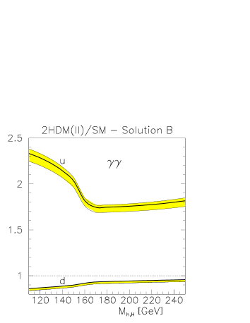
Figure 4: The ratio of the two–photon Higgs width in the 2HDM to its SM value, for two different solutions [87, 88].

The ${\cal CP}$ parity of the neutral Higgs boson can be measured using linearly polarised photons. Moreover, if the Higgs boson is a mixture of ${\cal CP}$–even and ${\cal CP}$–odd states, for instance in a general 2HDM with a ${\cal CP}$–violating neutral sector, the interference of these two terms gives rise to a ${\cal CP}$–violating asymmetry [43, 44, 45, 84, 89]. Two ${\cal CP}$–violating ratios could be observed to linear order in the ${\cal CP}$–violating couplings:

$${\mathcal{A}_{1}}=\frac{|{\mathcal{M}}_{++}|^{2}-|{\mathcal{M}}_{--}|^{2}}{|{\mathcal{M}}_{++}|^{2}+|{\mathcal{M}}_{--}|^{2}},\quad{\mathcal{A}}_{2}=\frac{2\Im({\mathcal{M}}_{--}^{*}{\mathcal{M}}_{++})}{|{\mathcal{M}}_{++}|^{2}+|{\mathcal{M}}_{--}|^{2}}.$$

In terms of experimental values the first asymmetry can be found from

$$T_{-}=\frac{N_{++}-N_{--}}{N_{++}+N_{--}}=\frac{\langle\xi_{2}\rangle+\langle\tilde{\xi}_{2}\rangle}{1+\langle\xi_{2}\tilde{\xi}_{2}\rangle}{\mathcal{A}}_{1},$$

where $N_{\pm\pm}$ correspond to the event rates for positive (negative) initial photon helicities and $\xi_{i}$, $\tilde{\xi}_{i}$ are the Stokes polarisation parameters. The measurement of the asymmetry is achieved by simultaneously flipping the helicities of the laser beams used for production of polarised electrons and $\gamma\to e$ conversion. The asymmetry to be measured with linearly polarised photons is given by

$$T_{\psi}=\frac{N(\phi=\frac{\pi}{4})-N(\phi=-\frac{\pi}{4})}{N(\phi=\frac{\pi}{4})+N(\phi=-\frac{\pi}{4})}=\frac{\langle\xi_{3}\tilde{\xi}_{1}\rangle+\langle\xi_{1}\tilde{\xi}_{3}\rangle}{1+\langle\xi_{2}\tilde{\xi}_{2}\rangle}{\mathcal{A}}_{2},$$ (4)

where $\phi$ is the angle between the linear polarisation vectors of the photons. The asymmetries are typically larger than 10% and they are observable for a large range of the 2HDM parameter space if ${\cal CP}$ violation is present in the Higgs potential.

Hence, high degrees of both circular and linear polarisations for the high energy photon beams provide additional analysing power for the detailed study of the Higgs sector at the $\gamma\gamma$ collider.

3 Supersymmetry

In $\gamma\gamma$ collisions, any kind of charged particle can be produced in pairs, provided the mass is below the kinematical bound. Potential SUSY targets for a photon collider are the charged sfermions [18, 90], the charginos [18, 91] and the charged Higgs bosons.

For the $\gamma\gamma$ luminosity given in the Table 1, the production rates for these particles will be larger than that in $e^{+}e^{-}$ collisions and detailed studies of the charged supersymmetric particles should be possible. In addition, the cross sections in $\gamma\gamma$ collisions are given just by QED to leading order, while in $e^{+}e^{-}$ collisions also $Z$ boson and (sometimes) t–channel exchanges contribute. So, studying these processes in both channels provides complementary information about the interactions of the charged supersymmetric particles.

The $\gamma e$ collider could be the ideal machine for the discovery of scalar electrons ($\tilde{e}$) and neutrinos ($\tilde{\nu}$) in the reactions $\gamma e\to\tilde{e}^{-}\tilde{\chi}_{1}^{0},\,\tilde{W}\tilde{\nu}$ [18, 92, 93, 94, 95, 96]. Selectrons and neutralinos may be discovered in $\gamma e$ collisions up to the kinematical limit of

$$M_{{\tilde{e}^{-}}}<0.9\times 2E_{0}-M_{{\tilde{\chi}_{i}^{0}}},$$ (5)

where $2E_{0}$ is the energy of the original $e^{+}e^{-}$ collider. This bound is larger than the bound obtained from $\tilde{e}^{+}\tilde{e}^{-}$ pair production in the $e^{+}e^{-}$ mode, if $M_{{\tilde{\chi}_{i}^{0}}}<0.4\times 2E_{0}$.

In Fig. 5 the cross section of the process $\gamma e\rightarrow\tilde{\chi}_{1}^{0}\tilde{e}_{L/R}^{-}\rightarrow\tilde{\chi}_{1}^{0}\tilde{\chi}_{1}^{0}e^{-}$ is compared to the cross section of the process $e^{+}e^{-}\rightarrow\tilde{e}_{L/R}^{+}\tilde{e}^{-}_{L/R}\rightarrow\tilde{\chi}_{1}^{0}\tilde{\chi}_{1}^{0}e^{+}e^{-}$ for the MSSM parameters $M_{2}=152\,\mathrm{GeV}$, $\mu=316\,\mathrm{GeV}$, $\tan\beta=3$ and $M_{{\tilde{e}_{R}}}=260\,\mathrm{GeV}$, $M_{{\tilde{e}_{L}}}=290\,\mathrm{GeV}$ (Fig. 5a) and $M_{{\tilde{e}_{R}}}=230\,\mathrm{GeV}$, $M_{{\tilde{e}_{L}}}=270\,\mathrm{GeV}$ (Fig. 5b) [97, 98]. The $\tilde{\chi}_{1}^{0}$ mass in this case is about $70\,\mathrm{GeV}$. For higher selectron masses pair production in $e^{+}e^{-}$ annihilation at $2E_{0}=500\,\mathrm{GeV}$ is kinematically forbidden, whereas in $\gamma e$ collisions the cross section at $2E_{0}=500\,\mathrm{GeV}$ is $96\,\mathrm{fb}$. According to (5) the highest accessible selectron mass for $2E_{0}=500\,\mathrm{GeV}$ is $M_{{\tilde{e}}}<380\,\mathrm{GeV}$ in this scenario.

Figure 5: Total cross sections for $\gamma e\rightarrow\tilde{\chi}_{1}^{0}\tilde{e}_{L/R}^{-}\rightarrow\tilde{\chi}_{1}^{0}\tilde{\chi}_{1}^{0}e^{-}$ (solid curves) for longitudinal polarisation $P_{e^{-}}=0.8$ and longitudinal (circular) polarisation $P_{e_{c}}=0.8$ ($\lambda_{L}=-1$) of the converted electrons (laser photons) compared to $e^{+}e^{-}\rightarrow\tilde{e}_{L/R}^{+}\tilde{e}^{-}_{L/R}\rightarrow\tilde{\chi}_{1}^{0}\tilde{\chi}_{1}^{0}e^{+}e^{-}$ (dashed curves) with longitudinally polarised electrons, $P_{e^{-}}=0.8$, and unpolarised positrons. MSSM parameters: $M_{2}=152\,{GeV}$, $\mu=316\,{GeV}$, $\tan\beta=3$. (a) $M_{{\tilde{e}_{R}}}=260\,{GeV}$, $M_{{\tilde{e}_{L}}}=290\,{GeV}$. (b) $M_{{\tilde{e}_{R}}}=230\,{GeV}$, $M_{{\tilde{e}_{L}}}=270\,{GeV}$.

In some scenarios of supersymmetric extensions of the Standard Model the stoponium bound states $\tilde{t}\bar{\tilde{t}}$ is formed. A photon collider would be the ideal machine for the discovery and study of these new narrow strong resonances [99]. About ten thousand stoponium resonances for $M_{S}=200\,\mathrm{GeV}$ will be produced for an integrated luminosity in the high energy peak of $100\,\mathrm{fb}^{-1}$. Thus precise measurements of the stoponium effective couplings, mass and width should be possible. At $e^{+}e^{-}$ colliders the counting rate will be much lower and in some scenarios the stoponium cannot be detected due to the large background [99].

4 Extra dimensions

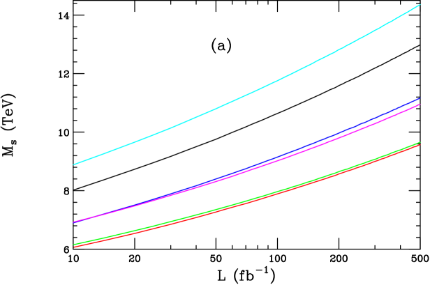
Figure 6: $M_{s}$ discovery reach for the process $\gamma\gamma\to W^{+}W^{-}$ at a $2E_{0}=1\,{TeV}$ LC as a function of the integrated luminosity for the different initial state polarizations assuming $\lambda=1$. From top to bottom on the right hand side of the figure the polarisations are $(-++-)$, $(+---)$, $(++--)$, $(+-+-)$, $(+---)$, and $(++++)$.

New ideas have recently been proposed to explain the weakness of the gravitational force [100, 101, 102]. The Minkowski world is extended by extra space dimensions which are curled up at small dimensions $R$. While the gauge and matter fields are confined in the (3+1) dimensional world, gravity propagates through the extended 4+n dimensional world. While the effective gravity scale, the Planck scale, in four dimensions is very large, the fundamental Planck scale in 4+n dimensions may be as low as a few TeV so that gravity may become strong already at energies of the present or next generation of colliders.

Towers of Kaluza–Klein graviton excitations will be realised on the compactified 4+n dimensional space. Exchanging these KK excitations between SM particles in high–energy scattering experiments will generate effective contact interactions, carrying spin=2 and characterised by a scale $M_{s}$ of order few TeV. They will give rise to substantial deviations from the predictions of the Standard Model for the cross sections and angular distributions for various beam polarisations [103, 104, 105, 106, 107, 108].

Of the many processes examined so far, $\gamma\gamma\to WW$ provides the largest reach for $M_{s}$ for a given centre of mass energy of the LC [109, 108]. The main reasons are that the $WW$ final state offers many observables which are particularly sensitive to the initial electron and laser polarisations and the very high statistics due to the $80\,\mathrm{pb}$ cross section.

By performing a combined fit to the total cross sections and angular distributions for various initial state polarisation choices and the polarisation asymmetries, the discovery reach for $M_{s}$ can be estimated as a function of the total $\gamma\gamma$ integrated luminosity. This is shown in Fig. 6 [108]. The reach is in the range of $M_{s}\sim(11$–$13)\cdot 2E_{0}$, which is larger than that obtained from all other processes examined so far. By comparison, a combined analysis of the processes $e^{+}e^{-}\to f\bar{f}$ with the same integrated luminosity leads to a reach of only $(6$–$7)\cdot 2E_{0}$.

Other $\gamma\gamma$ final states are also sensitive to graviton exchanges, two examples being the $\gamma\gamma$ [110, 111] and $ZZ$ [109] final states, which however result in smaller search reaches.

5 Gauge bosons

New strong interactions that might be responsible for the electroweak symmetry breaking can affect the triple and quartic couplings of the weak vector bosons. Hence, the precision measurements of these couplings, as well as corresponding effects on the top quark couplings, can provide clues to the mechanism of the electroweak symmetry breaking.

Due to the large cross sections of the order of $10^{2}\,\mathrm{pb}$ well above the thresholds, the $\gamma\gamma\to W^{+}W^{-}$ and $\gamma e\to\nu W$ processes seem to be ideal reactions to study such anomalous gauge interactions [112, 113].

Anomalous gauge boson couplings

The relevant process at the $e^{+}e^{-}$ collider is $e^{+}e^{-}\to W^{+}W^{-}$. This reaction is dominated by the large t–channel neutrino exchange term which however can be suppressed using electron beam polarisation. The cross section of $W^{+}W^{-}$ pair production in $e^{+}e^{-}$ collisions with right–handed electron beams, for which the neutrino exchange is negligible, has a maximum of about $2\,\mathrm{pb}$ at LEP2 and decreases at higher energy.

The two main processes at the Photon Collider are $\gamma\gamma\to W^{+}W^{-}$ and $\gamma e\to W\nu$. Their total cross sections for centre–of–mass energies above $200\,\mathrm{GeV}$ are about $80\,\mathrm{pb}$ and $40\,\mathrm{pb}$, respectively, and they do not decrease with energy. Hence the $W$ production cross sections at the Photon Collider are at least $20$–$40$ times larger than the cross section at the $e^{+}e^{-}$ collider. This enhancement makes event rates at the Photon Collider one order of magnitude larger than at an $e^{+}e^{-}$ collider, even when the lower $\gamma\gamma$, $\gamma e$ luminosities are taken into account. Specifically for the integrated $\gamma\gamma$ luminosity of $100\,\mathrm{fb}^{-1}$, about $8\times 10^{6}$ $W^{+}W^{-}$ pairs are produced at the Photon Collider. Note that while $\gamma e\to W\nu$ and $\gamma\gamma\to WW$ isolate the anomalous photon couplings to the $W$, $e^{+}e^{-}\to WW$ involves potentially anomalous $Z$ couplings so that the two LC modes are complementary with each other.

The analysis of $\gamma\gamma\ \to WW$ has been performed in [18, 114] with the detector simulation. The $W$ boson by photon colliders is compared to that from $e^{+}e^{-}$ colliders. The results have been obtained only from analyses of the total cross section. With the $W$ decay properties taken into account further improvements can be expected. The resulting accuracy on $\lambda_{\gamma}$ is comparable with $e^{+}e^{-}$ analyses, while a similar accuracy on $\delta\kappa_{\gamma}$ can be achieved at $1/20$–th of the $e^{+}e^{-}$ luminosity. In addition, the process $\gamma e\to W\nu$, which has a large cross section, is very sensitive to the admixture of right–handed currents in the $W$ couplings with fermions: $\sigma_{\gamma e\to W\nu}\propto(1$–$2\lambda_{e})$.

Many processes of 3rd and 4th order have quite large cross sections [115, 116, 117, 118] at the Photon Collider:

$\gamma e\to eWW$

$\gamma e\to\nu WZ$

$\gamma\gamma\to ZWW$

$\gamma\gamma\to WWWW$

$\gamma\gamma\to WWZZ$

It should also be noted, that in $\gamma\gamma$ collisions the anomalous $\gamma\gamma W^{+}W^{-}$ quartic couplings can be probed. However, the higher event rate does not necessarily provide better bounds on anomalous couplings. In some models electroweak symmetry breaking leads to large deviations mainly in longitudinal $W_{L}W_{L}$ pair production [119]. On the other hand the large cross section of the reaction $\gamma\gamma\to W^{+}W^{-}$ is due to transverse $W_{T}W_{T}$ pair production. In such a case transverse $W_{T}W_{T}$ pair production would represent a background for the longitudinal $W_{L}W_{L}$ production. The relative yield of $W_{L}W_{L}$ can be considerably improved after a cut on the $W$ scattering angle. Asymptotically for $s_{\gamma\gamma}\gg M_{W}^{2}$ the production of $W_{L}W_{L}$ is as much as 5 times larger than at a $e^{+}e^{-}$ LC.

However, if anomalous couplings manifest themselves in transverse $W_{T}W_{T}$ pair production, e.g. in theories with large extra dimensions, then the interference with the large SM transverse contribution is of big advantage in the Photon Collider.

Strong WW $\bto$ WW, WW $\bto$ ZZ scattering

If the strong electroweak symmetry breaking scenario is realised in Nature, $W$ and $Z$ bosons will interact strongly at high energies. If no Higgs boson exists with a mass below $1\,\mathrm{TeV}$, the longitudinal components of the electroweak gauge bosons must become strongly interacting at energies above $1\,\mathrm{TeV}$. In such scenarios novel resonances can be formed in $W_{L}W_{L}$ collisions at energies $\raisebox{-1.9919pt}{$\,\stackrel{{\scriptstyle<}}{{{\scriptstyle\sim}}}\,$}3\,\mathrm{TeV}$. If the energy of the $\gamma\gamma$ collisions is sufficiently high, the effective $W$ luminosities in $\gamma\gamma$ collisions allow the study of $W^{+}W^{-}\to W^{+}W^{-}$, $ZZ$ scattering in the reactions

$$\gamma\gamma\to WWWW,\;\;WWZZ$$

for energies in the threshold region of the new strong interactions. Each incoming photon turns into a virtual $WW$ pair, followed by the scattering of one $W$ from each such pair to form $WW$ or $ZZ$ [120, 121, 122, 123, 124, 125, 126]. The same reactions can be used to study quartic anomalous $WWWW$, $WWZZ$ couplings.

6 Top quark

The top quark is heavy and up to now point–like at the same time. The top Yukawa coupling $\lambda_{t}=2^{3/4}G_{F}^{1/2}M_{t}$ is numerically very close to unity, and it is not clear whether or not this is related to a deep physics reason. Hence one might expect deviations from SM predictions to be most pronounced in the top sector [127, 128]. Besides, top quarks decay before forming a bound state with any other quark. Top quark physics will be a very important part of research programs for all future hadron and lepton colliders. The $\gamma\gamma$ collider is of special interest because of the clean production mechanism and the high rate (review [129]). Moreover, the $S$ and $P$ partial waves of the final state top quark–antiquark pair produced in $\gamma\gamma$ collisions can be separated by choosing the same or opposite helicities of the colliding photons.

Probe for anomalous couplings in t$\bbar{\rm\bf t}$ pair production

There is a difference for the case of $\gamma\gamma$ and $e^{+}e^{-}$collisions with respect to the couplings: the $\gamma t\bar{t}$ coupling is separated from $Zt\bar{t}$ coupling in $\gamma\gamma$ collisions while in $e^{+}e^{-}$ collisions both couplings contribute.

The effective Lagrangian contains four parameters $f_{i}^{\alpha}$ for the electric and magnetic type couplings [130], where $i=1$–$4$ and $\alpha=\gamma,Z$ but only couplings with $\alpha=\gamma$ occur in $\gamma\gamma$ collisions. It was demonstrated [131] that if the cross section can be measured with 2% accuracy, scale parameter for new physics $\Lambda$ up to $10\,\mathrm{TeV}$ for $2E_{0}=500\,\mathrm{GeV}$ can be probed for form factors taken in the form $f_{i}^{\alpha}=(f_{i}^{\alpha})^{SM}(1+s/\Lambda^{2})$. The sensitivity to the anomalous magnetic moment $f_{2}^{\gamma}$ is of similar size in $\gamma\gamma$ and $e^{+}e^{-}$ collisions. The $f_{4}^{\alpha}$ term describes the ${\cal CP}$ violation. The best limit on the imaginary part of the electric dipole moment $\Im(f_{4}^{\gamma})\sim 2.3\times 10^{-17}e\,\mathrm{cm}$ [132] by measuring the forward–backward asymmetry $A_{fb}$ with initial–beam helicities of electron and laser beams $\lambda_{e}^{1}=\lambda_{e}^{2}$ and $\lambda_{l}^{1}=-\lambda_{l}^{2}$. The achievable limit for the real part of the dipole moment is also of the order of $10^{-17}e\,\mathrm{cm}$ and is obtained from the linear polarisation asymmetries [133, 134].

Figure 7: Single top quark production cross section in $\gamma e$ collisions as a function of $2E_{0}$.

Single top production in $\bgamma\bgamma$ and $\bgamma$e Collisions

Single top production in $\gamma\gamma$ collisions results in the same final state as top quark pair production [135] and invariant mass cuts are required to suppress direct $t\bar{t}$ contributions. Single top production is preferentially realised in $\gamma e$ collisions [136, 137, 138, 139, 140]. In contrast to the top pair production rate, the single top rate is directly proportional to the $Wtb$ coupling and the process is very sensitive to its structure. The anomalous part of the effective Lagrangian [130] contains terms $f_{2L(R)}\propto 1/\Lambda$, where $\Lambda$ is the scale of a new physics.

	$f_{2L}$	$f_{2R}$
TEVATRON ($\Delta_{sys.}\approx 10\%$)	$-0.18\div+0.55$	$-0.24\div+0.25$
LHC ($\Delta_{sys.}\approx 5\%$)	$-0.052\div+0.097$	$-0.12\div+0.13$
$e^{+}e^{-}$ ($2E_{0}=0.5\,\mathrm{TeV}$)	$-0.025\div+0.025$	$-0.2\div+0.2$
$\gamma e$ ($2E_{0}=0.5\,\mathrm{TeV}$)	$-0.045\div+0.045$	$-0.045$ $\div+0.045$
$\gamma e$ ($2E_{0}=2.0\,\mathrm{TeV}$)	$-0.008\div+0.035$	$-0.016\div+0.016$

Table 1: Expected sensitivity for the $Wtb$ anomalous couplings. The total integrated luminosity was assumed to be $500fb^{-1}$ for $e^{+}e^{-}$ collisions and $250fb^{-1}$ and $500~{}fb^{-1}$ for $\gamma e$ collisions at $500\,{GeV}$ and $2\,{TeV}$, respectively.

In Table 1 [141, 142] limits on anomalous couplings from measurements at different accelerators are collected. The best limits can be reached at very high energy $\gamma e$ colliders, even in the case of unpolarised collisions. In the case of polarised collisions, the production rate increases significantly as shown in Fig. 7 [135] and more stringent bounds on anomalous couplings may be achieved.

7 QCD and hadron physics

Photon colliders offer a unique possibility to probe QCD in a new unexplored regime. The very high luminosity, the (relatively) sharp spectrum of the backscattered laser photons and their polarisation are of great advantage. At the Photon Collider the following measurements can be performed, for example:

1. The total cross section for $\gamma\gamma$ fusion to hadrons [143].

2. Deep inelastic $\gamma e$ ${\cal NC}$ and ${\cal CC}$ scattering, and measurement of the quark distributions in the photon at large $Q^{2}$.

3. Measurement of the gluon distribution in the photon.

4. Measurement of the spin dependent structure function $g_{1}^{\gamma}(x,Q^{2})$ of the photon.

5. $J/\Psi$ production in $\gamma\gamma$ collisions as a probe of the hard QCD pomeron [144, 145, 146].

$\bgamma\bgamma$ fusion to hadrons

The total cross section for hadron production in $\gamma\gamma$ collisions is a fundamental observable. It provides us with a picture of hadronic fluctuations in photons of high energy which reflect the strong–interaction dynamics as described by quarks and gluons in QCD. Since these dynamical processes involve large distances, predictions, due to the theoretical complexity, cannot be based yet on first principles. Instead, phenomenological models have been developed which involve elements of ideas which have successfully been applied to the analysis of hadron–hadron scattering, but also elements transferred from perturbative QCD in eikonalised mini–jet models. Differences between hadron–type models and mini–jet models are dramatic in the TESLA energy range. $\gamma\gamma$ scattering experiments are therefore extremely valuable in clarifying the dynamics in complex hadronic quantum fluctuations of the simplest gauge particle in Nature.

Deep inelastic $\bgamma$e scattering (DIS)

The large c.m. energy in the $\gamma e$ system and the possibility of precise measurement of the kinematical variables $x,Q^{2}$ in DIS provide exciting opportunities at a photon collider. In particular it allows precise measurements of the photon structure function(s) with much better accuracy than in the single tagged $e^{+}e^{-}$ collisions. The $\gamma e$ collider offers a unique opportunity to probe the photon at low values of $x$ ($x\sim 10^{-4}$) for reasonably large values of $Q^{2}\sim 10\,\mathrm{GeV}^{2}$ [147]. At very large values of $Q^{2}$ the virtual $\gamma$ exchange in deep inelastic $\gamma e$ scattering is supplemented by significant contributions from $Z$ exchange. Moreover, at very large values of $Q^{2}$ charged–current exchange becomes effective in deep inelastic scattering, $\gamma e\to\nu X$, which is mediated by virtual $W$ exchange. The study of this process can in particular give information on the flavour decomposition of the quark distributions in the photon [148].

Gluon distribution in the photon

The gluon distribution in the photon can be studied in dedicated measurements of the hadronic final state in $\gamma\gamma$ collisions. The following two processes are of particular interest:

1. Dijet production [149, 150], generated by the subprocess $\gamma g\to q\bar{q}$.

2. Charm production [151], which is sensitive to the mechanism $\gamma g\to c\bar{c}$

Both these processes, which are at least in certain kinematical regions dominated by the photon–gluon fusion mechanisms, are sensitive to the gluon distribution in the photon. The detailed discussion of these processes have been presented in [152, 153].

Measurement of the spin dependent structure function g${}_{\bone}^{\bgamma}$(x,Q${}^{\btwo}$) of the Photon

Using polarised beams, photon colliders offer the possibility to measure the spin dependent structure function $g_{1}^{\gamma}(x,Q^{2})$ of the photon [154, 155, 156]. This quantity is completely unknown and its measurement in polarised $\gamma e$ DIS would be extremely interesting for testing QCD predictions in a broad region of $x$ and $Q^{2}$. The high–energy photon colliders allow to probe this quantity for very small values of $x$ [157, 158].

Probing the QCD pomeron by J/$\bPsi$ production in $\bgamma\bgamma$ Collisions

The exchange of the hard QCD (or BFKL) pomeron is presumably the dominant mechanism of the process $\gamma\gamma\to J/\psi\,J/\psi$. Theoretical estimates of the cross–section presented in [159, 160] have demonstrated that measurement of the reaction $\gamma\gamma\to J/\psi\,J/\psi$ at the Photon Collider should be feasible.

8 Table of gold–plated processes

A short list of processes which we think are the most important ones for the physics program of the Photon Collider option of the LC is presented in Table 2.

Reaction	Remarks
$\gamma\gamma\to h^{0}\to b\bar{b}$	SM (or MSSM ) Higgs, $M_{h^{0}}<160\,\mathrm{GeV}$
$\gamma\gamma\to h^{0}\to WW(WW^{*})$	SM Higgs, $140\,\mathrm{GeV}<M_{h^{0}}<190\,\mathrm{GeV}$
$\gamma\gamma\to h^{0}\to ZZ(ZZ^{*})$	SM Higgs, $180\,\mathrm{GeV}<M_{h^{0}}<350\,\mathrm{GeV}$
$\gamma\gamma\to H,A\to b\bar{b}$	MSSM heavy Higgs, for intermediate $\tan\beta$
$\gamma\gamma\to\tilde{f}\bar{\tilde{f}},\ \tilde{\chi}^{+}_{i}\tilde{\chi}^{-}_{i},\ H^{+}H^{-}$	large cross sections, possible observations of FCNC
$\gamma\gamma\to S[\tilde{t}\bar{\tilde{t}}]$	$\tilde{t}\bar{\tilde{t}}$ stoponium
$\gamma e\to\tilde{e}^{-}\tilde{\chi}_{1}^{0}$	$M_{{\tilde{e}^{-}}}<0.9\times 2E_{0}-M_{{\tilde{\chi}_{1}^{0}}}$
$\gamma\gamma\to W^{+}W^{-}$	anomalous $W$ interactions, extra dimensions
$\gamma e^{-}\to W^{-}\nu_{e}$	anomalous $W$ couplings
$\gamma\gamma\to WWWW$,$WWZZ$	strong $WW$ scatt., quartic anomalous $W$, $Z$ couplings
$\gamma\gamma\to t\bar{t}$	anomalous top quark interactions
$\gamma e^{-}\to\bar{t}b\nu_{e}$	anomalous $Wtb$ coupling
$\gamma\gamma\to$ hadrons	total $\gamma\gamma$ cross section
$\gamma e^{-}\to e^{-}X$ and $\nu_{e}X$	${\cal NC}$ and ${\cal CC}$ structure functions (polarised and unpolarised)
$\gamma g\to q\bar{q},\ c\bar{c}$	gluon distribution in the photon
$\gamma\gamma\to J/\psi\,J/\psi$	QCD Pomeron

Table 2: Gold–plated processes at photon colliders

Of course there exist many other possible manifestations of new physics in $\gamma\gamma$ and $\gamma e$ collisions which we have not discussed here. The study of resonant production of excited electrons $\gamma e\to e^{*}$, the production of excited fermions $\gamma\gamma\to f^{*}f$, leptoquark production $\gamma e\to(eQ)\bar{Q}$ [161, 162], a magnetic monopole signal in the reaction of $\gamma\gamma$ elastic scattering [163, 164] etc. may be mentioned in this context.

To summarise, the Photon Collider will allow us to study the physics of the EWSB in both the weak–coupling and the strong–coupling scenarios. Measurements of the two–photon Higgs width of the $h$, $H$ and $A$ Higgs states provide a strong physics motivation for developing the technology of the $\gamma\gamma$ collider option. Polarised photon beams, large cross sections and sufficiently large luminosities allow to significantly enhance the discovery limits of many new particles in SUSY and other extensions of the Standard Model. Moreover, they will substantially improve the accuracy of the precision measurements of anomalous $W$ boson and top quark couplings, thereby complementing and improving the measurements at the $e^{+}e^{-}$ mode of TESLA. Photon colliders offer a unique possibility for probing the photon structure and the QCD Pomeron.

3 Electron to Photon Conversion

1 Processes in the conversion region

Compton scattering

Compton scattering is the basic process for the production of high energy photons at photon colliders. The fact that a high energy electron loses a large fraction of its energy in collisions with an optical photon was realized a long time ago in astrophysics [165]. The method of generation of high energy $\gamma$–quanta by Compton scattering of the laser light on relativistic electrons has been proposed soon after lasers were invented [166, 167] and has already been used in many laboratories for more than 35 years [168, 169]. In first experiments the conversion efficiency of electron to photons $k=N_{\gamma}/N_{e}$ was very small, only about $10^{-7}$ [169]. At linear colliders, due to small bunch sizes one can focus the laser to the electron beam and get $k\approx 1$ at rather moderate laser flash energy, about $1$–$5\,\mathrm{J}$. Twenty years ago when photon colliders were proposed [1, 2] such flash energies could already be obtained but with a low rate and a pulse duration longer than is necessary. Progress in laser technology since that time now presents a real possibility for the construction of a laser system for a photon collider.

Kinematics, photon spectrum

Let us consider the most important characteristics of Compton scattering. In the conversion region a laser photon with energy $\omega_{0}$ scatters at a small collision angle $\alpha_{0}$ off a high energy electron with energy $E_{0}$. The energy of the scattered photon $\omega$ depends on the photon scattering angle as follows [2]:

$$\omega=\frac{\omega_{m}}{1+(\vartheta/\vartheta_{0})^{2}},\;\;\;\;\omega_{m}=\frac{x}{x+1}E_{0},\;\;\;\;\vartheta_{0}=\frac{mc^{2}}{E_{0}}\sqrt{x+1},$$ (1)

where

$$x=\frac{4E_{0}\omega_{0}}{m^{2}c^{4}}cos^{2}{\alpha_{0}/2}\simeq 15.3\left[\frac{E_{0}}{\,\mathrm{TeV}}\right]\left[\frac{\omega_{0}}{\,\mathrm{eV}}\right]=19\left[\frac{E_{0}}{\,\mathrm{TeV}}\right]\left[\frac{\mu m}{\lambda}\right],$$ (2)

$\omega_{m}$ is the maximum energy of scattered photons (in the direction of the electron, Compton “backscattering”).

For example: $E_{0}=250\,\mathrm{GeV}$, $\omega_{0}=1.17\,\mathrm{eV}$ ($\lambda=1.06\,\mu\mathrm{m}$) (region of most powerful solid–state lasers) $\Rightarrow x=4.5$ and $\omega_{m}/E_{0}=0.82$.

The energy spectrum of the scattered photons is defined by the Compton cross section

$$\frac{1}{\sigma_{c}}{d\sigma_{c}\over dy}={2\sigma_{0}\over x\sigma_{c}}\left[{1\over 1-y}+1-y-4r(1-r)+2\lambda_{e}P_{c}rx(1-2r)(2-y)\right]\,,$$ (3)

$$y=\omega/E_{0},\;\;\;\;\;r=\frac{y}{(1-y)x},\;\;\;\sigma_{0}=\pi r_{e}^{2}=\pi\left({e^{2}\over mc^{2}}\right)^{2}=2.5\cdot 10^{-25}\,\mathrm{cm}^{2}\,,$$

where $\lambda_{e}$ is the mean electron helicity ($|\lambda_{e}|\leq 1/2$) and $P_{c}$ is that of the laser photon ($|P_{c}|\leq 1$). It is useful to note that $r\to 1$ for $y\to y_{m}$.

The total Compton cross section is

$$\sigma_{c}\;=\;\sigma_{c}^{0}\;+\;2\lambda_{e}P_{c}\,\sigma_{c}^{1}\,,$$

$$\sigma_{c}^{0}\;=\;{2\sigma_{0}\over x}\left[\left(1-{4\over x}-{8\over x^{2}}\right)\ln(x+1)+{1\over 2}+{8\over x}-{1\over 2(x+1)^{2}}\right]\,,$$ (4)

$$\sigma_{c}^{1}\;=\;{2\sigma_{0}\over x}\left[\left(1+{2\over x}\right)\ln(x+1)-{5\over 2}+{1\over x+1}-{1\over 2(x+1)^{2}}\right]\,.$$

Polarisations of initial beams influence the differential and the total cross section only if both their helicities are nonzero, i.e. at $\lambda_{e}P_{c}\neq 0$. In the region of interest

$$x=1\div 5,\;\;\;\sigma_{c}^{0}=(1.5\div 0.7)\,\sigma_{0}\,,\;\;\;|\sigma_{c}^{1}|/\sigma_{c}<0.1\,,$$ (5)

i.e. the total cross section only depends slightly on the polarisation.

On the contrary, the energy spectrum strongly depends on the value of $\lambda_{e}P_{c}$. The “quality” of the photon beam, i.e. the relative number of hard photons, is improved when one uses beams with a negative value of $\lambda_{e}P_{c}$. For $2\lambda_{e}P_{c}=-1$ the peak at $\omega=\omega_{m}$ nearly doubles, significantly improving the energy spread of the $\gamma$ beam

$${d\sigma_{c}(y_{m},2\lambda_{e}P_{c}=-1)/dy\over d\sigma_{c}(y_{m},2\lambda_{e}P_{c}=0)/dy}={2\over 1+(x+1)^{-2}}\,.$$

The full width of the spectrum at the half of maximum is $\Delta\omega_{1/2}\approx\omega_{m}/(x+2)$ for unpolarised beams, and even smaller at $\lambda_{e}P_{c}<0$. Photons in this high energy peak have the characteristic angle $\theta_{{\rm char}}=1/\gamma=mc^{2}/E=0.51/E_{0}[\,\mathrm{TeV}]\;\mu\mbox{rad}$.

To increase the maximum photon energy, one should use a laser with a higher energy. This also increases the fraction of hard photons. Unfortunately, at large $x>4.8$, a new phenomenon takes place: the high energy photons disappear from the beam, producing $e^{+}e^{-}$ pairs in collisions with laser photons (see Section 1). Therefore, the value $x\approx 4.8$ is the most preferable.

The energy spectrum of the scattered photons for $x=4.8$ is shown in Fig. 1 for various helicities of electron and laser beams. As was mentioned before, with the polarised beams at $2\lambda_{e}P_{c}=-1$, that the number of high energy photons nearly doubles and the luminosity in collisions of these photons is larger by a factor of 4. This is one of the important advantages of polarised electron beams.

The photon energy spectrum presented in Fig. 1 corresponds to the case of a small conversion coefficient. In the realistic case when the thickness of the laser target is about one collision length each electron may undergo multiple Compton scattering [5]. This probability is not small because, after a large energy loss in the first collision, the Compton cross section increases and approaches the Thomson cross section $\sigma_{T}=(8/3)\sigma_{0}$. The secondary photons are softer and populate the low energy part of the spectrum. Multiple Compton scattering leads also to a low energy tail in the energy spectrum of the electron beam after the $e\to\gamma$ conversion. This creates a problem for the removal of the beams (see Section 2).

Figure 1: Spectrum of the Compton scattered photons for different polarisations of the laser and electron beams.

Polarisation of scattered photons

The averaged helicity of photons after Compton scattering is [3]

$$\langle\lambda_{\gamma}\rangle={-P_{c}(2r-1)[(1-y)^{-1}+1-y]+2\lambda_{e}xr[1+(1-y)(2r-1)^{2}]\over(1-y)^{-1}+1-y-4r(1-r)-2\lambda_{e}P_{c}xr(2-y)(2r-1)}\;.$$ (6)

The final photons have an averaged helicity $\langle\lambda_{\gamma}\rangle\neq 0$ if either the laser light has circular polarisation $P_{c}\neq 0$ or the electrons have mean helicity $\lambda_{e}\neq 0$. Moreover, $\langle\lambda_{\gamma}(\omega=\omega_{m})\rangle=-P_{c}$ at $P_{c}=\pm 1$ or $\lambda_{e}=0$.

Figure 2: Mean helicity of the scattered photons.

Figure 3: Mean helicity of the scattered photons for various $x$ and degree of the longitudinal electron polarisation.

The mean helicity of the scattered photons at $x=4.8$ is shown in Fig. 2 for various helicities of the electron and laser beams [5]. For $2P_{c}\lambda_{e}=-1$ (the case with minimum energy spread) all photons in the high energy peak have a high degree of like–sign polarisation. This is the most valuable region for experiments. If the electron polarisation is not 100% and $|P_{c}|=1$, the helicity of the photon with the maximum energy is still 100% but the energy region with a high helicity is reduced, see 3.

Low energy photons are also polarised (especially in the case $2\lambda_{e}P_{c}=+1$ which corresponds to the broad spectrum), but due to contribution of multiple Compton scattering and beamstrahlung photons produced during the beam collisions the low energy region is not attractive for polarisation experiments.

A high degree of longitudinal photon polarisation is essential for the suppression of the QED background in the study of the intermediate Higgs boson (Section 2). Note that at a $0.5\,\mathrm{TeV}$ linear collider the region of the intermediate Higgs can be studied with rather small $x$. In this case the helicity of scattered photons is almost independent of the polarisation of the electrons, and, if $P_{c}=1$, the high energy photons have very high circular polarisation over a wide range near the maximum energy, even with $\lambda_{e}=0$. Nevertheless, electron polarisation is very desirable even for rather low $x$ because, as was mentioned before, it increases the relative number of high energy photons.

Figure 4: Linear polarisation of the scattered photons for various $x$ for unpolarised electrons and $P_{l}=1$.

The averaged degree of the linear polarisation of the final photons is [3]

$$\langle l_{\gamma}\rangle={2r^{2}\;P_{l}\over(1-y)^{-1}+1-y-4r(1-r)-2\lambda_{e}P_{c}xr(2-y)(2r-1)}\,.$$ (7)

If the laser light has a linear polarisation, then the high-energy photons are polarised in the same direction. The degree of this polarisation $\langle l_{\gamma}\rangle$ depends on the linear polarisation of laser photons $P_{l}$ and $2\lambda_{e}\,P_{c}$. For $P_{l}=1$ (in this case $P_{c}=0$) the linear polarisation is maximum for the photons with the maximum energy. At $y=y_{m}$ the degree of linear polarisation for the unpolarised electrons

$$l_{\gamma}=\frac{2}{1+x+(1+x)^{-1}}$$ (8)

is 0.334, 0.6, 0.8 for $x=4.8,2,1$ respectively. The dependence of the linear polarisation on the photon energy for unpolarised electron beams and 100% linear polarisation of laser photons is shown in Fig. 4

It is of interest that varying polarisations of laser and electron beams one can get larger $\langle l_{\gamma}\rangle$, up to $\langle l_{\gamma}\rangle=1$. For example, at $P_{t}=2(x+1)/(x^{2}+2x+2)$ and $2\lambda_{e}\,P_{c}=x(x+2)/(x^{2}+2x+2)$ the quantity $\langle l_{\gamma}\rangle$ at $y=y_{m}$ can reach 1. Unfortunately, in this case $2\lambda_{e}\,P_{c}\approx+1$, which corresponds to curve $c$ in Fig. 1, when the number of photons with the energy $\omega$ near $\omega_{m}$ is small.

Linear polarisation is necessary for the measurement of the ${\cal CP}$–parity of the Higgs boson in $\gamma\gamma$ collisions (Section 2). Polarisation asymmetries are proportional to $l_{\gamma,1}l_{\gamma,2}$, therefore low $x$ values are preferable.

Nonlinear effects

For the calculation of the $e\to\gamma$ conversion efficiency, beside the geometrical properties of the laser beam and the Compton effect, one has to consider also nonlinear effects in the Compton scattering. The field in the laser wave at the conversion region is very strong, so that the electron (or the high–energy photon) can interact simultaneously with several laser photons (so called nonlinear QED effects). These nonlinear effects are characterised by the parameter [170, 171, 172, 173]

$$\xi^{2}=\frac{e^{2}\bar{F^{2}}\hbar^{2}}{m^{2}c^{2}\omega_{0}^{2}}=\frac{2n_{\gamma}r_{e}^{2}\lambda}{\alpha},$$ (9)

where $\bar{F}$ is the r.m.s. strength of the electric (magnetic) field in the laser wave, $n_{\gamma}$ is the density of laser photons. At $\xi^{2}\ll 1$ the electron is scattered on one laser photon, while at $\xi^{2}\gg 1$ on several (like synchrotron radiation in a wiggler). Nonlinear effects in Compton scattering at photon colliders are considered in detail in [174] and references therein.

Figure 5: Compton spectra for various values of the parameter $\xi^{2}$. Left figure is for $x=1.8$, right for $x=4.8$. Curves from right to left correspond to $\xi^{2}=0,0.1,0.2,0.3,0.5$ (the last for $x=4.8$, only).

Figure 6: Idealised (see the text) $\gamma\gamma$ luminosity distributions for various values of the parameter $\xi^{2}$. Left figure is for $x=1.8$, right for $x=4.8$. Curves from right to left correspond to $\xi^{2}=0,0.1,0.2,0.3,0.5$.

The transverse motion of an electron in the electromagnetic wave leads to an effective increase of the electron mass: $m^{2}\rightarrow m^{2}(1+\xi^{2})$, and the maximum energy of the scattered photons decreases: $\omega_{m}/E_{0}=x/(1+x+\xi^{2})$. The relative shift $\Delta\omega_{m}/\omega_{m}\approx\xi^{2}/(x+1)$. At $x=4.8$ the value of $\omega_{m}/E_{0}$ decreases by 5% at $\xi^{2}=0.3$ [5]. This value of $\xi^{2}$ can be taken as the limit. For smaller $x$ it should be even lower.

The evolution of the Compton spectra as a function of $\xi^{2}$ for $x=$ 4.8 and 1.8 (the latter case is important for the Higgs study) is shown in Fig. 5 [174]. One can see that with increasing $\xi^{2}$ the Compton spectrum becomes broader, is shifted to lower energies and higher harmonics appear. These effects are clearly seen also in the $\gamma\gamma$ luminosity distributions (Fig. 6) which, under certain conditions (Section 5), are a simple convolution of the photon spectra.

For many experiments (such as scanning of the Higgs) it is very advantageous to have a sharp edge of the luminosity spectrum. This requirement restricts the maximum values of $\xi^{2}$ to $0.1$–$0.3$, depending on $x$.

e${}^{\bp}$e Pair creation and choice of the laser wavelength

As it was mentioned with increasing $x$, the energy of the back–scattered photons increases and the energy spectrum becomes narrower. However, at high $x$, photons may be lost due to creation of $e^{+}e^{-}$ pairs in the collisions with laser photons [2, 4, 5]. The threshold of this reaction is $\omega_{m}\omega_{0}=m^{2}c^{4}$, which gives $x=2(1+\sqrt{2})\approx 4.83$.

The cross section for $e^{+}e^{-}$ production in a photon-photon collision is given by [52, 53, 175]

$$\sigma_{\gamma\gamma\to e^{+}e^{-}}=\sigma_{np}+\lambda_{1}\lambda_{2}\sigma_{1},$$ (10)

$$\sigma_{np}=\frac{4\sigma_{0}}{x_{\gamma}}\left[2\left(1+\frac{4}{x_{\gamma}}-\frac{8}{x_{\gamma}{{}^{2}}}\right)\ln{\frac{\sqrt{x_{\gamma}}+\sqrt{x_{\gamma}\ -4}}{2}}-\left(1+\frac{4}{x_{\gamma}}\right)\sqrt{1-\frac{4}{x_{\gamma}}}\;\right],$$

$$\sigma_{1}=\frac{4\sigma_{0}}{x_{\gamma}}\left[2\ln{\frac{\sqrt{x_{\gamma}}+\sqrt{x_{\gamma}\ -4}}{2}}-3\sqrt{1-\frac{4}{x_{\gamma}}}\;\right],$$ (11)

where $x_{\gamma}\ =4\omega_{m}\omega_{o}/m^{2}c^{4}=x^{2}/(x+1)$, $\lambda_{1},\lambda_{2}$ are photon helicities.

The ratio $\sigma_{\gamma\gamma\to e^{+}e^{-}}/\sigma_{c}$ and the maximum conversion efficiency is shown in Fig. 7 [4, 5].

One can see that above the threshold, ($x\approx$ 8–20) the $e^{+}e^{-}$ cross section is larger by a factor of $1.5-2$, the maximum conversion coefficient is limited to $25$–$30\%$. Therefore, the value of $k^{2}$ which is proportional to the $\gamma\gamma$ luminosity is only $0.06$–$0.09$. For these reasons it is preferable to work at $x\leq 4.8$ where $k^{2}\approx 0.4$ (one collision length) or even higher values are possible.

Figure 7: The ratio of cross sections for $e^{+}e^{-}$ pair creation in the collision of laser and high energy photons and for Compton scattering; and the corresponding dependence of the maximum conversion efficiency on $x$ assuming $\omega=\omega_{m}$.

The wavelength of the laser photons corresponding to $x=4.8$ is

$$\lambda=4.2E_{0}[\mathrm{TeV}]\,\mu\mathrm{m}.$$ (12)

For $2E_{0}=500\,\mathrm{GeV}$ it is about $1\,\mu\mathrm{m}$, which is exactly the region of the most powerful solid state lasers. This value of $x\approx 4.8$ is preferable for most measurements. However, for experiments with linear photon polarisation (see above) lower values of $x$ are preferable. Larger values of $x$ may be useful, for example, for reaching somewhat higher energy.

The nonlinear effects, considered in the previous section for Compton scattering are important for the $e^{+}e^{-}$ pair creation as well. First of all, due to the high photon density $e^{+}e^{-}$ pairs can be produced in collisions of a high energy photon with several laser photons. This process is possible even at $x<4.8$. For the considered values of $\xi^{2}$ such effect is not important for conversion, but the presence of positrons may be important for the beam removal.

It is even more important that the threshold for $e^{+}e^{-}$ collision in the collision with one laser photon increases because the effective electron mass in the strong laser field increases: $m^{2}\to m^{2}(1+\xi^{2})$ (see previous section). This means that the threshold value of $x$ is shifted from $x=4.8$ to

$$x_{eff}=4.8(1+\xi^{2}).$$ (13)

For example, for the maximum TESLA energy $2E_{0}=800\,\mathrm{GeV}$ and $\lambda=1.06\,\mu\mathrm{m}$ from (2) $x=7.17$. For estimation of the $e^{+}e^{-}$ production one can use Fig. 7 where all $x$ values are multiplied by a factor of $1+\xi^{2}$. Equivalently one can take the conversion probability in Fig. 7(dashed lines) for $7.17/(1+\xi^{2})$. For $\xi^{2}=0.4$ (which is acceptable for such $x$ values) we get $7.17/1.4=5.12$. One can see that the $e^{+}e^{-}$ creation probability for such $x$ is negligible. To be more accurate, the values of $\xi^{2}$ vary in the laser beam, but the main contribution to the $e^{+}e^{-}$ probability comes from regions with values of $\xi^{2}$ close to maximum. Thus a laser with $\lambda=1.06\,\mu\mathrm{m}$ can be used at all TESLA energies. This is confirmed by simulation (Section 5)

Low energy electrons in multiple compton scattering

For the removal of the disrupted electrons it is important to know the values of the maximum disruption angle and minimum energy of the electrons.

The disruption angles are created during beam collisions at the IP. Electrons with lower energies have larger disruption angles. The simulation code (to be described in the next section) deals with about 5000 (initial) macro–particles and can not describe the tails of distributions. But, provided that the minimum energy and the energy dependence of the disruption angle are known, we can correct the value of maximum disruption angle obtained by the simulation.

Figure 8: Probability for an electron to have an energy below $E/E_{0}$ after the conversion region.

Low energy electrons are produced at the conversion region due to multiple Compton scattering [4]. Fig. 8 [19] shows the probability that an electron which has passed the conversion region has an energy below $E/E_{0}$. The two curves were obtained by simulation of $10^{5}$ electrons passing the conversion region with a laser target thickness of 1 and 1.5 of the Compton collision length (at $x=4.8$). Extrapolating these curves (by tangent line) to the probability $10^{-7}$ we can obtain the minimum electron energy corresponding to this probability: 2.5% and 1.7% of $E_{0}$ for $t/\lambda_{scat}=1$ and 1.5 respectively. The ratio of the total energy of all these electrons to the beam energy is about $2\cdot 10^{-9}.$ This is a sufficiently low fraction compared with other backgrounds (see Section 5). We conclude that the minimum energy of electrons after the conversion region is about 2% of the initial energy, in agreement with the analytical estimate [4].

The minimum energy of electrons after $n$ Compton collisions $E_{min}=E_{0}/(nx+1)\approx E_{0}/nx$ [2]. The last approximation is done because the tails correspond to $n>10$ [4]. After $1$–$2$ collisions the Compton cross section approaches the Thompson one. This, together with the simulation result gives the scaling for the minimum energy as a function of the $x$ and the thickness of the laser target in units of the collision length (for electrons with the initial energy)

$$E_{min}\approx 6\frac{\sigma_{c}(x)/\sigma_{c}(4.8)}{(\omega_{0}[\,\mathrm{eV}]/1.25)(t/\lambda_{scat})}\,\mathrm{GeV}.$$ (14)

The results of this section will be used for calculation of the disruption angle (Section 2).

Other processes in the conversion region

Let us enumerate some other processes in the conversion region which are not dominant but nevertheless should be taken into account.

1. Nonlinear $e^{+}e^{-}$ pair creation $\gamma+n\gamma_{0}\to e^{+}e^{-}$ below the single photon threshold $x=4.8$ (see [171, 172, 173] and references therein). The probability of this process is not small and should be taken into account when the beam removal is considered.

2. Variation of the high energy photon polarisation in the laser wave [176]. It is well known that an electromagnetic field can be regarded as an anisotropic medium [170]. Strong laser fields also have such properties. As a result, the polarisation of high energy photons produced in the Compton scattering may be changed during the propagation through the polarised laser target. This effect is large only at $x\approx 4.8$ (the threshold for $e^{+}e^{-}$ production). Note, that in the most important case, $2P_{c}\lambda_{e}=-1$, the polarisation of high energy circularly polarised photons propagating in the circularly polarised laser wave does not change. It also does not change for linearly polarised high energy photons propagating in a linearly polarised laser wave because they have the same direction.

   In principle, using two adjacent conversion regions one can first produce circularly polarised photons (using a circularly polarised laser) and then change the circular polarisation to the linear one using a linearly polarised laser [177, 178]. However, it does not appear to be technically feasible and moreover the quality will be worse than in the ideal case due to a strong dependence of the rotation angle on the photon energy and the additional $e\to\gamma$ conversions on the second laser bunch.

   A similar effect also exists at the interaction region of photon colliders (Section 2), the beam field influences the photon polarisation [177, 178].

3. Variation of polarisation of unscattered electron [179]. Compton scattering changes the electron polarisation. Complete formulae for the polarisation of the final electrons in the case of linear Compton scattering have been obtained in [180], for the nonlinear case in [181, 174]. However, additional effects have to be taken into account when simulating multiple Compton scattering.

   Let us first consider a simple example: an unpolarised electron beam collides with a circularly polarised laser pulse. Some electrons pass this target without Compton scattering. Their polarisation is changed, since the cross section of the Compton scattering depends on the product $P_{c}\lambda_{e}$ and the unscattered electron beam already contains unequal number of electrons with forward and backward helicities. When considering the multiple Compton scattering, this effect should be taken into account.

   General formulae for this effect have been obtained in [179], where the variation in polarisation of the unscattered electrons was considered to be the result of the interference of the incoming electron wave with the wave scattered at zero angle.

2 The choice of laser parameters

For the $e\to\gamma$ conversion the following laser characteristics are important: wavelength, flash energy, duration, optimum focusing. The problem of optimum wavelength was considered in Section 1. The other items are considered below.

Conversion probability, laser flash energy

For the calculation of the conversion efficiency it is useful to remember the correspondence between the parameters of the electron and laser beams. The emittance of the Gaussian laser beam with diffraction limited divergence is $\epsilon_{x,y}=\lambda/4\pi$. The “beta–function” at a laser focus $\beta\equiv Z_{R}$, where $Z_{R}$ is known as the Rayleigh length in optics literature.

The r.m.s. transverse radius of a laser near the conversion region depends on the distance $z$ to the focus (along the beam) as [2]

$$\sigma_{L,r}(z)=\sigma_{L,r}(0)\sqrt{1+z^{2}/Z_{R}^{2}},$$ (15)

where the r.m.s. radius at the focus

$$a_{\gamma}\equiv\sigma_{L,r}(0)=\sqrt{\frac{\lambda Z_{R}}{2\pi}}.$$ (16)

We see that the effective length of the conversion region is about $2Z_{R}$. The r.m.s. beam sizes on $x,y$ projections $\sigma_{L,i}(z)=\sigma_{L,r}(z)/\sqrt{2}$.

The r.m.s. angular divergence of the laser light in the focal point

$$\sigma_{L,x^{\prime}}=\frac{\lambda}{4\pi\sigma_{L,x}}=\sqrt{\frac{\lambda}{4\pi Z_{R}}}\;.$$ (17)

The density of laser photons in a Gaussian laser beam

$$n_{\gamma}=\frac{A}{\pi\sigma^{2}_{L,r}(z)\omega_{0}}exp({-r^{2}/\sigma^{2}_{L,r}(z)})\;F_{L}(z+ct),$$ (18)

$$\int F_{L}(z)dz=1,$$

where $A$ is the laser flash energy and the function $F_{L}(z)$ describes the longitudinal distribution (can be Gaussian as well).

Neglecting multiple scattering, the dependence of the conversion coefficient on the laser flash energy $A$ can be written as

$$k=N_{\gamma}/N_{e}\approx 1-\exp(-A/A_{0}),$$ (19)

where $A_{0}$ is the laser flash energy for which the thickness of the laser target is equal to one Compton collision length. The value of $A_{0}$ can be roughly estimated from the collision probability $p\approx n_{\gamma}\sigma_{c}l=1$, where $n_{\gamma}\approx A_{0}/(\pi\omega_{0}a_{\gamma}^{2}l_{\gamma})$, $\sigma_{c}$ is the Compton cross section ($\sigma_{c}=1.8\cdot 10^{-25}\;$ cm² at $x=4.8$), $l$ is the length of the region with a high photon density, which is equal to $2Z_{R}$ at $Z_{R}\ll\sigma_{L,z}\approx\sigma_{z}$ ($\sigma_{z}$ is the r.m.s. electron bunch length). This gives

$$A_{0}\approx\frac{\pi\hbar c\sigma_{z}}{\sigma_{c}}\approx 5\sigma_{z}[\,\mathrm{mm}]\;\,\mathrm{J}\;\;\;\mbox{for}\;\;x=4.8.$$ (20)

Note that the required flash energy decreases when the Rayleigh length is reduced to $\sigma_{z}$, and it hardly changes with further decreasing of $Z_{R}$. This is because the density of photons grows but the length having a high density decreases and as a result the Compton scattering probability is almost constant. It is not helpful to make the radius of the laser beam at the focus smaller than $\sigma_{L,x}\approx\sqrt{\lambda\sigma_{z}/4\pi}$, which may be much larger than the transverse electron bunch size in the conversion region.

From (20) one can see that the flash energy $A_{0}$ is proportional to the electron bunch length and for TESLA ($\sigma_{z}=0.3$ mm) it is about 1.5$\,\mathrm{J}$.

More precise calculations of the conversion probability in head-on collision of an electron with a Gaussian laser beam can be found elsewhere [2, 4, 5]. However, this is not a complete picture, one should also take into account the following effects:

• Nonlinear effects in Compton scattering. In the laser focus the value of the parameter $\xi^{2}$ (Section 1) is given by

  $$\xi^{2}=\frac{4r_{e}\lambda A}{(2\pi)^{3/2}\sigma_{L,z}mc^{2}Z_{R}},$$ (21)

  this follows from eqs (9,18). For example, for $A=2\,\mathrm{J}$, $\lambda=1.06\,\mu\mathrm{m}$ and $\sigma_{L,z}=Z_{R}=\sigma_{z}=0.3\,\mathrm{mm}$, we get $\xi^{2}\approx 0.2$. This is still acceptable, but for shorter bunches nonlinear effects will determine the laser flash energy.

• Collision angle. A maximum conversion probability for a fixed laser flash energy can be obtained in a head-on collision of the laser light with the electron beam. This variant was considered in the TESLA Conceptual Design [19]. In this case focusing mirrors should have holes for the incoming and outgoing electron beams. From the technical point of view it is easier to put all laser optics outside the electron beams. In this case, the required laser flash energy is larger by a factor of $2-2.5$, but on the other hand it is much simpler and this opens a way for a multi–pass laser system, such as an external optical cavity (Section 1). Below we assume that the laser optics is situated outside the electron beams.

• Transverse size of the electron beam. For the removal of disrupted beams at photon colliders it is necessary to use a crab–crossing beam collision scheme (see Fig. 1 and Section 1). In this scheme the electron beam is tilted relative to its direction of motion by an angle $\alpha_{c}/2\approx 15\,\mathrm{mrad}$. Such a method allows to collide beams at some collision angle (to make easier the beam removal) without decrease of the luminosity.

  Due to the tilt the electron beam at the laser focus has an effective size $\sigma_{x}=\sigma_{z}\alpha_{c}/2$ which is $4.5\,\mu\mathrm{m}$ for TESLA. This should be compared with the laser spot size (eq.16), for $Z_{R}=\sigma_{z}=0.3\,\mathrm{mm}$ and $\lambda=1.06\,\mu\mathrm{m}$ of $\sigma_{L,x}=\sqrt{\lambda Z_{R}/4\pi}\approx 5\,\mu\mathrm{m}$. The sizes are comparable, which leads to some increase of the laser flash energy.

The result of the simulation [21] of $k^{2}$ ($k$ is the conversion coefficient) for the electron bunch length $\sigma_{z}=0.3\,\mathrm{mm}$ (TESLA project), $\lambda=1.06\,\mu\mathrm{m}$, $x=4.8$ as a function of the Rayleigh length $Z_{R}$ for various flash energies and values of the parameter $\xi^{2}$ are shown in Fig. 9.

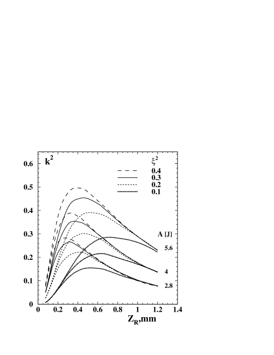
Figure 9: Square of the conversion probability (proportional to the $\gamma\gamma$ luminosity) as a function of the Rayleigh length for various parameters $\xi^{2}$ and laser flash energies; $x=4.8,\lambda=1.06\,\mu\mathrm{m}$ are assumed. The mirror system is situated outside the electron beam trajectories (collision angle $\theta=2\sigma_{L,x^{\prime}}$). The crab crossing angle $30\,{mrad}$ is taken into account. See also the text.

It was assumed that the angle between the laser optical axis and the electron beam line is $\theta=2\sigma_{L,x^{\prime}}$, where $\sigma_{L,x^{\prime}}$ is the angular divergence of the laser beam in the conversion region (eq. 17), and the mirror system is situated outside the electron beam trajectories. One conversion length corresponds to $k^{2}=(1-e^{-1})^{2}\approx 0.4$. One can see that $k^{2}=0.4$ at $\xi^{2}=0.3$ can be achieved with the minimum flash energy $A=5\,\mathrm{J}$. The optimum value of $Z_{R}$ is about 0.35$\,\mathrm{mm}$.

The r.m.s. duration of the laser pulse can be found from (21), for the considered case $\sigma_{L,z}=0.44\,\mathrm{mm}$ or 1.5$\,\mathrm{ps}$.

Above we have considered the requirements for the laser at $\lambda=1.06$ $x\approx 4.8$, which is the case for a $2E_{0}=500\,\mathrm{GeV}$ collider. The required flash energy as about 5$\,\mathrm{J}$ for $\xi^{2}=0.3$. Next we discuss what changes when the electron beam energy is decreased or increased?

When we decrease the energy to $E_{0}=100\,\mathrm{GeV}$, keeping the laser wavelength constant, the Compton cross section increases from $\sigma_{C}/\sigma_{0}=0.7$ ($x=4.8$) to 1.24 ($x=1.8$). This case corresponds to $W_{\gamma\gamma,m}\approx 130\,\mathrm{GeV}$. Calculations similar to the one presented in Fig. 9 show that for this case $k^{2}=0.4$ can be obtained with $A\approx 3.8\,\mathrm{J}$ at $\xi^{2}=0.1$ (and $Z_{r}\approx 0.6\,\mathrm{mm}$) or with $A\approx 2.5\,\mathrm{J}$ at $\xi^{2}=0.3$ (and $Z_{r}\approx 0.3\,\mathrm{mm}$). So, for the study of the low mass Higgs one needs a laser with somewhat lower flash energy and values of $\xi^{2}$ can be lower than that at $x\approx 4.8$.

Another variant for study of $W_{\gamma\gamma,m}\approx 130\,\mathrm{GeV}$ involves decreasing the electron beam energy keeping $x=const=4.8$. This requires $\lambda=1.06/3\,\mu\mathrm{m}$. Calculations show that using a 5$\,\mathrm{J}$ laser flash one can obtain only $k^{2}=0.35$ at $\xi^{2}=0.3$. The conversion coefficient is lower than that for $x=4.8$ and $\lambda=1.06$. This result is quite surprising, because for the shorter wavelength the nonlinear effects are less important and according to (20) the minimum flash energy does not depend on the wavelength. Such behaviour is connected with the effective transverse electron bunch size due to the crab–crossing (see above) which restricts the minimum laser spot size, and to the fact that for shorter wavelength the energy of each photon is larger.

Comparing the two methods of reaching the low mass Higgs region we come to the conclusion that it is easier to use a $\lambda=const=1.06\,\mu\mathrm{m}$ laser due to the lower flash energy, lower $\xi^{2}$ and the fact that this is the region of powerful solid state lasers (production of the second or third harmonics require $2$–$3$ times larger initial flash energy). There are also some advantages for physics, namely, a high degree of linear polarisation.

In Section 1 it was shown that it is possible to work with a $\lambda=1.06\,\mu\mathrm{m}$ laser even at the maximum TESLA energy of $2E_{0}=800\,\mathrm{GeV}$, in spite of a value of $x=7.17$. This is due to the nonlinear effects which increase the threshold for $e^{+}e^{-}$ pair production from $x=4.8$ to $x=4.8(1+\xi^{2})$. The Compton cross section for the value of $x=7.17$ is lower than at $x=4.8$ by a factor of 1.32. Nevertheless, with 5$\,\mathrm{J}$ flash energy and $\xi^{2}=0.4$, one can obtain $k^{2}\approx 0.35$.

So, we can conclude that a laser with $\lambda\approx 1\,\mu\mathrm{m}$ is suitable for all TESLA energies.

Summary of requirements to the laser

From the above considerations it follows that to obtain a conversion probability of $k\approx 63\%$ at all TESLA energies a laser with the following parameters is required:

Flash energy	$\approx 5\,\mathrm{J}$
Duration	$\tau(rms)\approx 1.5\,\mathrm{ps}$
Repetition rate	TESLA collision rate, $\approx 14\,\mathrm{kHz}$
Average power	$\approx 140\,\mathrm{kW}$ (for one pass collision)
Wavelength	$\approx 1\,\mu\mathrm{m}$ (for all energies).

4 The Interaction Region

1 The collision scheme, crab–crossing

The basic scheme for photon colliders is shown in Fig. 1 (Section 1). The distance between the conversion point (CP) and the IP, $b$, is chosen from the relation $b\approx\gamma\sigma_{y}$, so that the size of the photon beam at the IP has equal contributions from the electron beam size and the angular spread from Compton scattering. At TESLA $\sigma_{y}\approx 4\,\mathrm{nm}$ gives $b\approx 2\,\mathrm{mm}$ at $2E_{0}=500\,\mathrm{GeV}$. Larger $b$ values lead to a decrease of the $\gamma\gamma$ luminosity, for smaller $b$ values the low–energy photons give a larger contribution to the luminosity (which is not useful for the experiment but causes additional backgrounds).

In the TESLA Conceptual Design four years ago two schemes were considered: with magnetic deflection and without. At that time $\sigma_{y}$ was assumed to be about $16\,\mathrm{nm}$, and the distance $b\approx 1\,\mathrm{cm}$ was sufficient for deflection of the electron beam from the IP using a small magnet with $B\approx 5\,\mathrm{kG}$. With the new TESLA parameters with $b$ about 5 times smaller this option is practically impossible (may be only for a special experiment with reduced luminosity). We now consider only one scheme: without magnetic deflection, when all particles after the conversion region travel to the IP producing a mixture of $\gamma\gamma$, $\gamma e$, $e^{-}$$e^{-}$ collisions. The beam repulsion leads to some reduction of the $\gamma e$ luminosity and a considerable suppression of the $e^{-}e^{-}$ luminosity.

There are two additional constraints on the CP–IP distance. It should be larger than the half-length of the conversion region (which is about $Z_{R}\approx 0.35\,\mathrm{mm}$ (Section 3)), and larger than about $2$–$3$ $\sigma_{z}$ ($\sigma_{z}$ is the electron bunch length) because the $e\to\gamma$ conversion should take place before the beginning of electron beam repulsion. So, the minimum distance $b$ for the TESLA is about $1\,\mathrm{mm}$.

The removal of the disrupted beams can best be done using the crab-crossing scheme [182], Fig. 1, which is foreseen in the NLC and JLC projects for $e^{+}e^{-}$ collisions. In this scheme the electron bunches are tilted (using an RF cavity) with respect to the direction of the beam motion, and the luminosity is then the same as for head–on collisions. Due to the collision angle the outgoing disrupted beams travel outside the final quads. The value of the crab–crossing angle is determined by the disruption angles (see the next section) and by the final quad design (diameter of the quad and its distance from the IP). In the present TESLA design $\alpha_{c}=34\,\mathrm{mrad}$.

2 Collision effects in $\bgamma\bgamma$, $\bgamma$e collisions

The luminosity in $\gamma\gamma$,$\gamma e$ collisions may be limited by several factors:

• geometric luminosity of the electron beams;

• collision effects (coherent pair creation, beamstrahlung, beam displacement);

• beam collision induced background (large disruption angles of soft particles);

• luminosity induced background (hadron production, $e^{+}e^{-}$ pair production).

For optimisation of a photon collider it is useful to know qualitatively the main dependences. In this section we will consider collision effects which restrict the $\gamma\gamma$, $\gamma e$ luminosity.

Naively, at first sight, one may think that there are no collision effects in $\gamma\gamma$ and $\gamma e$ collisions because at least one of the beams is neutral. This is not correct because during the beam collision electrons and photons are influenced by the field of the opposite electron beam, which leads to the following effects [4, 5]:

$\gamma\gamma$ collisions: conversion of photons into $e^{+}e^{-}$ pairs (coherent pair creation).

$\gamma e$ collisions: coherent pair creation; beamstrahlung; beam displacement.

Below we consider the general features of these phenomena and then present the results of simulations where all main effects are included.

Coherent pair creation

The probability of pair creation per unit length by a photon with the energy $\omega$ in the magnetic field $B$ ($|B|+|E|$ for our case) is [4, 183]

$$\mu(\kappa)=\frac{\alpha^{2}}{r_{e}}\frac{B}{B_{0}}T(\kappa),\;\;\;\kappa=\frac{\omega}{mc^{2}}\frac{B}{B_{0}},\;\;B_{0}=\frac{\alpha e}{r_{e}^{2}}=4.4\cdot 10^{13}\;\mbox{G},$$ (1)

where $B_{0}$ is the the critical field, the function $T(\kappa)\approx 0.16\kappa^{-1}K^{2}_{1/3}(4/3\kappa)$. At $\kappa<1$, it is small, $T\approx 0.23\exp(-8/3\kappa)$, and $T\approx 0.1$ at $\kappa=3$–$10$.

In our case, $\omega\approx 0.8E_{0}$ , therefore one can put $\kappa\approx 0.8\Upsilon\equiv\gamma B/B_{0}$.

Coherent pair creation is exponentially suppressed for $\Upsilon<1$, but for $\Upsilon>1$ most high energy photons can convert to $e^{+}e^{-}$ pairs during the beam collision. The detailed analyses of these phenomena at photon colliders are presented in [4, 5, 184].

Without disruption the beam field $B\approx eN/(\sigma_{x}\sigma_{z})$ (we assume that $\sigma_{x}>\sigma_{y}$). Therefore, coherent $e^{+}e^{-}$ creation restricts the minimum horizontal beam size.

For example, for $N=2\times 10^{10}$, $\sigma_{x}=50\,\mathrm{nm}$, $\sigma_{z}=0.3\,\mathrm{mm}$, $E_{0}=500\,\mathrm{GeV}$, we obtain $\kappa_{av}\approx 1.2$, $T\approx 0.01$ and the $\gamma\to e^{+}e^{-}$ conversion probability $p\approx\mu\sigma_{z}=0.06$ (rather small). For $\sigma_{x}=10\,\mathrm{nm}$ it would be about 0.5 (40% loss of the $\gamma\gamma$ luminosity).

However, it turns out that at TESLA energies and beam parameters $N,\sigma_{z}$ the coherent pair creation is further suppressed due to the repulsion of the electron beams [185, 184]. Due to the repulsion, the characteristic size of the disrupted beam $r\approx\sqrt{\sigma_{z}r_{e}N/8\gamma}$, would be about $45\,\mathrm{nm}$ for the previous example. Therefore, with decreasing $\sigma_{x}$ the field at the IP increases to a maximum value $B\approx 2eN/(r\sigma_{z})$. The corresponding parameter $\Upsilon\propto(E_{0}/\sigma_{z})^{3/2}N^{1/2}$. As a result, at a sufficiently low beam energy and long beams the field may be below the threshold for coherent pair creation even for zero initial transverse beam sizes. This fact allows, in principle, very high $\gamma\gamma$ luminosity to be reached. This interesting effect is confirmed by the simulation [184] (Section 4).

One comment on the previous paragraph: although the beam disruption helps to suppress the coherent pair creation and to keep the $\gamma\gamma$ luminosity close to the geometric one, there is, nevertheless, some restriction on the field strength due to background caused by coherent pair creation. One can show that the minimum energy of electrons (at the level of probability of $W\approx 10^{-7}$) in coherent pair creation is about $E_{min}/\omega\approx 0.05/\kappa$. Therefore at $\kappa>2$ this energy is lower than the minimum energy of electrons after multiple Compton scattering and the resulting disruption angles will be determined by the coherent pair creation.

Electrons of similarly low energies are also produced in hard beamstrahlung with approximately similar probability. However, in the TESLA case, beamstrahlung is less important because electrons radiate inside the disrupted beam, while in the case of coherent pair creation the head of the Compton photon bunch travels in the field of the undisturbed oncoming electron beam and passes the region with the maximum (undisturbed) beam field. Simulation results for luminosity and disruption angles taking of all these effects into account are presented in Section 4.

Beamstrahlung

The physics of beamstrahlung (radiation during beam collisions) at linear $e^{+}e^{-}$ colliders is very well understood [186, 187]. Consequences of beamstrahlung for $\gamma\gamma$, $\gamma e$ colliders have been considered in [4, 5].

For $\gamma\gamma$ collisions beamstrahlung is not important. However, beamstrahlung photons collide with opposing Compton and beamstrahlung photons, increasing the total $\gamma\gamma$ luminosity by a significant factor (mainly in the the region of rather low invariant masses, below the high energy luminosity peak.)

In the $\gamma e$ collisions beamstrahlung leads to a decrease of the electron energy and, as a result, the $\gamma e$ luminosity in the high energy peak also decreases. In addition, the beamstrahlung photon contribution to the $\gamma e$ luminosity considerably worsens the $\gamma e$ luminosity spectrum.

Beam–beam repulsion

During the collision opposing beams either attract or repulse each other. In $e^{+}e^{-}$ collisions this effect leads to some increase of the luminosity (the pinch effect), while in $e^{-}e^{-}$ collisions the attainable luminosity is reduced [188, 189, 190].

Photon colliders are based on $e^{-}e^{-}$ beams. For $\gamma\gamma$ collisions the effects of the beam repulsion are only positive: the coherent pair creation is suppressed; the beamstrahlung photons emitted by the deflected electrons have a smaller probability of colliding with the Compton or beamstrahlung photons from the opposite electron beam; $\gamma e$ background is smaller due to the relative shift of the electron beams.

For $\gamma e$ collisions the effect of beam repulsion is negative. It leads to a displacement of the electron beam, and hence to a decrease of the $\gamma e$ luminosity.

The beam repulsion also leads to a considerable decrease of the $e^{-}e^{-}$ “background” luminosity.

Beam–beam deflection is very useful for the diagnostics of beam collisions and for the stabilisation of the luminosity both at $e^{+}e^{-}$ and photon photon colliders.

Depolarisation

Depolarisation effects are not included in our simulation code, therefore we give an estimation of these effects [4].

Depolarisation of electrons

When an electron is bent by the angle $\theta$, its spin rotates, relative to its trajectory, by the angle [170]

$$\theta^{\prime}=\frac{\mu^{\prime}}{\mu_{0}}\gamma\theta\approx\frac{\alpha\gamma}{2\pi}\theta,$$ (2)

where $\mu_{0}$ and $\mu^{\prime}$ are the normal and the anomalous magnetic moments of the electron, $\alpha=e^{2}/\hbar c=1/137$.

In the absence of disruption, the beam field

$$B\approx\frac{eN}{\sigma_{z}\sigma_{x}}.$$ (3)

The bending angle during beam collisions (on the length $\sigma_{z}$) is $\theta\approx eB\sigma_{z}/E_{0}=r_{e}N/(\sigma_{x}\gamma)$. This gives

$$\theta^{\prime}\approx\frac{\alpha r_{e}N}{2\pi\sigma_{x}}.$$ (4)

For example, for TESLA with $N=2\times 10^{10},\;\sigma_{x}\approx 100\,\mathrm{nm}$, we get $\theta^{\prime}=0.65$. The corresponding polarisation (for $\lambda_{e,0}=1$) is $\lambda_{e}\approx\cos{\;\theta^{\prime}}\approx 0.8$. The effect is not small.

Let us now consider the same case with beam repulsion taken into account. In $\gamma e$ collisions, the electrons collide with the high energy photons until their vertical displacement is smaller then $\sigma_{y}$ (this is the case with the high energy photons for $b=\gamma\sigma_{z}$ (see Section 1)). The deflection angles are derived from $\rho\theta^{2}/2\approx\sigma_{y}$ and $\rho\approx\gamma mc^{2}/eB$. This gives

$$\theta^{\prime}\approx\frac{\alpha\gamma}{2\pi}\sqrt{\frac{2\sigma_{y}r_{e}N}{\sigma_{x}\sigma_{z}\gamma}}.$$ (5)

For the previous set of parameters and $\sigma_{y}=4\,\mathrm{nm}$, $2E_{0}=500\,\mathrm{GeV}$, we obtain $\theta^{\prime}=0.1$ and $\lambda_{e}\approx\cos{\;\theta^{\prime}}\approx 0.995$.

Although this estimate is rough, one can see that a factor of $2$–$3$ will not change the conclusion that the Depolarisation of electrons in $\gamma e$ collisions is negligible.

Depolarisation of photons

It is well known that a strong electromagnetic field can be treated as an anisotropic medium with some refraction index $n$ [170]. In fact, the conversion of photons to $e^{+}e^{-}$ pairs (absorption) considered above is the manifestation of the imaginary part of the refraction index. The values $n$ are different for photons with linear polarisation parallel and perpendicular to the field direction. As a result, the polarisation of photons travelling in this field can change. In Section 1 we mentioned already one such effect in the conversion region. Here we will consider the influence of the beam field on the polarisation of the high energy photons.

Figure 1: Decrease in photon helicity during beam collisions for various beam parameters and probabilities of coherent pair creation $W_{e^{+}e^{-}}$ [177, 178]. See comments in the text.

This problem was considered in detail in [177, 178]. The beam field can transform the circular photon polarisation into a linear polarisation and vice versa. The degree of Depolarisation as a function of $E_{\gamma}/\sigma_{z}$ is shown in Fig. 1. Instead of the field strength each curve corresponds to a certain value of the coherent pair creation probability $W_{e^{+}e^{-}}$ which is defined in units of collision lengths. In this case, consideration of the beam disruption is not necessary, as it is included in the $e^{+}e^{-}$ conversion probability which is kept under control at photon colliders.

For example, for TESLA beams $E_{\gamma}/\sigma_{z}\approx 10\,\mathrm{TeV}/\mathrm{cm}$. We see that even for 50% $e^{+}e^{-}$ conversion probability the decrease of the photon polarisation is only about 1%. Moreover, as was mentioned before, due to the beam repulsion the coherent pair creation probability at TESLA is small, therefore the Depolarisation will be even smaller. Hence, the Depolarisation of photons is negligibly small.

Disruption angle

The maximum disruption angle is an important issue for photon colliders, it determines the value of the crab–crossing angle.

One source of large angle particles are low energy electrons from the conversion region. The minimum energy is about $0.02E_{0}$ (section 1). The second source of soft particles is hard beamstrahlung and coherent pair creation with the minimum energy of about $0.05/\Upsilon$. Particles from these sources can carry very large energies, therefore the crab–crossing angle should be sufficient for removal of all these particles from the detector without hitting the quads or detector components.

Another source of even lower energy particles are $e^{+}e^{-}$ pairs produced incoherently in collisions of individual particles at the IP. This unavoidable background is proportional to the luminosity. A large fraction of these particles (with large energy and small angles) can also escape from the detector through the exit hole for disrupted beams. This source of background carries much less power than enumerated in the previous paragraph and can be handled without crab–crossing, as in the $e^{+}e^{-}$ TESLA option.

The deflection angle for soft electrons in the field of the opposite beam is given approximately by [4, 19]

$$\vartheta_{d}\approx 0.7\left(\frac{4\pi r_{e}N}{\sigma_{z}\gamma_{min}}\right)^{1/2}\approx 9\left(\frac{N/10^{10}}{\sigma_{z}[\mathrm{mm}]E_{min}[\mathrm{GeV}]}\right)^{1/2}\,\mathrm{mrad}.$$ (6)

In the first approximation the deflection angle for very soft electrons does not depend on the transverse beam size. The coefficient 0.7 here was found by tracking particles in the field of the beam with a Gaussian longitudinal distribution for the TESLA range of parameters. For example: at $2E_{0}=500\,\mathrm{GeV}$, $E_{min}/E_{0}=0.02$ (Compton, $x=4.8$), $N=2\times 10^{10},\sigma_{z}=0.3\,\mathrm{mm}$ we get $\vartheta_{d}\approx 10.4\,\mathrm{mrad}$. This estimate will help us to understand results of the simulation.

The coefficient 0.7 in (6) corresponds to the collision of a low energy electron with the electron beam. If a low energy electron is produced near the centre of the opposing beam then it is more accurate to use the coefficient 1.2 instead of 0.7.

3 The simulation code

As we have seen, the picture of beam collisions at photon colliders is complicated and the best way to obtain final results is a simulation. In the present study we used the code described in [5].

It serves for simulation of $e^{+}e^{-}$, $e^{-}e^{-}$, $\gamma e$, $\gamma\gamma$ beam collisions in linear colliders and the present version takes into account the following processes:

1. Compton scattering in the conversion region. At present we use the formulae for linear Compton scattering, including all polarisation effects. Nonlinear effects are considered approximately by smearing $x$ ($x\to x/(1+\xi^{2})$) according to the variable density of laser photons in the conversion region.

2. $e^{+}e^{-}$ pair creation in the conversion region for $x>4.8$.

3. Deflection by magnetic fields and synchrotron radiation in the region between the CP and IP, due to special magnets or the solenoidal detector field (it has an effect due to the crab–crossing angle).

4. Electromagnetic forces, coherent pair creation and beamstrahlung during beam collisions at the IP.

5. Incoherent $e^{+}e^{-}$ creation in $\gamma\gamma$, $\gamma e$, $e^{+}e^{-}$ collisions.

The initial electron beams are described by about 3000 macro–particles (m.p.) which have a shape of flat rectangular bars with the horizontal size equal to 0.4$\sigma_{x}$ and zero vertical size. In the longitudinal direction the electron bunch has a Gaussian shape ($\pm 3\sigma$) and is cut into about 150 slices. It is assumed that the macro–particles have only a transverse field and influence macro–particles of the opposite bunch which have the same z–coordinate (this coordinate changes by steps). At initial positions macro–particles move to the collision region according to the beam emittances and beta functions. During the simulation new macro–particles (photons, electrons and positrons) are produced which are included in the calculation in the same way as the initial macro-particles.

Low energy particles can get too large a deflection during one step (because the step is too large). This problem is solved by artificial restriction of the deflection angle (and the corresponding transverse displacement) for one step. The resulting angles will be simulated correctly because the repulsion length for the soft electron is much shorter than the bunch length and the charge distribution (the beam field) in the next steps is approximately the same.

The code was used for simulation of photon colliders in NLC Zero Design and the TESLA Conceptual Design. The results are in agreement [191] with the code CAIN [192] written later for the same purpose.

4 Luminosity limitations due to beam collision effects

Beam collision effects in $e^{+}e^{-}$ and $\gamma\gamma$, $\gamma e$ collisions are different. In particular, in $\gamma\gamma$ collisions there are no beamstrahlung or beam instabilities. Therefore, it was of interest to study limitations of the luminosity at the TESLA photon collider due to beam collision effects. The simulation [9, 21] was done for the TESLA beams and the horizontal size of the electron beams was varied.

Ultimate luminosities

Fig. 2 shows the dependence of the $\gamma\gamma$ (solid curves) and the $\gamma e$ (dashed curves) luminosities on the horizontal beam size for several energies.

Figure 2: Dependence of $\gamma\gamma$ and $\gamma e$ luminosities in the high energy peak on the horizontal beam size for TESLA at various energies. See also comments in the text.

The horizontal beam size was varied by changing the horizontal beam emittance keeping the horizontal beta function at the IP constant and equal to $1.5\,\mathrm{mm}$.

One can see that all curves for the $\gamma\gamma$ luminosity follow their natural behaviour: $L\propto 1/\sigma_{x}$ (values of $\sigma_{x}<10\,\mathrm{nm}$ are not considered because too small horizontal sizes may introduce problems with the crab–crossing scheme). Note that while in $e^{+}e^{-}$ collisions $\sigma_{x}\approx 500\,\mathrm{nm}$, in $\gamma\gamma$ collisions the attainable $\sigma_{x}$ with the planned injector (damping ring) is about $100\,\mathrm{nm}$ (Section 5).

In $\gamma e$ collisions the luminosity at small $\sigma_{x}$ is lower than follows from the geometric scaling due to beamstrahlung and displacement of the electron beam during the beam collision. So, we can conclude that for $\gamma\gamma$ collisions at TESLA one can use beams with a horizontal beam size down to $10\,\mathrm{nm}$ (maybe even smaller) which is much smaller than that in $e^{+}e^{-}$ collisions. Note, that the vertical beam size could also be additionally decreased by a factor of two (for even smaller electron beam size the effective photon beam size will be determined by the Compton scattering contribution). As a result, the $\gamma\gamma$ luminosity in the high energy peak can be, in principle, several times higher than the $e^{+}e^{-}$ luminosity (Table 1).

Production of the polarised electron beams with emittances lower than those possible with damping rings is a challenging problem. There is one method, laser cooling [193, 194, 195] which allows, in principle, the required emittances to be reached. However this method requires a laser power one order of magnitude higher than is needed for $e\to\gamma$ conversion. This is not excluded, but since many years of R&D would be required, it should be considered as a second stage of the photon collider, maybe for a Higgs factory.

Disruption angles

As it was mentioned before, for small beam sizes one can expect the production of low energy particles in the processes of coherent pair creation and beamstrahlung. The luminosity may not be affected, but there is the problem with background due to the deflection of the low energy particles by the opposing electron beam.

Figure 3: Dependence of the maximum disruption angle on the horizontal beam size for TESLA at various energies. Left figure for $x=4.8$ and several beam energies. Right figure corresponds to the invariant mass $W_{\gamma\gamma}=105\,{GeV}$, $x$ values $1.6$, $2.7$, $3.75$ correspond to the laser wave lengths $1.06$, $1.06/2$, $1.06/3\,\mu\mathrm{m}$, respectively.

Fig. 3 shows the dependence of the maximum disruption angle on the horizontal beam size. In the left figure the parameter $x=4.8$, the right figure corresponds to the c.m.s. energy of the $\gamma\gamma$ collider equal to $105\,\mathrm{GeV}$. The total statistics in the simulation is about $10^{5}$ particles, so the tails which can lead to background are not simulated. However, we know the scaling and therefore can make corrections. From the simulation we have found the angle corresponding to the probability $10^{-4}$ and multiplied it by a factor of 1.25. The angle shown in Fig. 3 is the angle above which the energy of background particles is less than about $10\,\mathrm{TeV}$, that is less than the energy of the incoherent $e^{+}e^{-}$ pairs (Section 7) which have larger angles and represent an unavoidable background.

In Fig. 3 (left) we see that at large $\sigma_{x}$ the angle is smaller for higher beam energies, in agreement with (6). With decreasing $\sigma_{x}$ the contribution of the low energy particles from coherent pair creation and beamstrahlung is seen.

Fig. 3 (right) shows that at the fixed $\gamma\gamma$ center–of–mass energy $W_{\gamma\gamma}$ the disruption angle is larger for larger $x$. It is easy to show that

$$\vartheta\propto\frac{x}{\sqrt{(x+1)\sigma_{c}(x)}},$$ (7)

where the Compton cross section $\sigma_{c}(x)$ decreases with increasing $x$. This gives a factor of two difference between $x=1.6$ and $3.75$. We think that one can study the low mass Higgs with $\lambda\approx 1.06\,\mu\mathrm{m}$, i.e. with the same laser at all energies below $2E_{0}=500\,\mathrm{GeV}$. Lower $x$ have the advantage of a higher degree of linear polarisation (Section 1). As higher $x$ values also have also some advantages (sharper edge) we can foresee the possibility of a frequency doubled laser. With these assumptions we conclude that the maximum disruption angle is about $14\,\mathrm{mrad}$. For the laser with $\lambda\approx 1\,\mu\mathrm{m}$ $12\,\mathrm{mrad}$ will be sufficient. In the present design the crab–crossing angle in the second IP is $34\,\mathrm{mrad}$. These values put restrictions on possible quadrupole designs.

5 $\bgamma\bgamma$ and $\bgamma$e luminosities at TESLA

Parameters of the electron beams

In this section we discuss what luminosities can be obtained with the technology presently available. It depends strongly on the emittances of the electron beams. There are two methods of production, low–emittance electron beams: damping rings and low–emittance RF–photo–guns (without damping rings). The second option is promising, but at the moment there are no such photo–guns producing polarised electron beams [196]. Polarisation of electron beams is very desirable for photon colliders (sect 2). So, there is only one choice now — damping rings.

Especially for a photon collider the possibility of decreasing the beam emittances at the TESLA damping ring has been studied [197] and it was found that the horizontal emittance can be reduced by a factor of 4 compared to the previous design. Now the normalised horizontal emittance is $\mbox{$\epsilon_{nx}$}\ =2.5\times 10^{-6}\,\mathrm{m}$.

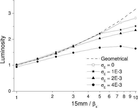
Figure 4: Dependence of the geometric $e^{-}e^{-}$ luminosity on the horizontal $\beta$–function (SLAC design). For TESLA the relative energy spread ($\sigma_{E}$ in the figure) is $10^{-3}$.

The luminosity also depends on the $\beta$–functions at the interaction points: $L\propto 1/\sqrt{\beta_{x}\beta_{y}}$. The vertical $\beta_{y}$ is usually chosen close to the bunch length $\sigma_{z}$ (this is the design for $e^{+}e^{-}$ collisions and can also be realized for $\gamma\gamma$ collisions). Some questions remain about the minimum horizontal $\beta$–function. For $e^{+}e^{-}$ collisions, $\beta_{x}\approx 15\,\mathrm{mm}$ which is larger than the bunch length $\sigma_{z}=0.3\,\mathrm{mm}$, because beams in $e^{+}e^{-}$ collisions must be flat to reduce beamstrahlung. In $\gamma\gamma$ collisions, $\beta_{x}$ could be about $1\,\mathrm{mm}$ (or even somewhat smaller). There are two fundamental limitations: the beam length and the Oide effects [198] (radiation in final quads). The latter is not important for the beam parameters considered. There is also a certain problem with the angular spread of the synchrotron radiation emitted in the final quads. But, for the photon collider the crab–crossing scheme will be used and in this case there is sufficient clearance for the removal of the disrupted beams and synchrotron radiation.

Very preliminary studies of the existing scheme for the TESLA final focus have shown [199] that chromo–geometric aberrations dominate at $\beta\leq 6\,\mathrm{mm}$. However, this is not a fundamental limitation and it is very likely that after further study and optimisation a better solution will be found. At SLAC a new scheme for the final focus system has recently been proposed [200]. The first check without optimisation has shown [201] that, with the new scheme, one can obtain $\beta_{x}\approx 1.5\,\mathrm{mm}$ with small aberrations, see Fig. 4, and further optimisation is possible. For the present study we assume $\beta_{x}=1.5\,\mathrm{mm}$.

Some uncertainties remain for the operation of TESLA at low energies. For the low mass Higgs the minimum required energy is about $75\,\mathrm{GeV}$. In this case TESLA should work either at reduced accelerating gradient or a bypass after about $100\,\mathrm{GeV}$ should be used. In the case of a bypass one can consider that the luminosity is approximately proportional to the beam energy (due to the adiabatic change of the beam emittances).

In principle, the loss of luminosity at low energies could be compensated by an increase of the repetition rate as $f\propto 1/E_{0}$. In this case the RF power (for the linac) is constant. However, for the present design of the TESLA damping ring, the repetition rate may be increased at most by a factor of 2. Further decrease of the damping time is possible but at additional cost (wigglers, RF–power). The factor of 2 is almost sufficient, but, unfortunately, at low gradients beam loading (RF efficiency) may be problem. Its adjustment requires the change of the coupler position, which for TESLA is technically very difficult or even impossible.

For the present study we assume the bypass solution and use the same beam parameters ($N,\sigma_{z}$, normalised emittances, collision rate) for all energies, that gives $L\propto E_{0}$.

$\bgamma\bgamma$, $\bgamma$e luminosities, summary table

The resulting parameters of the photon collider at TESLA for $2E_{0}=$ $200$, $500$ and $800\,\mathrm{GeV}$ are presented in Table 1. It is assumed that the electron beams have 85% longitudinal polarisation and that the laser photons have 100% circular polarisation. The thickness of the laser target is one scattering length for $2E_{0}=500$ and $800\,\mathrm{GeV}$ and 1.35 scattering length for $2E_{0}=200\,\mathrm{GeV}$ (the Compton cross section is larger), so that $k^{2}\approx$ 0.4 and 0.55, respectively. The parameter $\xi^{2}=0.15,0.3,0.4$ for $2E_{0}=200,$ $500$, $800\,\mathrm{GeV}$, as explained in Section 2. The laser wave length is $1.06\,\mu\mathrm{m}$ for all energies. The conversion point is situated at a distance $b=\gamma\sigma_{y}$ from the interaction point.

$2E_{0}$ [GeV]	200	500	800
$\lambda_{L}$ [$\,\mu\mathrm{m}$]/$x$	1.06/1.8	1.06/4.5	1.06/7.2
$t_{L}$ $[\lambda_{scat}]$	1.35	1	1
$N/10^{10}$	2	2	2
$\sigma_{z}$ [mm]	0.3	0.3	0.3
$f_{rep}\times n_{b}$ [kHz]	14.1	14.1	14.1
$\gamma\epsilon_{x/y}/10^{-6}$ [m$\cdot$rad]	2.5/0.03	2.5/0.03	2.5/0.03
$\beta_{x/y}$ [mm] at IP	1.5/0.3	1.5/0.3	1.5/0.3
$\sigma_{x/y}$ [nm]	140/6.8	88/4.3	69/3.4
b [mm]	2.6	2.1	2.7
$L_{ee}\,(geom)$ [$10^{34}$  $\,\mathrm{cm^{-2}s^{-1}}$]	4.8	12	19
$L_{\gamma\gamma}(z>0.8z_{m,\gamma\gamma\ })[10^{34}\,\mathrm{cm^{-2}s^{-1}}]$	0.43	1.1	1.7
$L_{\gamma e}(z>0.8z_{m,\gamma e\ })[10^{34}\,\mathrm{cm^{-2}s^{-1}}]$	0.36	0.94	1.3
$L_{e^{-}e^{-}}(z>0.65)[10^{34}\,\mathrm{cm^{-2}s^{-1}}]$	0.03	0.07	0.095

Table 1: Parameters of the $\gamma\gamma$ collider based on TESLA.

Figure 5: $\gamma\gamma$ luminosity spectra at TESLA(500) with various cuts on longitudinal momentum. Solid line for total helicity of the two photons 0 and dotted line for total helicity 2. See also Table 1.

As it was already mentioned in the introduction, for the same energy

$$L_{\gamma\gamma}(z>0.8z_{m})\approx\frac{1}{3}L_{e^{+}e^{-}}.$$ (8)

The relation (8) is valid only for the beam parameters considered. A more universal relation is (for $k^{2}=0.4$)

$$L_{\gamma\gamma}(z>0.8z_{m})\approx 0.09L_{ee}(geom).$$ (9)

The normalised $\gamma\gamma$ luminosity spectra for 2E${}_{0}=500\,\mathrm{GeV}$ are shown in Fig. 5 [21].

The luminosity spectrum is decomposed into two parts with the total helicity of the two photons 0 and 2. We see that in the high energy part of the luminosity spectra the photons have a high degree of polarisation. In addition to the high energy peak, there is a factor $5$–$8$ higher luminosity at low energy. It is produced mainly by photons after multiple Compton scattering and beamstrahlung photons. These events have a large boost and can be easily distinguished from the central high energy events. Fig. 5 shows the same spectrum with an additional cut on the longitudinal momentum of the produced system, which suppresses the low energy luminosity to a low level. For two jet events ($H\to b\bar{b},\;\tau\tau$, for example) one can restrict the longitudinal momentum using the acollinearity angle between the jets. The resulting energy spread of collisions can be about 7.5%, see Fig. 5 (right).

Figure 6: Left: normalised $\gamma e$ luminosity spectra at TESLA(500) when the photon collider is optimised for $\gamma\gamma$ collisions and there is $\gamma\to e$ conversion for both electron beams, parameters are given in table 1. Right figure: there is $\gamma\to e$ conversion only for one electron beam and the distance between interaction and conversion point is 1.7$\,\mathrm{cm}$. See comments in the text.

Figure 7: The $\gamma\gamma$ luminosity spectra at TESLA for $2E_{0}=800$ and $200\,\mathrm{GeV}$ (for Higgs(120)) with various cuts on longitudinal momentum (the case of $2E_{0}=500\,{GeV}$ is shown in Fig. 5). The solid line is for the total helicity of the two photons 0 and the dotted line for the total helicity 2. See also Table 1.

The high energy part of the $\gamma\gamma$ luminosity spectrum is almost independent of collision effects at the IP (beamstrahlung and multiple Compton scattering). For theoretical studies one can calculate the high energy part of the luminosity spectrum with sufficient accuracy by convolution of the Compton function [3]. Recently, a simple analytical formula for the Compton spectrum has been obtained [174] which takes into account nonlinear effects in the conversion region for sufficiently small values of $\xi^{2}$.

The normalised $\gamma e$ luminosity spectra for $2E_{0}=500\,\mathrm{GeV}$ are shown in Fig. 6(left). Again, besides the high energy peak there is a several times higher $\gamma e$ luminosity at low invariant masses. Note, that the $\gamma e$ luminosity in the high energy peak is not a simple geometric characteristic of the Compton scattering process (as it is in $\gamma\gamma$ collisions). For the case considered it is suppressed by a factor of $2$–$3$, mainly due to the repulsion of the electron beams and beamstrahlung. The suppression factor depends strongly on the electron beam parameters.

For dedicated $\gamma e$ experiments one can convert only one electron beam, increase the distance between the conversion and the interaction points and obtain a much more monochromatic $\gamma e$ luminosity spectrum. One of such examples is shown in Fig. 6(right).

The luminosity distributions for $2E_{0}=800\,\mathrm{GeV}$ is presented in Fig. 7 (left), and for $2E_{0}=200\,\mathrm{GeV}$ on Fig. 7 (right). The latter case corresponds to $W_{\gamma\gamma,m}\approx 120\,\mathrm{GeV}$. At $2E_{0}=800\,\mathrm{GeV}$ the value $x\approx 7.2>4.8$, however, due to nonlinear effects in the conversion region there is no suppression of the luminosity which might be due to $e^{+}e^{-}$ creation (Section 1).

For the Higgs the production rate is proportional to $dL_{0}/dW_{\gamma\gamma}$ at $W_{\gamma\gamma}=M_{H}$. For the case considered, $M_{H}\approx 120\,\mathrm{GeV}$, and $x=1.8$, $dL_{0}/dW_{\gamma\gamma}=1.87\times 10^{32}\,\mathrm{cm^{-2}s^{-1}}/\,\mathrm{GeV},$ so that the coefficient in Fig. 5 characterising the width of the peak is about 5.3 (instead of 7).

Several other important accelerator aspects of the photon collider at TESLA are discussed in [199].

6 Monitoring and measurement of the $\bgamma\bgamma$ and $\bgamma$e luminosities

Luminosity measurement in $\bgamma\bgamma$ collisions

At photon colliders the luminosity spectrum is broad, photons and electrons may have various polarisations. One should have method to measure all luminosity characteristics. Let us start from $\gamma\gamma$ collisions.

We consider the head-on collisions of photons with 4–momenta $k_{1,2}$ and energies $\omega_{1,2}$. The $z$–axis is chosen along the momentum of the first photon, all the azimuthal angles are referred to one fixed orthogonal $x$–axis. The polarisation properties of the i–th photon are described by three parameters: $\lambda_{i}$ the mean helicity (or degree of the circular polarisation), $l_{i}$ and $\gamma_{i}$ the mean degree of the linear polarisation and the azimuthal angle of its direction. The total cross section $\sigma$ for the $\gamma\gamma$ collisions after summing over polarisations of final particles has the form [175]

$$\sigma=\sigma^{np}+\lambda_{1}\lambda_{2}\;\tau^{c}+l_{1}l_{2}\;\tau^{l}\;\cos{2(\gamma_{1}-\gamma_{2})}$$ (10)

where $\sigma^{np}$ is the total cross section for unpolarised photons and $\tau^{c}$ ($\tau^{l}$) is the asymmetry related to the circularly (linearly) polarised photons. Besides, we use the notations $\sigma_{0}=\sigma^{np}+\tau^{c}$ and $\sigma_{2}=\sigma^{np}-\tau^{c}$ where $0$ and $2$ denote values of $|\lambda_{1}-\lambda_{2}|$ — the total helicity of the produced system. The system produced in a $\gamma\gamma$ collision is characterised by its invariant mass $W_{\gamma\gamma}=\sqrt{4\omega_{1}\omega_{2}}$ and rapidity $\eta=0.5\,\ln(\omega_{1}/\omega_{2})$.

Let us fist consider the important case when both photons are circularly polarised. In this case we should have a method to measure a spectral luminosity $dL/dW_{\gamma\gamma}d\eta$ and the product of helicities $\lambda_{1}\lambda_{2}$ or, in other words, the spectral luminosities $dL_{0}/dW_{\gamma\gamma}d\eta$ and $dL_{2}/dW_{\gamma\gamma}d\eta$ with the total helicity $0$ and $2$.

These luminosities can be measured using the process $\gamma\gamma\to l^{+}l^{-}$, where $l=e$ or $\mu$ [2, 202, 5, 203, 204]. The cross section of this process for colliding photons with total helicity $0$ and $2$ and for $W^{2}_{\gamma\gamma}\gg m^{2}$ is ($\hbar=c=1$)

$$\sigma_{0}(|\cos\vartheta|<a)\approx\frac{4\pi\alpha^{2}}{W^{2}_{\gamma\gamma}}{8m^{2}\over W^{2}_{\gamma\gamma}}\left[\frac{1}{2}\ln\left(\frac{1+a}{1-a}\right)+\frac{a}{1-a^{2}}\right]$$

$$\sigma_{2}(|\cos\vartheta|<a)\approx\frac{4\pi\alpha^{2}}{W^{2}_{\gamma\gamma}}\left[2\ln\left(\frac{1+a}{1-a}\right)-2a\right].$$ (11)

One can see that $\sigma_{0}/\sigma_{2}\sim m^{2}/W^{2}_{\gamma\gamma}\ll 1$ (excluding the region of small angles). For photons with arbitrary circular polarisations the cross section is

$$\sigma_{\gamma\gamma\to e^{+}e^{-}}=\frac{1+\lambda_{1}\lambda_{2}}{2}\sigma_{0}+\frac{1-\lambda_{1}\lambda_{2}}{2}\sigma_{2},$$ (12)

where $\sigma_{2}\gg\sigma_{0}$.

Hence the number of events

$$dN_{\gamma\gamma\to\mu^{+}\mu^{-}}\approx dL\,{1-\lambda_{1}\lambda_{2}\over 2}\,\sigma_{2}\equiv dL_{2}\,\sigma_{2}\,,$$ (13)

and one can measure the luminosity $dL_{2}/dW_{\gamma\gamma}d\eta$. Measurement of $dL_{0}/dW_{\gamma\gamma}d\eta$ is done by inversion of the helicity of one photon beam simultaneously changing the signs of the helicities of the laser beam used for the $e\to\gamma$ conversion and that of the electron beam [202]. In this case the spectrum of scattered photons is not changed while the product $\lambda_{1}\lambda_{2}$ changes its sign. In other words, $L_{0}$ ”becomes” now $L_{2}$, which is measurable. The cross section for this process is $\sigma(|\cos\vartheta|<0.9)\approx 10^{-36}/W^{2}_{\gamma\gamma}[\mathrm{TeV}]\,\mathrm{cm}^{2}$. This process is very easy to select due to a zero coplanarity angle.

Linear photon polarisations can also be measured using the above processes. At large angles the cross section has a strong correlation between the plane of the final state particles and the directions of the photon polarisations. Let us consider the general case in more detail.

The differential cross section can be written in the form [3]

$$d\sigma={\alpha^{2}\,T\over W^{2}_{\gamma\gamma}\,(m^{2}+{\bf p}_{-\bot}^{2})^{2}}\,d\Gamma\,,\;\;d\Gamma=\delta(k_{1}+k_{2}-p_{-}-p_{+}){d^{3}p_{-}d^{3}p_{+}\over E_{-}E_{+}}={dtd\varphi_{-}\over W^{2}_{\gamma\gamma}},$$ (14)

where ${\bf p}_{-\perp}$ is the transverse momentum of the electron, $t=(k_{1}-p_{-})^{2}$ and $\varphi_{-}$ is the azimuthal angle of the electron. The quantity $T$ is

$$T=T_{00}+\lambda_{1}\lambda_{2}\,T_{22}-2T_{\varphi}\,,$$ (15)

with

$$T_{00}=m^{2}(W^{2}_{\gamma\gamma}-2m^{2})+{\bf p}_{-\bot}^{2}(W^{2}_{\gamma\gamma}-2{\bf p}_{-\bot}^{2})\,,$$

$$T_{22}=m^{2}(W^{2}_{\gamma\gamma}-2m^{2})-{\bf p}_{-\bot}^{2}(W^{2}_{\gamma\gamma}-2{\bf p}_{-\bot}^{2})\,,$$ (16)

and

$$T_{\varphi}=l_{1}l_{2}\,[\,m^{4}\,\cos{(2\phi_{1}-2\phi_{2})}+({\bf p}_{-\bot}^{2})^{2}\cos{(2\phi_{1}+2\phi_{2})}\,]-$$

$$-2m^{2}{\bf p}_{-\bot}^{2}\,[\,l_{1}\,\cos{2\phi_{1}}+l_{2}\,\cos{2\phi_{2}}\,]\,,$$ (17)

where $\phi_{i}=\varphi_{-}-\gamma_{i}$ is the (azimuthal) angle between the vector ${\bf p}_{-\perp}$ and the direction of the linear polarisation of i-th photon (therefore, the angle $\phi_{2}-\phi_{1}=\gamma_{1}-\gamma_{2}$). From (15), ignoring the azimuthal term, the contribution of the total helicity 0 corresponds to the sum $T_{00}+T_{22}$ and the helicity 2 to the term $T_{00}-T_{22}$, which is smaller by a factor of $m^{2}/p^{2}_{\bot}$, in agreement with our previous observation (see 12).

At high energy and not too small angles the cross section is

$$d\sigma={\alpha^{2}\over W^{2}_{\gamma\gamma}}\,\left[(1-\lambda_{1}\lambda_{2})\left({W^{2}_{\gamma\gamma}\over{\bf p}_{-\bot}^{2}}-2\right)-2l_{1}\,l_{2}\,\cos(2\phi_{1}+2\phi_{2})\,\right]\,d\Gamma\,,$$ (18)

$$d\Gamma={2\omega_{1}\omega_{2}\over\left[\omega_{1}(1-\cos{\theta_{-}})+\omega_{2}(1+\cos{\theta_{-}})\right]^{2}}\,d\Omega_{-}\,,\;\;W^{2}_{\gamma\gamma}\gg m^{2},\quad{\bf p}_{-\bot}^{2}\gg m^{2}$$

where $d\Omega_{-}$ is the electron solid angle. One sees that at large angles ($p_{\bot}\sim W_{\gamma\gamma}/2$) the cross section depends strongly on the degrees of both the circular and the linear photon polarisations.

The cross section of the calibration processes $\gamma\gamma\ \to e^{+}e^{-}(\mu^{+}\mu^{-})$ is larger than those for most processes to be studied and only the processes $\gamma\gamma\to$W⁺W^- and $\gamma\gamma\ \to\mathrm{hadrons}$ have larger cross sections. However, taking the detection efficiency for WW into account, the counting rate of WW pairs will be comparable with that of the calibration processes. As for hadrons, the expected number of calibration events is sufficient to measure the properties of hadronic reactions with high accuracy.

Note that the momenta of electrons (muons) in the processes under discussion can be measured with a high accuracy which is very important for the determination of the luminosity distribution near the high energy edge.

Other processes with large cross sections which can be used for the luminosity measurement are $\gamma\gamma\ \to W^{+}W^{-}$ [204] and $\gamma\gamma\ \to\mu^{+}\mu^{-}\mu^{+}\mu^{-}$ [2, 205]. The first process has a total cross section of $8\times 10^{-35}\,\,\mathrm{cm}^{2}$ the second one $1.6\times 10^{-34}\,\,\mathrm{cm}^{2}$. The first process depends on the photon polarisations especially in the region of large angles [112, 113]. The second processes is sensitive only to the linear photon polarisation. These processes may be useful, for an independent check and a fast monitoring of the luminosity.

Luminosity measurement in $\bgamma$e collisions

For the absolute $\gamma e$ luminosity measurement, one can use the process of Compton scattering, which is strongly polarisation dependent.

Let us consider the polarisation properties of Compton scattering at high energies. For an $\gamma e$ collider we consider the head–on collision of an electron with 4–momentum $p$ and a photon with 4–momentum $k$, energies $E$ and $\omega$ of the same order and the squared invariant mass of $\gamma e$ system $W^{2}_{\gamma e}=(p+k)^{2}\approx 4E\omega$. We choose the $z$–axis along the momentum of the electron. The polarisation properties of the electron are described by its mean helicity $\lambda_{e}$ ($|\lambda_{e}|\leq 1/2$), transverse polarisation $\zeta_{\perp}$ ($\zeta_{\perp}\leq 1$), and the azimuthal angle $\beta$ of the direction of the transverse polarisation. The polarisation properties of the photon are described by three parameters: $\lambda_{\gamma}$ the mean helicity (or degree of the circular polarisation), $l_{\gamma}$ and $\gamma$ the mean degree and the direction of the linear polarisation.

The total and differential cross sections for the process $e(p)+\gamma(k)\to e(p^{\prime})+\gamma(k^{\prime})$ and their dependence on the polarisation of the initial particles are discussed in [3]. We consider here the case of high energies $W^{2}_{\gamma e}\gg m^{2}$ only. In this case the total cross section

$$\sigma\approx(1+2\lambda_{e}\lambda_{\gamma})\,{2\pi\alpha^{2}\over W^{2}_{\gamma e}}\,\ln{W^{2}_{\gamma e}\over m^{2}},\quad W^{2}_{\gamma e}\gg m^{2}$$ (19)

depends strongly on the circular photon polarisation and on the longitudinal electron polarisation only. Here the mean electron helicity is defined as a projection of its spin and 100% polarisation corresponds to $\lambda_{e}=1/2$.

The differential cross section depends on the degrees of the circular and linear polarisations of the photon and on its angle $\gamma$ which determines the direction of the linear photon polarisations as well as on the electron polarisation. It can be written in the the form

$$d\sigma={\alpha^{2}\,F_{0}\over m^{2}x\,}\,d\Gamma\,,\;\;d\Gamma=\delta(p+k-p^{\prime}-p^{\prime}){d^{3}p^{\prime}d^{3}k^{\prime}\over E^{\prime}\omega^{\prime}}={dyd\varphi_{\gamma}}$$ (20)

where

$$x={2pk\over m^{2}}\approx{4E\omega\over m^{2}}\gg 1\,,\;\;y=1-{pk^{\prime}\over pk}\,,\;\;r={y\over(1-y)x}$$

and $\varphi_{\gamma}$ is the azimuthal angle of the final photon. The quantity $F_{0}$ is

$$F_{0}={1\over 1-y}+1-y-4r(1-r)\left[1+l_{\gamma}\,\cos{2(\varphi-\gamma)}\right]-$$ (21)

$$-y\lambda_{\gamma}\left[2\sqrt{r(1-r)}\,\zeta_{\perp}\,\cos{(\varphi-\beta)}-{2-y\over 1-y}\,(1-2r)\,2\lambda_{e}\right]\,.$$

In the region of angles $\theta_{\gamma}\gg m/E$, we have

$$1-y={E(1-\cos{\theta_{\gamma}})\over E(1-\cos{\theta_{\gamma}})+\omega(1+\cos{\theta_{\gamma}})}\,,\;\;d\Gamma={2E\omega\over[E(1-\cos{\theta_{\gamma}})+\omega(1+\cos{\theta_{\gamma}})]^{2}}\,d\Omega_{\gamma}\,.$$ (22)

If the angle $\theta_{\gamma}\approx 1$ all terms in expression (21) have to be taken into account. Thus by detecting the final state particles at large angles, one can measure all polarisation parameters of the colliding particles.

In the region ${m/E}\ll\theta_{\gamma}\ll 1$, which corresponds to a large cross section, the expression for the differential cross section is

$$d\sigma={\alpha^{2}\over(E\theta_{\gamma})^{2}}\,\left(1+2\lambda_{e}\lambda_{\gamma}\right)\,d\Gamma\,,\;\;d\Gamma={E\over 2\omega}\,d\Omega_{\gamma}$$ (23)

which depends strongly only on the circular photon polarisation and longitudinal electron polarisation only.

For the luminosity tuning in $\gamma\gamma$ and $\gamma e$ collisions one can use the beam–beam deflection (same as for $e^{+}e^{-}$) and “background” processes like incoherent $e^{+}e^{-}$ and hadron production which are discussed in the next section.

7 Backgrounds

Backgrounds cause problems for recording data (complicating triggers) and data analysis (underlying background processes, overlapping of “interesting” and background events) and also damage of detectors. It is well known that at $e^{+}e^{-}$ colliders background conditions are much less severe than at $pp$ or $p\bar{p}$ colliders because the total $pp$/$p\bar{p}$ cross section is much larger.

The photon collider is based on electron–electron linear colliders and therefore has a lot of common with $e^{+}e^{-}$ colliders as far as backgrounds are concerned. Like the electron, the photon interacts electromagnetically and does not participate directly in strong interactions. Photon colliders produce a mixture of $e^{-}$$e^{-}$, $\gamma e$ and $\gamma\gamma$ collisions. Electromagnetic interactions of these particles between each other (incoherently) as well as with the beam field (coherently) generate beamstrahlung photons, $e^{+}e^{-}$ pairs and other reactions which are quite similar to those at $e^{+}e^{-}$ colliders. These QED backgrounds have small transverse momenta and cause problems mainly for the vertex detector, the small angle calorimeter and the luminosity monitor. Many of these particles hit the final quads generating showers for which some of these particles may backscatter into the detector. These backgrounds at photon colliders are smaller than at $e^{+}e^{-}$ colliders because of the crab–crossing collision scheme which provides a clear angle for disrupted beams and for the most energetic part of the luminosity–induced background.

On the other hand, due to virtual $q\bar{q}$ pairs the photon behaves as a hadron with the probability of about 1/200. The corresponding cross section $\sigma(\gamma\gamma\ \to\mathrm{hadrons})\approx 5\times 10^{-31}\,\mathrm{cm}^{2}$ is smaller than the total $pp$ cross section by 5 orders of magnitude. However, the TESLA bunch crossing rate ($\nu=14$ kHz) is about 3000 times lower than that at the $pp$ collider LHC. For the same luminosity the probability of accidental coincidence (or the number of background events per bunch crossing) at the photon collider will be smaller by a factor of 30. At the $\gamma\gamma$ luminosity planned at TESLA the average number of hadronic background events per one bunch collision will be of the order of $1$–$3$ and we should expect some problems with the analysis of certain physics processes.

However, there is very big difference between $pp$ and $\gamma\gamma$ colliders because the rate of hadronic events per second at photon colliders is by 5 orders of magnitude smaller. Correspondingly there should be no problem with the radiation damage of the detector, nor the trigger.

In addition, photon colliders have several very specific background problems. Electrons after the Compton scattering have a very broad energy spectrum, $E\approx(0.02$–$1)E_{0}$, and an angular spread of about $5$–$10\,\mathrm{mrad}$. Removal of the disrupted beams requires the crab–crossing beam collision. This was discussed in Section 4.

Another specific problem is connected with the presence of the optical mirrors very close to the beams. The mirrors are bombarded by the large angle X–ray Compton scattered photons, by large angle beamstrahlung photons and by synchrotron radiation from beam tails. Also $e^{+}e^{-}$ pairs produced at the interaction point will hit the mirrors.

Below the backgrounds are considered in the following order:

1. Particles with large disruption angles hitting the final quads and mirrors. The sources are multiple Compton scattering, hard beamstrahlung, Bremsstrahlung (in $e^{-}$$e^{-}$);

2. $e^{+}e^{-}$ pairs created in the processes of $e^{-}e^{-}\to e^{-}e^{-}e^{+}e^{-}$  (Landau–Lifshitz, LL), $\gamma e\to e\,e^{+}e^{-}$ (Bethe–Heitler, BH), $\gamma\gamma\to e^{+}e^{-}$ (Breit–Wheeler, BW). This is the main source of low energy particles, which can cause problems in the vertex detector;

3. $\gamma\gamma\to\mathrm{hadrons}$;

4. X–ray background (for optical mirrors).

Low energy electrons

In Section 4 we considered already the disruption angles of low energy particles from multiple Compton scattering, hard beamstrahlung and coherent pair creation, and found that one can remove these particle from the detector with low backgrounds using the crab–crossing scheme with about 14$\,\mathrm{mrad}$ (radius) holes for the disrupted beams. The low energy electrons after the hard bremsstrahlung may be sufficiently deflected by the opposite beam and hit the quads. A simple estimate shows that the total energy of these particles per bunch collision is of the order of one TeV which is much smaller than that of the $e^{+}e^{-}$ pairs discussed below.

Incoherent e${}^{\bp}$e pairs

This source of background at the photon collider is less important than for the TESLA $e^{+}e^{-}$ collider because 1) one of the main sources (LL) is almost absent; 2) many particles with almost 99% of the total energy escape through the hole for the disrupted beams, while in $e^{+}e^{-}$ collisions at TESLA (without crab–crossing) they almost all hit the quads.

Nevertheless, we will consider here the main characteristics of $e^{+}e^{-}$ pairs which are important for designing the vacuum chamber near the IP and for the vertex detector design.

This background was considered in detail in the CDR on the photon collider at TESLA [19]. Since that time the geometric design luminosity has increased by one order of magnitude, but the $\gamma e$ luminosity/per bunch collision has increased only 2 times, while for $e^{-}e^{-}$ even decreased 3 times. So, with a good accuracy we can use the previous numbers.

Most of the $e^{-}$ and $e^{+}$ produced in LL, BH, BW processes travel in the forward direction, but due to the kick in the field of the opposing electron beam they get much larger angles and can cause problems in the detector.

In one bunch collisions about 50000 $e^{+}e^{-}$ pairs are produced with a total energy of about $10^{6}\,\mathrm{GeV}$. A large fraction of these particles escape the detector through the hole for the disrupted beams (about $10-15\,\mathrm{mrad}$) without interactions, and only particles with $\vartheta>10\,\mathrm{mrad}$ and $p\leq 1\,\mathrm{GeV}$ (the latter due to crab–crossing in the solenoidal field) will hit the quads and mirrors. The total energy of these particles is much smaller: $2\times 10^{4}\,\mathrm{GeV}$ (we use the CDR number). We see that this energy is almost two orders of magnitude lower than in the case of $e^{+}e^{-}$ collisions (without crab–crossing) where it was found that the backgrounds are acceptable for the detector. However, at the photon collider there are optical mirrors in the way of the large angle particles which may lead to differences in the flux of back scattered particles. This has to be simulated more accurately.

In the incoherent $e^{+}e^{-}$ background there are two classes of particles: a) with large initial angles and b) with angles determined by the beam–beam interaction. The first class is an unavoidable background (and rather small), the second class of particles, which carry most of the total energy, can be suppressed by proper choice of the beam pipe and vertex detector geometry.

The shape of the zone occupied by the deflected electrons with an energy spectrum from 0 to $E_{0}$ is described by the formula [206, 19]

$$r^{2}_{max}\simeq\frac{25Ne}{\sigma_{z}B}z\approx 0.12\frac{N}{10^{10}}\frac{z\,[\mathrm{cm}]}{\sigma_{z}\,[\mathrm{mm}]B\,[\mbox{T}]},$$ (24)

where $r_{max}$ is the radius of the envelope at a distance $z$ from the IP, $B$ is the longitudinal detector field. For example, for TESLA with $N=2\times 10^{10},\sigma_{z}=0.3\,\mathrm{mm}$, and $B=3\,\mathrm{T}$, $r=0.52\sqrt{z\textrm{[cm]}}\,\mathrm{cm}$. This simple formula can be used to define the vertex detector radius and the shape of the vacuum chamber.

Figure 8: Distribution of particle flow (left) and energy flow (right) in pseudo–rapidity in $\gamma\gamma\to\mathrm{hadrons}$ events for various values of $W_{\gamma\gamma}$ assuming equal energies photons).

Figure 9: Distribution of the number of particles in pseudo–rapidity for different ranges of $\gamma\gamma$ invariant mass for $2E_{0}=500\,{GeV}$.

Figure 10: The probability of an energy deposition in the detector above the value E due to the process $\gamma\gamma\to\mathrm{hadrons}$. The polar angle acceptance is $\vartheta>0.1\,\mathrm{rad}$ (left plot) and $\vartheta>0.3\,\mathrm{rad}$ (right plot). Curves a), b), c) correspond to 7, 2 and 0.7 hadronic events on the average per beam collision respectively. The collision energy $W_{\gamma\gamma}$ is 500$\,{GeV}$ (solid line) and 100$\,{GeV}$ (dashed line); both photons have equal energies.

Figure 11: The probability to find an unbalanced transverse momentum above some $p_{t}$. Dotted, dashed and solid curves correspond to 7, 2, 0.7 $\gamma\gamma\to\mathrm{hadrons}$ events on the average per beam collision. The polar angle acceptance is $\vartheta>0.1\,\mathrm{rad}$ (upper plots) and $\vartheta>0.3\,\mathrm{rad}$ (lower plots). The collision energy $W_{\gamma\gamma}$ is 500$\,{GeV}$ (left plots) and 100$\,{GeV}$ (right plots), both photons have equal energies.

Figure 12: The probability to have the energy flow into $\Delta\phi\times\Delta\eta=0.3\times 0.3$ cell above some threshold (abscissa value) for 4 pseudo–rapidity points: $\eta=$0, 1, 2, 3. $W_{\gamma\gamma}$ is 500$\,{GeV}$ (left) and 100$\,{GeV}$ (right).

$\bgamma\bgamma$ $\bto$ hadrons

The cross section of this process is about $400$–$600\,\mathrm{nb}$ at $W_{\gamma\gamma}=10$–$500\,\mathrm{GeV}$. The $\gamma\gamma$ luminosity at the TESLA Photon Collider (Table 1) is about $10^{35}\,\mathrm{cm^{-2}s^{-1}}$ in total, $5\times 10^{34}$ with $z=W_{\gamma\gamma}/2E_{0}>0.1$ and $1.2\times 10^{34}$ with $z>0.65$. The corresponding numbers of hadronic events per bunch crossing at $2E_{0}=500\,\mathrm{GeV}$ is about 3.5, 1.7 and 0.4, respectively.

We now discuss the consequences for the experiment and for the maximum luminosity. Detailed studies have been performed for the TESLA CDR using the PYTHIA code 5.720 [207]. At present there are new versions, but already at that time processes such as mini–jets from resolved photons were included approximately. In that study we considered different background levels, from 0.7 to 7 events/bunch collision. The present TESLA parameters are within this range. The change in the shape of the luminosity spectra is not essential.

Fig. 8 shows the flow of particles and their energies versus pseudo–rapidity ($\eta=-{\ln{\tan(\vartheta/2)}}$) in one $\gamma\gamma\to\mathrm{hadrons}$ event at $W_{\gamma\gamma}=10,100$ and $500\,\mathrm{GeV}$. Each $500\,\mathrm{GeV}$ hadronic event produces on the average 25 particles (neutral $+$ charged) in the range of $-2\leq\eta\leq 2$ ($\vartheta\geq 0.27\,\mathrm{rad}$) with a total energy of about 15$\,\mathrm{GeV}$. The average momentum of the particles is about 0.4$\,\mathrm{GeV}$. Note that the flux of the particles at large angles ($\eta\approx 0$) from a 10$\,\mathrm{GeV}$ $\gamma\gamma$ collision is only twice smaller than that from a 500$\,\mathrm{GeV}$ $\gamma\gamma$ collision.

In this respect it is of interest to check the background from different parts of the $\gamma\gamma$ luminosity spectra. Fig. 9 shows the distribution of particles in pseudo-rapidity for the TESLA $\gamma\gamma$ luminosity spectrum at $2E_{0}=500\,\mathrm{GeV}$. While the events with $W_{\gamma\gamma}<100\,\mathrm{GeV}$ contain more than 60% of the total luminosity, their contribution to the number of background particles is only about 30%, due to the smaller energy and large longitudinal boost of the produced system.

From figs. 8, 9 we see that the characteristics of events at large angles (small rapidities) do not depend strongly on the energy of the colliding photons. Rather than using the $W_{\gamma\gamma}$ dependence for hadronic events/bunch collision (see above), it is thus more convenient to use some “average” number of central collisions with energy $W_{\gamma\gamma}=500\,\mathrm{GeV}$ with equivalent background. Fig. 9 allows to make a reasonable approximation: events with $W_{\gamma\gamma}>300\,\mathrm{GeV}$ are similar to events at $W_{\gamma\gamma}=500\,\mathrm{GeV}$ and their contribution to the luminosity and background is known. The effective average rate is about 1.5 events per bunch collision.

The probability of an energy deposition in the detector above some value E is shown in Fig. 10. In the left figure the minimum angle of the detector is $\theta_{min}=0.1\,\mathrm{rad}$, on the right one $\theta_{min}=0.3\,\mathrm{rad}$. The curves a), b), c) correspond to 7, 2 and 0.7 hadronic events on average per collision; the solid curves are for $W_{\gamma\gamma}=500\,\mathrm{GeV}$, the dashed for 100$\,\mathrm{GeV}$. For example, for 2 events per collision and $\theta_{min}=0.1$ the probability of an energy deposition above 100$\,\mathrm{GeV}$ is about 40%. This energy is produced by many soft particles and a smooth background can be subtracted during the jet reconstruction. More important are fluctuations in the background, which are discussed below.

In many experimental studies the important characteristics is missing transverse momentum. The probability to find an unbalanced transverse momentum above some $p_{t}$ is shown in Fig. 11 for $\vartheta_{min}=0.1$ and 0.3, for $W_{\gamma\gamma}=500$ and $100\,\mathrm{GeV}$ $\gamma\gamma$ collisions. Again the 3 curves in each figure correspond to 7, 2 and 0.7 hadronic events on the average per collision. It is of interest that the curves for $\vartheta_{min}=0.1$ and 0.3 are quite similar. For 2 events (500$\,\mathrm{GeV}$) per collision the probability to get an unbalanced $p_{\bot}\geq 5\,\mathrm{GeV}$ is about 15%. This is comparable with the detector resolution.

While calculating $p_{\bot}$, we summed all energy depositions in the detector, but “interesting” events usually have highly energetic particles or jets. The probability for the hadronic background adding energy to a jet is presented in Fig. 12. We have selected a cell $\Delta\varphi\leq 0.3$, $\Delta\eta\leq 0.3$, which corresponds to a characteristic jet transverse size at $\theta=\pi/2$, and calculated the probability of energy deposition in this region above some energy $E$. The curves correspond to one hadronic event on the average per bunch collision. For other levels of background, the probability should be multiplied by the average number of hadronic events per collision.

Note, that at the photon collider we are going to study events at rest in the lab. system, and the jet size is just $\Delta\Omega$. From the definition of the pseudorapidity follows $d\Omega=d\varphi d\eta\sin^{2}\vartheta$. Therefore for obtaining the probability of background the value given in Fig. 12 should be divided by a factor of $\sin^{2}\vartheta$.

A typical energy resolution for a 100$\,\mathrm{GeV}$ jet is about 3$\,\mathrm{GeV}$. The probability to have such an energy deposition at $\eta=0$ and 2 hadronic events per collision is 0.04%. For the $H(115)\to b\bar{b}$ decay the optimum angular cut is $\cos\vartheta=0.7$, or pseudorapidity $\eta=0.87\approx 1$. For such an angle the probability of 2$\,\mathrm{GeV}$ energy deposition inside a jet from the Higgs decay is 1.5% and thus does not present a problem even for a 10 times larger luminosity.

However, the probability depends very strongly on the angle. For example, for $\eta=2$ the probability of 2$\,\mathrm{GeV}$ is already 60%. So, at low angles the hadronic background can worsen the resolution for low energy jets.

Of course, these estimates are very approximate and accurate simulation of certain processes is required.

Large angle compton scattering and beamstrahlung

X–ray radiation from beams can cause damage to multilayer dielectric mirrors. There are two main sources of such radiation [208]:

Large angle Compton scattering. The energies of these photons are $\omega=4\omega_{0}/\theta^{2}$ at $\theta\gg 1/\gamma$, where $\omega_{0}$ is the energy of the laser photon ($\approx 1\,\mathrm{eV}$). At a distance $l$ the flux of photons $dn/ds\propto N/\gamma^{2}l^{2}\theta^{4}$. The main contribution comes from Compton scattering on the low energy electrons. The simulation for $2E_{0}=500\,\mathrm{GeV}$ gives a power density $P\approx 10^{-7}\,\mathrm{W}/\,\mathrm{cm}^{2}$, $\omega\approx 40\,\mathrm{keV}$ at $\theta=10\,\mathrm{mrad}$ (the edge of the mirrors).

Large angle beamstrahlung. The simulation shows that X-ray photons have a wide spectrum, $P\approx 10^{-6}\,\mathrm{W}/\,\mathrm{cm}^{2}$, $\omega\approx 1.5\,\mathrm{keV}$ at $\theta=10\,\mathrm{mrad}$.

Note, that the X-ray power density on the mirrors is proportional to $1/\theta^{6}$ and, if necessary, the minimum angle can be increased, which is possible in the present scheme (Section 5) in which the mirrors are placed outside the electron beams.

8 The detector, experimentation issues

The detector for experimentation at the Photon Collider could be basically the same as for $e^{+}e^{-}$ collisions. Some differences are connected only the optical system which should be placed inside the detector.

Optimum focusing of the laser beam determines the divergence of the laser beam at the conversion point (Section 2), it is $\sigma_{x^{\prime}}=0.0155$ and the angular radius 2.5$\sigma_{x^{\prime}}$ for the focusing mirror will be sufficient. As we consider the optics situated outside the electron beams, the required clear angle is $\pm 2\times 2.5\times 0.0155=\pm 78\,\mathrm{mrad}$.

From the background consideration (previous section) follows that the vertex detector with a length of about $\pm$ 15$\,\mathrm{cm}$ length should have a radius not smaller than 2$\,\mathrm{cm}$. This leaves the angular range $\pm 130\,\mathrm{mrad}$ inside the vertex for the laser beam, which is sufficient.

Beside the final focusing mirror the laser system has additional mirrors inside the detector (Section 5), at angles of about $120$–$140\,\mathrm{mrad}$. This does not have a major impact for the experiment as the mirrors are situated close to the calorimeter, their diameter is $15$–$20\,\mathrm{cm}$ and the thickness will be less than one radiation length.

5 The Lasers and Optics

A key element of photon colliders is a powerful laser system which is used for the $e\to\gamma$ conversion. Lasers with the required flash energies (several J) and pulse durations ($\approx$ 1$\,\mathrm{ps}$) already exist and are used in several laboratories. The main problem is the high repetition rate, about $10$–$15\,\mathrm{kHz}$ with the time structure of the electron bunches.

The requirements of the laser system for the Photon Collider at TESLA were discussed in Section 2. In summary, the required laser wavelength is about 1$\,\mu\mathrm{m}$, the flash energy 5$\,\mathrm{J}$, and the repetition rate about 14$\,\mathrm{kHz}$. If two electron beams should be converted to photons the average power of the laser system should be about 140$\,\mathrm{kW}$. At TESLA the laser has to work only 0.5% of the time since the repetition rate is 5$\,\mathrm{Hz}$ and duration of one train containing 3000 bunches is 1 msec. Thus the train structure of the LC is a very serious complication.

In this section we will consider possible optical schemes and lasers for the TESLA Photon Collider.

1 The laser optics at the interaction region

To overcome the “repetition rate” problem it is quite natural to consider a laser system where one laser bunch is used for the $e\to\gamma$ conversion many times. Indeed, a 5$\,\mathrm{J}$ laser flash contains about $5\times 10^{19}$ laser photons and only $10^{10}$–$10^{11}$ photons are knocked out per collision with the electron bunch. Below two ways of multiple use of one laser pulse are considered for the Photon Collider at TESLA: an optical storage ring and an external optical cavity.

The optical “trap”

The first approach is shown in Fig. 1 [21].

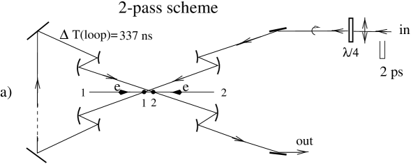
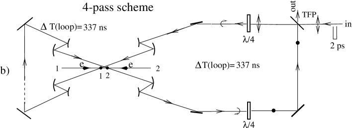
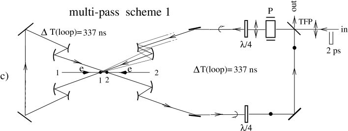
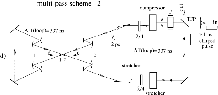
Figure 1: Optical trap: a) 2–pass optics for $e\to\gamma$ conversions; b) 4–pass optics; c) optical storage ring without stretching–compression; d) optical storage ring with stretching–compression; P is a Pockels cell, TFP is a thin film polariser, thick dots and double arrows show the direction of polarisation.

In Fig. 1a the laser pulse is used twice for the $e\to\gamma$ conversion. After the collision with the electron beam (number 1) the laser beam exits from the detector and after a 337$\,\mathrm{ns}$ loop (the interval between beam collisions at TESLA) returns back and collides with the opposite electron beam (number 2). The second pass does not need any special optical elements, only mirrors. This is a very natural and simple solution. In this scheme the laser system should generate bunches with an interval of 337$\,\mathrm{ns}$.

In Fig. 1b the laser pulse is used for conversion four times. In this scheme one additional optical element is used, a thin film polariser (TFP), which is transparent for the light polarised in the plane of the plane of the drawing and reflects light with the orthogonal polarisation. Directions of the polarisation during the first cycle are shown in Fig. 1b. After the first cycle the polarisation is perpendicular to the plane of the drawing and the light is reflected from the TFP, while after the second cycle the polarisation will be again in the plane of the drawing and the laser pulse will escape the system via the TFP. The laser bunches are emitted by the laser at an average interval of 2$\times$337$\,\mathrm{ns}$ but not uniformly (337, 3$\times$337), (337, 3$\times$337), etc (see the next paragraph).

In Fig. 1c the laser pulse is sent to the interaction region where it is trapped in an optical storage ring, which can be built using Pockels cells (P), thin film polarisers (TFP) and 1/4–wavelength plates ($\lambda/4$). Each bunch makes several ($n$) round trips (period of the round trip is $2T_{0}$, where $T_{0}=337\,\mathrm{ns}$ is the interval between bunch collisions) and then is removed from the ring. All this can be done by switching one Pockels cell which can change the direction of linear polarisation by 90 degrees. The $\lambda/4$ plates are used for obtaining the circular polarisation at the collision point. For obtaining linear polarisation at the IP these plates should be replaced by 1/2 wavelength plates. A similar kind of optical trap was considered as one of the options in the NLC Zero Design Report [22]. The number of cycles is determined by the attenuation of the pulse and by nonlinear effects in the optical elements. The latter problem is very serious for Terawatt (TW) laser pulses. During one total loop each bunch is used for conversion twice (see Fig. 1c). The laser bunch collides first with electron beam 1 travelling to the right and after a time equal to the interval between collisions (337$\,\mathrm{ns}$) it collides with beam 2 travelling to the left. For arbitrary number of the round trips, $n$, the laser pulse sequence is a sum of two uniform trains with the interval between neighbouring pulses in each train

$$\Delta T_{t}=2nT_{0}$$ (1)

and the trains are shifted by the time

$$\Delta T=kT_{0},\;\;\;\;k=1,3,\ldots 2n-1.$$ (2)

In Fig. 1d the laser pulse is trapped in the same way as in Fig. 1d, but to avoid the problems of nonlinear effects (self–focusing) in the optical elements, the laser pulse is compressed using a grating pair before collision with the electron bunch down to about $2$–$3\,\mathrm{ps}$ using grating pairs. It is then stretched again (decompressed) using another grating pair up to the previous length of about 11 ns just before passing through the optical elements.

Which system is the better one, 1b, 1c or 1d, is not clear a priori. The scheme (b) allows only 2 round trips, in the scheme (c) the number of cycles is limited by nonlinear effects, in the scheme (d) there is additional attenuation by the gratings used for compression and stretching. Optical companies suggest gratings for high powerful lasers with $R\approx 95\%$. One round trip requires four gratings, or a 20% loss/trip. So, the maximum number of trips for the scheme (d) is only about two. This presents no advantage compared to the scheme 1b which is much simpler and also allows two cycles, though it is not excluded that gratings with higher reflectivity will be available in future.

We next address the question how large the decrease of the laser energy per round trip can be in the scheme (c) without bunch compressor–stretchers. The minimum number of mirrors in the scheme is about $15$–$20$. The reflectivity of multilayer dielectric mirrors for large powers suggested by optical companies is about 99.8% (or better). The total loss/cycle is thus about $3$–$4\%$. Let us add 1% attenuation in the Pockels cell. Due to the decrease of the laser flash energy the luminosity will vary from collision to collision. Calculations show that for attenuation factors of 1.3, 1.4, 1.5 for the laser pulse , the $\gamma\gamma$ luminosity will only vary by 14, 17, 21% (here we assumed that on average the thickness of the laser target is one collision length). For 5% loss/turn and 6 round trips the attenuation is 1.35, which is still acceptable.

Let us consider the problem of nonlinear effects for the scheme 1c. The refractive index of the material depends on the beam intensity

$$n=n_{0}+n_{2}I.$$ (3)

This leads to two types of a self focusing of the laser beam [209]. The first type is a self–focusing of the beam as a whole. The second one is self–focusing and amplification of non–uniformities which leads to break up of the beam into a large number of filaments with intensities exceeding the damage level. Both these effects are characterised by the parameter “B–integral” [209, 22]

$$B=\frac{2\pi}{\lambda}\int\Delta ndl=\frac{2\pi}{\lambda}n_{2}I_{peak}\Delta l,$$ (4)

where $\Delta l$ is the thickness of the material.

If the beam has a uniform cross section then nonlinear effects do not lead to a change of the beam profile, while for the Gaussian like beam, $B\approx 1$ corresponds to the self–focusing angle approximately equal to the diffraction divergence of the beam. This is not a problem since such distortions can be easily corrected using adaptive optics (deformable mirrors).

The second effect is more severe. Even for a uniform (in average) distribution of the intensity over the aperture a small initial perturbation $\delta{I_{0}}$ grows exponentially with a rate depending on the spatial wave number. The maximum rate is given in terms of the same parameter $B$ [209]

$$\delta{I}=\delta{I}_{0}e^{B}.$$ (5)

This has been confirmed experimentally. To avoid amplification of small–scale non–uniformities, the parameter $B$ should be smaller than $3-4$ [209, 22], in other words

$$I_{peak}<\frac{\lambda}{2n_{2}\Delta l}.$$ (6)

Now we can evaluate the relationship between the diameter and the maximum thickness of the material. For $A=5\,\mathrm{J}$, $\lambda=1\,\mu\mathrm{m}$, $\sigma_{L,z}$ = 1.5$\,\mathrm{ps}$, a typical value of $n_{2}\approx 3\times 10^{-16}\,\mathrm{cm}^{2}/\,\mathrm{W}$ and a uniform beam we get

$$\Delta l[\mathrm{cm}]<0.1S[\mathrm{cm}^{2}].$$ (7)

For a beam diameter of 15$\,\mathrm{cm}$ we obtain $l<17\,\mathrm{cm}$. For Gaussian beams the maximum thickness is about two times smaller.

Next we address the question what value to insert for $\Delta l$. In the scheme 1c the dominant contribution to the total thickness is given by the Pockels cell. After the Pockels cell one can put a spatial filter (small hole in a screen) and thus suppress the growth of spikes. $\Delta l$ in this case is the thickness of the Pockels cell and does not depend on the number of round trips. Moreover, the laser pulse is very short, has a broad spectrum and the corresponding coherence length is small, about $l_{c}\approx 4\pi\sigma_{L,z}\approx 0.5\,\mathrm{cm}$. The instabilities over a uniform high intensity background develop due to the interference of the fluctuation with the main power. However, this coherence is lost after one coherence length. Thus, the B–integral does not characterise the exponential growth of small scale non-uniformities once the coherence length is much lower than $\Delta l$ (it will be suppressed even for small values of $\Delta l$, if the material is distributed over a long distance).

It turns out that the problem of nonlinear effects in the scheme 1c is not dramatic. The construction of a Pockels cells with an aperture of about $10$–$15\,\mathrm{cm}$ and a switching time of 300$\,\mathrm{ns}$ is not very difficult. Quarter– and half–wave plates can be made thin or even combined with mirrors (retarding mirror).

In conclusion, a very preliminary analysis shows that the optical scheme 1c with about 6 round trips (12 collisions with electron beams) is a very attractive and realistic solution for the TESLA photon collider.

Now a few words on the laser system required for such an optical storage ring with 6 round trips. Schematically it is shown in Fig. 2. At the start (not shown) a low–power laser produces a train of 1$\,\mathrm{ms}$ duration consisting of 500 chirped pulses with durations of several ns each. Then these pulses are distributed between 8 final amplifiers. Each of the 8 sub–trains has a duration of 1 msec and consists of 62 pulses. After amplification up to the energy of 5$\,\mathrm{J}$ in one pulse these sub–trains are recombined to reproduce the initial time structure. The time spacing between bunches in the resulting train may be equal in average (see (2)) to the 6 intervals between beam collisions in TESLA in average (see 1).

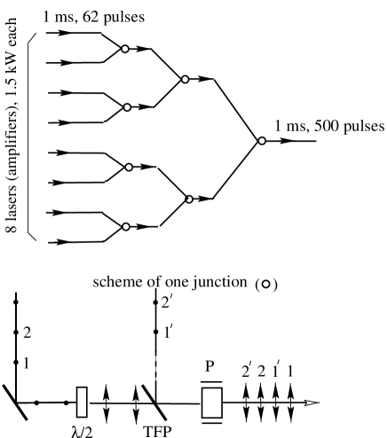
Figure 2: Merging of pulses from several lasers (amplifiers)

Due to the high average power the lasers should be based on diode pumping. Diodes have a much higher efficiency than flash lamps. It is about $\epsilon\approx 25\%$ for single pulses. For pulse trains, as in our case, the efficiency should be at least by a factor of two higher. Moreover, diodes are much more reliable. This technology has been developed very actively for other applications, such as inertial fusion.

The main problem with diodes are their cost. The present cost of diode lasers is about 5 EUR  per Watt [210]. Let us estimate the required laser power. In the case of TESLA, the duration of the pulse train T₀ = 1$\,\mathrm{ms}$ is approximately equal to the storage time ($\tau\approx 1$ msec) of the most promising powerful laser crystals, such as Yb:S-FAP. Therefore, the storage time does not help at TESLA. The required power of the diode pumping is

$$P_{diode}=\frac{A(\mbox{flash})N(\mbox{bunches})}{\epsilon T_{0}}=\frac{5\mbox{J}\times 500}{0.5\times 10^{-3}\;}=5\mbox{MW}.$$ (8)

Correspondingly, the cost of such diode system will be 25 M EUR . Here we assumed a 6–fold use of one laser bunch as described above.

Moreover, the Livermore laboratory is now working on a project of inertial confinement fusion with a high repetition rate and efficiency with the goal of building a power plant based on fusion. This project is based on diode pumped lasers. According to [211] they are currently working on the “integrated research experiment” for which “the cost of diodes should be reduced to 0.5 EUR /Watt and the cost of diodes for fusion should be 0.07 EUR /Watt or less.” Thus, the perspectives of diode pumped lasers for photon colliders are very promising. With 1 EUR /Watt the cost of diodes is 5 M EUR  for the scheme with 6 round trips (with Pockels cell) and 15 M EUR  for 2 round trips without Pockels cell.

The average output power of all lasers in the scheme 1c is about 12$\,\mathrm{kW}$, or 1.5$\,\mathrm{kW}$ for each laser.

The optical cavity

One problem with the optical storage ring at photon colliders is the self–focusing in optical elements due to the very high laser pulse power. There is another way to “create” a powerful laser pulse in the optical “trap” without any material inside: laser pulse stacking in an “external” optical cavity [9].

In short, the method is the following. Using a train of low energy laser pulses one can create in the external passive cavity (with one mirror having some small transmission) an optical pulse of the same duration but with an energy higher by a factor of $Q$ (cavity quality factor). This pulse circulates many times in the cavity each time colliding with electron bunches passing the centre of the cavity. For more details see [9].

Such kind of cavity would allow to drastically reduce the overall costs of the laser system. Instead of several parallel working lasers it could be one table–top laser feeding the external optical cavity.

A possible layout of the optics scheme at the interaction region is shown in Fig. 3 [9, 21]. In this variant, there are two optical cavities (one for each colliding electron beam) placed outside the electron beams.

Figure 3: Principle scheme of “external” cavity for $e\to\gamma$ conversion. Laser beam coming periodically from the right semi–transperant mirror MT excites one cavity (includes left–down focusing mirror, right–up focusing mirror and the MT mirror. The second cavity (for conversion of the opposite electron beam) is pumped by laser light coming from the left (not shown) and includes the focusing mirrors left–up and right–down.

Such a system has the minimum number of mirrors inside the detector. One of several possible problems in such a linear cavity is the back–reflection. In a ring type cavity this problem would be much easier to solve [212]. A possible scheme of such a ring cavity for photon colliders is shown in Fig. 4 [21] (only some elements are shown).

Figure 4: Ring type cavity. Only the cavity for one electron beam is shown. The top view is quite similar to that in Fig. 3

.

Some technical aspects of the external cavity approach are discussed in [212]. Such a cavity is operated already in MBI(Berlin) and $Q\approx 100$ has been demonstrated. A first view on technical problems of the optical cavities are given below.

The external resonant cavities have been used for comparable purposes for many years. A common application of those cavities is frequency conversion of the fundamental laser wavelength into its harmonics. Several optical laboratories have broad experience in application and design of those optical resonant enhancement cavities.

In order to provide an effective storage of the laser radiation, the length of the cavity has to be adjusted to an integer multiple of the laser wavelength with sub–micrometer accuracy. This ensures that the recirculating wave constructively interferes with the wave which is constantly fed into the cavity. An electronic feedback system is required for this task. Many different ways for obtaining the error signal are described in the scientific literature. The actual control of the resonator length is performed by means of piezoceramics which directly drive one of the resonator mirrors.

The quality factor $Q$ of the cavity is typically limited by reflection losses at the optical elements. A cavity which has been operated at the Max–Born–Institute for several years for frequency doubling reaches a quality factor of 40 without difficulties, being determined by a nonlinear crystal. After removing the nonlinear crystal, an increase of the $Q$–factor to about 100 was observed.

The majority of the cavities are used with uninterrupted cw laser radiation. Several laboratories have introduced appropriate extensions in order to use the cavities with pulses from mode locked lasers [213]. There are three major additional requirements to be fulfilled if the cavity has to store intensive laser pulses instead of cw radiation [214].

One of the problems in the optical cavity is temporal broadening of the pulse travelling in the cavity. This unfavourable effect may be caused by the wavelength dependency of the refractive index (i.e. dispersion) which is experienced by the pulse passing through the optical elements. Appropriate compensation can be done using specially designed multilayer coatings (so called ”chirped mirrors”) [215], which are now commonly used in femtosecond laser oscillators. The chirped mirrors introduce particularly small optical losses and are therefore preferable for high–$Q$ cavities. The maximum total thickness of the optical elements, whose dispersion can be compensated in one single reflection at a chirped mirror is limited to a few millimetres.

The design criteria for the resonant enhancement cavity follows:

• The cavity should have a ring–like geometry.

• The length of the cavity should be adjusted to the repetition rate of the electron bunches.

• The cavity length has to be stabilised to a very small fraction of the wavelength.

• Chirped mirrors can be used to compensate for dispersion in optical transmissive elements of up to several millimetres thickness. However, nonlinear perturbation of the wavefront by self–focusing limits this thickness to the millimetre or sub–millimetre range.

• Deformable mirrors should be used for maintaining the phase of the circulating light.

• Thin glass plates should be used for protection of individual mirrors from electrons and gamma radiation.

• The cavity cannot contain thick vacuum windows, i.e. the whole cavity has to be placed in a vacuum system.

Fig. 5 shows the basic elements of a possible resonant optical cavity for the TESLA Photon Collider (here two mirrors are missing which would allow to remove the laser beam from the IP region without passing the detector, as shown in Figs. 3, 4). The laser radiation is transferred to the cavity by means of two deformable mirrors M1 and M2. Those mirrors consist of a coated elastic glass plate which is bent by a number of piezo actuators. The purpose of the mirrors M1 and M2 is to adapt the incoming wavefront to the eigenmode to be excited in the cavity within a small fraction of the wavelength. This is essential in order to achieve constructive interference between the pulses from the laser and the pulses travelling inside the cavity. The actual coupling of the laser radiation into the cavity is performed by mirror M3 which should have a transmission of 1% (i.e. 99% reflectivity). All other mirrors M4 to M8 of the cavity are optimised for maximum reflectivity.

In order to maintain the phase of the circulating light wave across the complete beam profile, the optical path length should be adjusted locally at different positions in the beam. The required accuracy is the order of 0.1% of the wavelength. We propose to use the deformable mirrors M4 and M8 for this aim. The error signal for driving the individual piezo actuators of these mirrors may be obtained by processing the image from a CCD camera located behind the resonator mirror M3. A feedback procedure optimises the coupling of the laser radiation into the cavity and minimises the losses of the stored laser field by adjusting the actuators of M4 and M8 for minimal leakage through M3. In addition, it allows for compensation of wavefront distortions by the optical elements of the cavity and ensures that the travelling optical wave can be focused in an optimum way

The $Q$ factor of the cavity strongly depends on the reflectivity of the mirrors. Mirrors with multilayer coatings of reflectivity greater than 99.9% are already commercially available. The remaining loss in reflection of high–power mirrors is mainly caused by scattering at small impurities in the coatings. Therefore increasing the reflectivity requires to reduce the number of scattering impurities which can only be achieved by very special and expensive coating techniques.

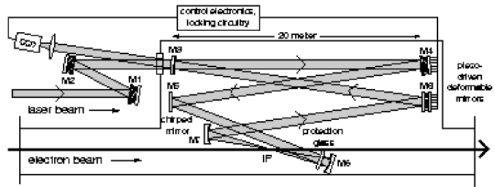
Figure 5: External ring cavity for a TESLA photon collider. See comments in the text.

A problem in the realisation of the cavity may be connected with a gradual damage of the coatings by synchrotron radiation and scattered electrons. This damage will lead to a slow reduction of the overall reflectivity of the mirrors thereby reducing the overall $Q$–factor of the cavity. The effect will be particularly important for the mirror located downstream the electron beam (M6 in Fig. 5). In order to avoid the damage we propose to protect this mirror with a thin glass plate. This plate should have antireflection coatings and easily exchangeable without misalignment of the cavity.

Taking into account these limitations we have estimated that a quality factor of $Q=100$ should be within reach. This also complies with the value obtained in already operating external cavities for cw lasers. A $Q\approx 50$ would be sufficient for the photon collider at TESLA.

Because of the high average power and the high stability, the laser has to be laid out in MOPA (Master Oscillator – Power Amplifier) geometry. Probably only diode–pumped solid–state laser systems can reach the required reproducibility of the laser parameters. The most promising candidate for a laser suitable for the TESLA Photon Collider seems to be Ytterbium–doped YAG (Yb:YAG) which has already been used to generate pulses of 0.7$\,\mathrm{ps}$ duration [216]. It has also been demonstrated that this material can deliver a very high average laser power of up to 1$\,\mathrm{kW}$ [217].

Laser damage of optics

The peak and average power in the laser system at the Photon Collider is very large. The damage threshold for multilayer dielectric mirrors depends on the pulse duration. The empirical scaling law is [209]

$$E_{th}[\mbox{J/cm}^{2}]\approx 10\sqrt{t[\mbox{ns}]}$$ (9)

for pulse durations ranging from picoseconds to milliseconds. At the LLNL the damage threshold for 1.8 ps single pulses of 0.7 to 2$\,\mathrm{J}$/cm² have been observed on commercial multilayer surfaces [22] with an average flux on the level of $3$–$5\,\mathrm{kW}$/cm².

Comparing these numbers with the conditions at the TESLA Photon Collider (5$\,\mathrm{J}$ for 1.5$\,\mathrm{ps}$, 6000$\times$5$\,\mathrm{J}$ for 1$\,\mathrm{ms}$ and 140$\,\mathrm{kW}$ average power) one finds that the average power requirements are most demanding. With a uniform distribution, the surface of the mirrors should be larger than 140/5 = 28$\,\mathrm{cm}^{2}$ and a factor of $2$–$3$ larger for Gaussian laser beams with cut tails. So, the diameter of the laser beam on mirrors and other surfaces should be larger than 10$\,\mathrm{cm}$.

Short summary on the optical schemes

We have considered two possible options of laser optics for the TESLA photon collider:

1. Optical trap (storage ring) with about 8 diode pumped driving lasers (final amplifiers) with a total average power of about 12$\,\mathrm{kW}$. Beams are merged to one train using Pockels cells and thin–film polarisers. Each laser pulse makes 6 round trips in the optical trap colliding 12 times with the electron beams. This can be done now: all technologies exist.

2. External optical cavity is a very attractive approach which can additionally reduce the cost and complexity of the laser system. This scheme requires very small tolerances (of the order of $\lambda/(2\pi Q)$, where $Q\approx 50$) and very high mirror quality. R&D is required.

2 The lasers

In this proposal we do not present a detailed scheme of a laser for the TESLA PhotonCollider. It should be an additional R&D. However, we would like to consider briefly existing laser technologies which allow, in principle, the laser system required for the Photon Colliders to be built.

Development of laser technologies is being driven by several large programs, such as inertial fusion. This is a fortunate situation for photon colliders as we may benefit from the laser technology developments of the last $10$–$15$ years which cost hundreds M$ per year. Now practically all components exist and we can just design and build the required system. Fortunately this possibility has appeared almost exactly in the time when the physics community is ready for construction of the TESLA Linear Collider. Of course, construction of the laser system for the Photon Collider is not a simple task and needs many efforts.

Two kind of lasers for photon colliders are feasible now: a solid state laser and a free electron laser (FEL).

The technology for production of picosecond pulses with terawatt power has been developed for solid state lasers. The wave length of the most powerful lasers about 1$\,\mu\mathrm{m}$ which is just optimum for the TESLA Photon Collider.

A free electron laser (FEL) is also attractive because it has a variable wave length and is based fully on the accelerator technology. The X-ray FEL with a wave length down to 1nm is a part of the TESLA project. The same technology can be used for the construction of an FEL with 1$\,\mu\mathrm{m}$ wave length for the Photon Collider. This task is much easier than the X–ray laser.

Solid state lasers

In the last decade the technique of short powerful lasers made an impressive step and has reached petawatt ($10^{15}$) power levels and few femtosecond durations [218]. Obtaining few joule pulses of picosecond duration is not a problem using modern laser techniques. For photon collider applications the main problem is the high repetition rate.

The success in obtaining picosecond pulses is connected with a chirped pulse amplification (CPA) technique [219]. “Chirped” means that the pulse has a time–frequency correlation. The main problem in obtaining short pulses is the limitation on peak power imposed by the nonlinear refractive index. This limit on intensity is about 1$\,\mathrm{GW}$/$\,\mathrm{cm}^{2}$. The CPA technique successfully overcomes this limit.

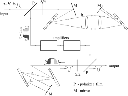
Figure 6: Chirped pulse amplification.

The principle of CPA is demonstrated in Fig. 6. A short, low energy pulse is generated in an oscillator. Then this pulse is stretched by a factor about $10^{4}$ in the grating pair which introduces a delay proportional to the frequency. This long nanosecond pulse is amplified and then compressed by another grating pair to a pulse with the initial or somewhat longer duration. As nonlinear effects are practically absent, the obtained pulses have a very good quality close to the diffraction limit.

One such laser worked since 1994 in the E–144 experiment at SLAC which studied nonlinear QED effects in the collision of laser photons with 50$\,\mathrm{GeV}$ electrons [220]. It has a repetition rate of 0.5$\,\mathrm{Hz}$, $\lambda=1.06\,\mu\mathrm{m}$ (Nd:Glass), 2$\,\mathrm{J}$ flash energy, 2$\,\mathrm{TW}$ power and 1$\,\mathrm{ps}$ duration. This is a table–top laser. Its parameters are very close to our needs, only the repetition rate was low due to overheating. In this laser a flashlamp pumping was used.

The latter problem can be solved using another very nice technique: diode pumping (the diode is a semiconductor laser with high efficiency). Since the frequency of photons from diode lasers coincides almost with the pump frequency of the 1$\,\mu\mathrm{m}$ lasers they are very efficient in converting wall plug power to laser light: efficiencies of 10% have been achieved. But even more important the heating of the laser medium with diode pumping is much lower than with flashlamps. This gives one to two orders increase in repetition rate. Moreover, the flashlamps have a limited lifetime of $<10^{6}$ shots, while the lifetime of diodes is many orders of magnitude higher.

The main problem of diodes is their cost. But it decreases very fast. As it was mentioned, their cost is 5 EUR /Watt, the next step in the inertial fusion program assumes the reduction of the cost down to 0.5 EUR /Watt and the final goal is 0.07 EUR /Watt. The cost of diodes for TESLA photon colliders would be about 25 M EUR  already with the present cost and a further significant decrease is very likely.

Below is a list of laser technologies important for photon colliders:

• chirped–pulse technique;

• diode pumping;

• laser materials with high thermo–conductivity;

• adaptive optics (deformable mirrors);

• disk amplifiers with gas (helium) cooling;

• large Pockels cells, polarisers;

• high power and high reflectivity multilayer dielectric mirrors;

• anti–reflection coatings.

Non–uniform, train structure of electron bunches at TESLA makes the task somewhat more difficult than it would be for a uniform pulse structure. This leads to rather high power of pumping diodes (high power inside one train), but as we mentioned this is not a serious problem.

However, generating a 1ms long train with 3000/6 = 500 pulses, 5$\,\mathrm{J}$ energy each, is not the same as generation of one 2.5$\,\mathrm{kJ}$ pulse (4$\,\mathrm{kJ}$ diode pumped units are developed for laser fusion) for the same time, because the volume of the laser crystal in the first case may be 500 times smaller. Beside, we consider 8 lasers working in parallel.

It is very convenient that the distance between electron bunches at TESLA is large, 337$\,\mathrm{ns}$ (1.4$\,\mathrm{ns}$ at NLC and JLC). This time allows to use large Pockels cells for manipulations of high power laser pulses.

At TESLA the train is very long and storage time of laser materials can not be used for pumping the laser medium in advance, but on the other hand, in this case, one can use a large variety of laser materials optimising other parameters (thermal conductivity etc.).

The development of the optimum design of the laser system for the Photon Collider requires special R&D. Solutions should be different for TESLA and NLC/JLC colliders.

Free electron lasers

Potential features of a free electron laser (FEL) allow one to consider it as an ideal source of primary photons for a $\gamma\gamma$ collider. Indeed, FEL radiation is tunable and has always minimal (i.e. diffraction) dispersion. The FEL radiation is completely polarised either circularly or linearly for the case of the helical or planar undulator, respectively. A driving accelerator for the FEL may be a modification of the main linear accelerator, thus providing the required time structure of laser pulses. The problem of synchronisation of the laser and electron bunches at the conversion region is solved by means of traditional methods used in accelerator techniques. A FEL amplifier has the potential to provide a high conversion efficiency of the kinetic energy of the electron beam into coherent radiation. At sufficient peak power of the driving electron beam the peak power of the FEL radiation could reach the required TW level.

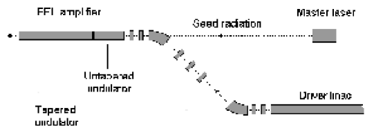
Figure 7: Basic scheme of the MOPA laser system for a photon collider.

The idea to use a FEL as a laser for the $\gamma\gamma$ collider has been proposed in [221]. The present view on FEL systems for the photon collisions at TESLA is discussed in [222]. The FEL system is built as a master oscillator–power amplifier (MOPA) scheme where the low–power radiation from a Nd glass laser ($\lambda=1\,\mu\mathrm{m}$) is amplified in a long tapered undulator by an electron beam (see Fig. 7). The driving accelerator has the same pulse structure as the main TESLA linac.

The driving electron beam for the FEL is produced by the accelerator based on TESLA technology and similar to the TTF (TESLA Test Facility) accelerator [223]. Parameters of the accelerator are presented in Table 1. The beam with a charge of 12$\,\mathrm{nC}$ and normalised emittance of 30$\pi\,\,\mathrm{mm}\,\,\mathrm{mrad}$ is generated in the photoinjector, accelerated in superconducting modules with the gradient $20-25\mbox{MV}/\,\mathrm{m}$ and compressed down to a 2$\,\mathrm{ps}$ duration in the bunch compressors. Note that the emittance is not a critical parameter for the considered FEL. The number of bunches per macropulse is about 3 times lower than that in the TESLA train, but as discussed in the previous section one laser bunch can be used several times for $e\to\gamma$ conversion.

Energy	1.5$\,\mathrm{GeV}$
Charge per bunch	12$\,\mathrm{nC}$
Peak current	2.4$\,\mathrm{kA}$
Bunch length (RMS)	0.6$\,\mathrm{mm}$
Normalised emittance	30$\pi\,\mathrm{mm}\,\mathrm{mrad}$
Energy spread (RMS)	1$\,\mathrm{MeV}$
Repetition rate	5$H^{0}$
Macropulse duration	800$\,\mu\mathrm{s}$
# of bunches per macropulse	1130
Bunch spacing	708$\,\mathrm{ns}$
Average beam power	102$\,\mathrm{kW}$

Table 1: Parameters of the driving accelerator

Undulator
Type	Helical
Period	10$\,\mathrm{cm}$
Magnetic field (entr./exit)	1.4$\,\mathrm{T}$/ 1.08$\,\mathrm{T}$
Total length	60$\,\mathrm{m}$
Length of untapered section	10.7$\,\mathrm{m}$
Beam size in the und. (RMS)	230$\,\mu\mathrm{m}$
Radiation
Wavelength	1$\,\mu\mathrm{m}$
Dispersion	Dif. limit
Pulse energy	2.2$\,\mathrm{J}$
Pulse duration (HWHM)	1.6$\,\mathrm{ps}$
Repetition rate	5$\,\mathrm{Hz}$
Macropulse duration	800$\,\mu\mathrm{s}$
# of pulses per macropulse	1130
Peak output power	0.7$\,\mathrm{TW}$
Average power	12.5$\,\mathrm{kW}$
Efficiency	12.2%

Table 2: Parameters of the FEL amplifier

The peak power of the master laser with the wavelength of 1$\,\mu\mathrm{m}$ is assumed to be $1m_{\mathrm{W}}$ with a pulse duration of several picoseconds, so that the average power will be below 0.1$\,\mathrm{W}$. This means that only a small fraction of the power can be taken from the 2$\,\mathrm{W}$ of infrared radiation generated in the laser system of the photoinjector. Then this radiation can be transported to the undulator entrance. The problem of synchronisation of electron and optical bunches is therefore solved naturally.

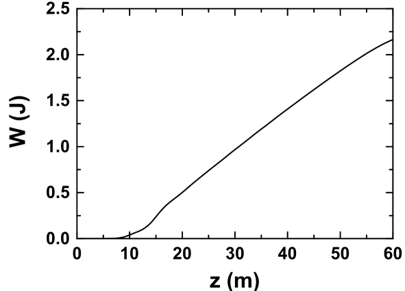
Figure 8: Energy in the radiation pulse versus the undulator length.

To obtain reasonable luminosity of the $\gamma\gamma$ collider at TESLA, the energy in the radiation pulse at the FEL amplifier exit should be above 2$\,\mathrm{J}$ and the peak power should reach sub–terawatt level. For the chosen parameters of the electron beam this means that the FEL efficiency must exceed 10%. In an FEL amplifier with a uniform undulator the efficiency is limited by saturation effects and is below 1% in the considered case. Saturation of the radiation power in the FEL amplifier occurs due to the energy loss by the particles which fall out of the resonance with the electromagnetic wave. Nevertheless, effective amplification of the radiation is possible in the nonlinear regime by means of using a tapered undulator. In this case a large fraction of particles is trapped in the effective potential of the interaction with the electromagnetic wave and is decelerated.

Parameters of the FEL amplifier with the tapered undulator are presented in Table 2. The tapering can be done by decreasing the magnetic field at fixed undulator period. The undulator is helical to provide polarised radiation and is superconducting. The resonance is maintained by decreasing the magnetic field at fixed period of the undulator.

The dependence of the radiated energy versus the undulator length is shown in Fig. 8. The efficiency 12.2%, reached in the end of the undulator, corresponds to 2.2$\,\mathrm{J}$ in the optical pulse.

Use of a free electron laser as a source of primary photons for the $\gamma\gamma$ collider at TESLA seems to be natural solution. TESLA already includes an integrated X–ray FEL facility. Powerful VUV radiation has been produced at DESY in a SASE FEL with 15$\,\mathrm{m}$long undulator [224]. The FEL for the photon colliders is simpler than the X–ray FEL.

Scale and cost of the FEL facility for the Photon Collider can be estimated in a simple way. It requires a 1.5$\,\mathrm{GeV}$ linear accelerator similar to the main TESLA accelerator and a 60$\,\mathrm{m}$ long undulator.

Summary on lasers

We have considered briefly two kinds of lasers for the photon collider at TESLA: a solid state laser and a FEL. Both approaches are technically feasible. However, the first one looks somewhat more attractive, because it might be a large room–size system, while a FEL includes a 160$\,\mathrm{m}$ long accelerator (with wiggler) which would be a large facility. For energies $2E_{0}\geq 800\,\mathrm{GeV}$ where longer laser wave length will be required, a FEL may be the best choice.

6 Summary

The Photon Collider presents a unique opportunity to study $\gamma\gamma$ and $\gamma e$ interactions at high energies and luminosities, which can considerably enrich the physics program of the $e^{+}e^{-}$ linear collider TESLA. The parameters of the super–conducting collider TESLA: the energy, the interval between electron bunches are particularly suited for design and performance of the Photon Collider.

This novel option requires only one new additional element: the powerful laser, which can be built using modern laser technologies. The optimum laser wave length for TESLA is about 1$\,\mu\mathrm{m}$, which is exactly the region of the most powerful developed solid state lasers.

The second interaction region and the detector may be very similar to those for $e^{+}e^{-}$ collisions and can be also be used for study of $e^{-}e^{-}$ or $e^{+}e^{-}$ interactions.

References

- [1] I. F. Ginzburg, G. L. Kotkin, V. G. Serbo, and V. I. Telnov. Pizma ZhETF, 34:514, 1981. JETP Lett. 34:491, 1982. Preprint INP 81-50, Novosibirsk, 1981.
- [2] I. F. Ginzburg, G. L. Kotkin, V. G. Serbo, and V. I. Telnov. Nucl. Instrum. Meth., 205:47, 1983. Preprint INP 81-102, Novosibirsk, 1981.
- [3] I. F. Ginzburg, G. L. Kotkin, S. L. Panfil, V. G. Serbo, and V. I. Telnov. Nucl. Instrum. Meth., A219:5–24, 1984.
- [4] V. I. Telnov. Nucl. Instrum. Meth., A294:72–92, 1990.
- [5] V. I. Telnov. Nucl. Instrum. Meth., A355:3, 1995.
- [6] M. Baillargeon, et al. In P. Zerwas (ed.), e+e- Collisions at TeV Energies: The Physics Potential, Part D, DESY 96-123D. DESY, 1995.
- [7] I. Ginzburg and V. Serbo. In Proc. of Winter School of LINP, vol. 2, p. 132, 1988.
- [8] I. F. Ginzburg. Physical Potential of Photon-Photon and Electron - Photon Colliders in TeV Region. In D. Caldwell and H. Paar (eds.), Proc. IX Intern. Workshop on Photon – Photon Collisions, San Diego, CA, USA, p. 474, 1992. World Scientific.
- [9] V. I. Telnov. In Proc. of International Conference on the Structure and Interactions of the Photon (Photon 99), Freiburg, Germany, 2000. Nucl. Phys. Proc. Suppl. 82. hep-ex/9908005.
- [10] V. Telnov. Int. J. Mod. Phys., A13:2399–2410, 1998. hep-ex/9802003.
- [11] A. N. Skrinsky. Sov. Phys. Usp., 25:639–661, 1982.
- [12] V. I. Telnov. , Collision at Linear Colliders. In Physics and Experiments with Linear Colliders, Saariselka, Finland, 1992. Ed. R. Orava et al., World Scientific.
- [13] D. L. Borden, D. Bauer, and D. O. Caldwell. Phys. Rev., D48:4018–4028, 1993.
- [14] V. I. Telnov. , at Linear Colliders. In D. Caldwell and H. Paar (eds.), Proc. IX Intern. Workshop on Photon – Photon Collisions, San Diego, CA, USA, p. 369, 1992. World Scientific.
- [15] S. J. Brodsky and P. M. Zerwas. Nucl. Instrum. Meth., A355:19–41, 1995. hep-ph/9407362.
- [16] M. Baillargeon, G. Belanger, and F. Boudjema. Electroweak Physics Issues at a High-Energy Photon Collider. 1994. hep-ph/9405359.
- [17] D. J. Miller. Other Options: , and Physics at a Linear Collider. In 3rd Workshop on Physics and Experiments with Linear Colliders (LCWS 95), Iwate, Japan, p. 305, 1995.
- [18] I. Watanabe, et al. Collider as an Option of JLC. KEK-REPORT-97-17.
- [19] R. Brinkmann et al. Nucl. Instrum. Meth., A406:13, 1998. hep-ex/9707017.
- [20] A. M. Sessler. Phys. Today, 51:48–53, 1998.
- [21] V. Telnov. Photon Collider at TESLA. In Intern. Workshop on High-Energy Photon Colliders, Hamburg, Germany, 2000. submitted to Nucl. Instrum. Meth. A. hep-ex/0010033.
- [22] The NLC Design Group. Zeroth-Order Design Report for the NLC. LBNL-5424, SLAC-474, UCBL-ID-124161, UC-414. SLAC, http://www-project.slac.stanford.edu/lc/ZDR/, 1996.
- [23] R. Brinkmann, G. Materlik, J. Rossbach, and A. Wagner (eds.). Conceptual Design of a 500 GeV e+e- Linear Collider with Integrated X-Ray Laser Facility. DESY 1997-048, ECFA 1997-182. DESY, 1997.
- [24] N. Akasaka et al. JLC Design Study. KEK-REPORT-97-1.
- [25] Nucl. Instrum. Meth., A355, 1995. Proc. of Workshop on Colliders. Berkeley CA, USA, 1994.
- [26] International Workshop On High-Energy Photon Colliders (GG 2000), Hamburg, Germany, 2000. To be published in Nucl. Instrum. Meth. A, http://www.desy.de/~gg2000/.
- [27] I. Ginzburg. In Proc. of International Conference on the Structure and Interactions of the Photon (Photon 99), Freiburg, Germany, 23-27 May 1999, 2000. Nucl. Phys. Proc. Suppl. 82:367. hep-ex/9907549.
- [28] B. Pietrzyk. The Global Fit to Electroweak Data. In Proc. International Conference on High-Energy Physics (ICHEP 2000), Osaka, Japan, 2000. LAPP-EXP-2000-06.
- [29] P. Igo-Kemenes. For the LEP Working Group on Higgs boson search, talk at the LEPC open session on Nov. 3rd, 2000, http://lephiggs.web.cern.ch/LEPHIGGS/talks/index.html.
- [30] ALEPH-Collaboration: R. Barate et al. Phys. Lett., B495:1–17, 2000. hep-ex/0011045.
- [31] L3-Collaboration: M. Acciarri et al. Phys. Lett., B495:18–25, 2000. hep-ex/0011043.
- [32] S. Heinemeyer, W. Hollik, and G. Weiglein. Eur. Phys. J., C9:343, 1999. hep-ph/9812472.
- [33] H. E. Haber. How well can we predict the Mass of the Higgs Boson of the Minimal Supersymmetric Model? In Proceedings of 4th International Symposium on Radiative Corrections (RADCOR 98): Applications of Quantum Field Theory to Phenomenology, Barcelona, Spain, 1999. hep-ph/9901365.
- [34] T. Barklow. In Research Directions for the Decade. Proceedings, Summer Study on High-Energy Physics, Snowmass, USA, p.440, 1990.
- [35] J. F. Gunion and H. E. Haber. In Research Directions for the Decade. Proceedings, Summer Study on High-Energy Physics, Snowmass, USA, p. 206, 1990.
- [36] J. F. Gunion and H. E. Haber. Phys. Rev., D48:5109–5120, 1993.
- [37] D. L. Borden, D. A. Bauer, and D. O. Caldwell. Phys. Rev., D48:4018–4028, 1993.
- [38] T. Ohgaki. Int. J. Mod. Phys., A15:2587, 2000. physics/0002020.
- [39] V. I. Telnov. Gamma Gamma, Gamma Electron Colliders. In 17th International Conference on High-Energy Accelerators (HEACC 98), Dubna, Russia, p. 98, 1998. hep-ex/9810019.
- [40] J. F. Gunion, L. Poggioli, R. V. Kooten, C. Kao, and P. Rowson. Higgs Boson Discovery and Properties. In 1996 DPF / DPB Summer Study on New Directions for High-Energy Physics (Snowmass 96), Snowmass, CO, USA, 1996. hep-ph/9703330.
- [41] H. E. Haber. Challenges for Non-Minimal Higgs Searches at Future Colliders. In Beyond the Standard Model Conf., Lake Tahoe, CA, Dec 13-18, 1994 and Ringsberg Workshop on Perspectives for Electroweak Interactions in e+ e- Collisions, Ringsberg, Germany, 5-8 Feb 1995., 1995. Published in Ringsberg Electroweak 1995:219-232. hep-ph/9505240.
- [42] A. Djouadi, V. Driesen, W. Hollik, and J. I. Illana. Eur. Phys. J., C1:149–162, 1998. hep-ph/9612362.
- [43] B. Grzadkowski and J. F. Gunion. Phys. Lett., B294:361–368, 1992. hep-ph/9206262.
- [44] J. F. Gunion and J. G. Kelly. Phys. Lett., B333:110–117, 1994. hep-ph/9404343.
- [45] M. Krämer, J. Kühn, M. L. Stong, and P. M. Zerwas. Z. Phys., C64:21–30, 1994. hep-ph/9404280.
- [46] S. Söldner-Rembold and G. Jikia. Light Higgs production at a Photon Collider. In Intern. Workshop on High-Energy Photon Colliders, Hamburg, Germany, 2000. submitted to Nucl. Instrum. Meth. A. See [26].
- [47] M. Melles, W. J. Stirling, and V. A. Khoze. Phys. Rev., D61:054015, 2000. hep-ph/9907238.
- [48] T. Ohgaki, T. Takahashi, and I. Watanabe. Phys. Rev., D56:1723–1729, 1997. hep-ph/9703301.
- [49] T. Ohgaki, T. Takahashi, I. Watanabe, and T. Tauchi. Int. J. Mod. Phys., A13:2411, 1998.
- [50] M. Melles. Precision Higgs Physics at a Collider. In Intern. Workshop on High-Energy Photon Colliders, Hamburg, Germany, 2000. submitted to Nucl. Instrum. Meth. A. hep-ph/0008125.
- [51] M. Melles. In International Conference on the Structure and Interactions of the Photon (Photon 99), Freiburg, Germany and 4th International Workshop on Linear Colliders (LCWS 99), Sitges, Spain, p. 379, 2000. Nucl. Phys. Proc. Suppl. 82. hep-ph/9906467.
- [52] K. A. Ispirian, I. A. Nagorskaya, A. G. Oganesian, and V. A. Khoze. Yad. Fiz., 11:1278–1283, 1970.
- [53] K. A. Ispirian, I. A. Nagorskaya, A. G. Oganesian, and V. A. Khoze. Sov. J. Nucl. Phys., 11:712, 1970.
- [54] G. Jikia and S. Söldner-Rembold. Nucl. Phys. Proc. Suppl., 82:373–378, 2000. hep-ph/9910366.
- [55] G. Jikia and A. Tkabladze. Nucl. Instrum. Meth., A355:81–83, 1995. hep-ph/9406428.
- [56] G. Jikia and A. Tkabladze. Phys. Rev., D54:2030–2042, 1996. hep-ph/9601384.
- [57] D. L. Borden, V. A. Khoze, W. J. Stirling, and J. Ohnemus. Phys. Rev., D50:4499–4507, 1994. hep-ph/9405401.
- [58] V. A. Khoze. On Measuring the Gamma Gamma Width of the Intermediate Mass Higgs at a Photon Linear Collider. In Photon ’95. 10th International Workshop on Gamma Gamma Collisions and Related Processes, Sheffield, UK, p. 392, 1995. World Scientific, Singapore. hep-ph/9504348.
- [59] M. Melles and W. J. Stirling. Nucl. Phys., B564:325–342, 2000. hep-ph/9903507.
- [60] M. Melles and W. J. Stirling. Eur. Phys. J., C9:101–106, 1999. hep-ph/9810432.
- [61] M. Melles and W. J. Stirling. Phys. Rev., D59:094009, 1999. hep-ph/9807332.
- [62] M. Battaglia. Measuring Higgs Branching Ratios and Telling the SM from a MSSM Higgs Boson at the e+ e- Linear Collider. In E. Fernández and A. Pacheco (eds.), Proceedings of the Worldwide Study on Physics and Experiments with Future Linear Colliders, p. 163, Sitges, Spain, 1999. Universitat Autònoma de Barcelona. hep-ph/9910271.
- [63] D. A. Morris, T. N. Truong, and D. Zappala. Phys. Lett., B323:421–426, 1994. hep-ph/9310244.
- [64] I. F. Ginzburg and I. P. Ivanov. Phys. Lett., B408:325–330, 1997. hep-ph/9704220.
- [65] E. Boos, et al. Phys. Lett., B427:189–196, 1998. hep-ph/9801359.
- [66] E. Boos, et al. Higgs to WW* in Gamma Gamma Collisions. In E. Fernández and A. Pacheco (eds.), Proceedings of the Worldwide Study on Physics and Experiments with Future Linear Colliders, vol. I, p. 498, Sitges, Spain, 1999. Universitat Autònoma de Barcelona.
- [67] G. V. Jikia. Phys. Lett., B298:224–229, 1993.
- [68] G. Jikia. Nucl. Phys., B405:24–54, 1993.
- [69] M. S. Berger. Phys. Rev., D48:5121–5126, 1993. hep-ph/9307259.
- [70] D. A. Dicus and C. Kao. Phys. Rev., D49:1265–1271, 1994. hep-ph/9308330.
- [71] E. Boos, J. C. Brient, D. W. Reid, H. J. Schreiber, and R. Shanidze. Measuring the Higgs Branching Fraction into Two Photons at Future Linear Colliders. 2000. hep-ph/0011366.
- [72] D. W. Reid. Measurement of the Branching Ratio B(H). In E. Fernández and A. Pacheco (eds.), Proceedings of the Worldwide Study on Physics and Experiments with Future Linear Colliders, vol. I, p. 179, Sitges, Spain, 1999. Universitat Autònoma de Barcelona.
- [73] M. M. Mühlleitner. Production of MSSM Higgs Bosons in Gamma-Gamma Collisions. In Intern. Workshop on High-Energy Photon Colliders, Hamburg, Germany, 2000. submitted to Nucl. Instrum. Meth. A. See [26].
- [74] M. M. Mühlleitner, M. Krämer, M. Spira, and P. M. Zerwas. Production of MSSM Higgs bosons in photon photon collisions. 2001. hep-ph/0101083.
- [75] ATLAS Collaboration. ATLAS: Detector and Physics Performance Technical Design Report. CERN, LHCC 99-14, 1999. http://atlasinfo.cern.ch/Atlas/GROUPS/PHYSICS/TDR/access.html.
- [76] CMS Collaboration. The Compact Muon Solenoid, Technical Proposal. CERN, LHCC 94-38, 1994. http://cmsinfo.cern.ch/TP/TP.html.
- [77] A. Djouadi, J. Kalinowski, P. Ohmann, and P. M. Zerwas. Z. Phys., C74:93–111, 1997. hep-ph/9605339.
- [78] ECFA/DESY LC Physics Working Group-Collaboration: E. Accomando et al. Phys. Rept., 299:1–78, 1998. hep-ph/9705442.
- [79] P. M. Zerwas. Physics with an Linear Collider at High Luminosity. In B. B. Levchenko and V. I. Savrin (eds.), 14th International Workshop On High Energy Physics And Quantum Field Theory, Moscow, Russia, 2000. hep-ph/0003221.
- [80] M. M. Mühlleitner. Higgs Particles in the Standard Model and Supersymmetric Theories. Ph.D. thesis, 2000. hep-ph/0008127.
- [81] C. N. Yang. Phys. Rev., 77:242–245, 1950.
- [82] S. Y. Choi and K. Hagiwara. Phys. Lett., B359:369–374, 1995. hep-ph/9506430.
- [83] J. I. Illana. Resonant Production of Heavy MSSM Higgs Bosons at the Photon Collider. In 4th Workshop on Physics and Detectors for a Linear Electron Positron Collider (2nd Joint ECFA / DESY Study), Oxford, England, 1999. hep-ph/9912467.
- [84] I. F. Ginzburg and I. P. Ivanov. CP Odd Anomalous Interactions of Higgs Boson in its Production at Photon Colliders. 2000. hep-ph/0004069.
- [85] E. Asakawa. Heavy Higgs Productions at Gamma Gamma Colliders. In E. Fernández and A. Pacheco (eds.), Proceedings of the Worldwide Study on Physics and Experiments with Future Linear Colliders, Sitges, Spain, 1999. Universitat Autònoma de Barcelona. hep-ph/9908457.
- [86] E. Asakawa, J. Kamoshita, A. Sugamoto, and I. Watanabe. Eur. Phys. J., C14:335–345, 2000. hep-ph/9912373.
- [87] I. F. Ginzburg, M. Krawczyk, and P. Osland. Potential of Photon Colliders in Resolving SM-like Scenarios. In Intern. Workshop on High-Energy Photon Colliders, Hamburg, Germany, 2000. submitted to Nucl. Instrum. Meth. A. See [26].
- [88] I. . Ginzburg, M. Krawczyk, and P. Osland. In Linear Collider Workshop, FNAL, Batavia, IL, USA, 2000. American Institute of Physics. To be published, see http://www-lc.fnal.gov/lcws2000.
- [89] E. Asakawa, S. Y. Choi, K. Hagiwara, and J. S. Lee. Phys. Rev., D62:115005, 2000. hep-ph/0005313.
- [90] M. Klasen. Sfermion Production at Photon Colliders. In Intern. Workshop on High-Energy Photon Colliders, Hamburg, Germany, 2000. submitted to Nucl. Instrum. Meth. A. hep-ph/0008082.
- [91] T. Mayer and H. Fraas. Chargino Production and Decay in Photon-Photon-Collisions. In Intern. Workshop on High-Energy Photon Colliders, Hamburg, Germany, 2000. submitted to Nucl. Instrum. Meth. A. hep-ph/0009048.
- [92] F. Cuypers, G. J. van Oldenborgh, and R. Rückl. Nucl. Phys., B383:45–57, 1992. hep-ph/9205209.
- [93] F. Cuypers, G. J. van Oldenborgh, and R. Rückl. Nucl. Phys., B409:144–160, 1993. hep-ph/9302302.
- [94] F. Cuypers. Phys. Rev., D49:3075–3078, 1994. hep-ph/9310327.
- [95] A. Goto and T. Kon. Europhys. Lett., 19:575–580, 1992.
- [96] T. Kon and A. Goto. Phys. Lett., B295:324–329, 1992.
- [97] C. Blöchinger, F. Franke, and H. Fraas. Distinguishing between MSSM and NMSSM with e Gamma Scattering. In Intern. Workshop on High-Energy Photon Colliders, Hamburg, Germany, 2000. submitted to Nucl. Instrum. Meth. A. hep-ph/0008167.
- [98] C. Blöchinger and H. Fraas. Possible test of the GUT relation between M1 and M2 in Electron-Photon scattering. LC-TH-2000-017.
- [99] D. S. Gorbunov, V. A. Ilyin, and V. I. Telnov. TESLA: Potentials of Gamma Gamma and Options in Stoponium Searches. In Intern. Workshop on High-Energy Photon Colliders, Hamburg, Germany, 2000. submitted to Nucl. Instrum. Meth. A. hep-ph/0012175.
- [100] N. Arkani-Hamed, S. Dimopoulos, and G. Dvali. Phys. Lett., B429:263–272, 1998. hep-ph/9803315.
- [101] N. Arkani-Hamed, S. Dimopoulos, and G. Dvali. Phys. Rev., D59:086004, 1999. hep-ph/9807344.
- [102] I. Antoniadis, N. Arkani-Hamed, S. Dimopoulos, and G. Dvali. Phys. Lett., B436:257–263, 1998. hep-ph/9804398.
- [103] G. F. Giudice, R. Rattazzi, and J. D. Wells. Nucl. Phys., B544:3–38, 1999. hep-ph/9811291.
- [104] T. Han, J. D. Lykken, and R.-J. Zhang. Phys. Rev., D59:105006, 1999. hep-ph/9811350.
- [105] E. A. Mirabelli, M. Perelstein, and M. E. Peskin. Phys. Rev. Lett., 82:2236–2239, 1999. hep-ph/9811337.
- [106] J. L. Hewett. Phys. Rev. Lett., 82:4765–4768, 1999. hep-ph/9811356.
- [107] T. G. Rizzo. Indirect Collider Tests for Large Extra Dimensions. In H. Klapdor-Kleingrothaus and I. Krivosheina (eds.), 2nd International Conference Physics Beyond the Standard Model: Beyond the Desert 99: Accelerator, Nonaccelerator and Space Approaches, Bristol, England, 1999. IOP. hep-ph/9910255.
- [108] T. G. Rizzo. New Physics Beyond the Standard Model at Gamma Gamma Colliders. In Intern. Workshop on High-Energy Photon Colliders, Hamburg, Germany, 2000. submitted to Nucl. Instrum. Meth. A. hep-ph/0008037.
- [109] T. G. Rizzo. Phys. Rev., D60:115010, 1999. hep-ph/9904380.
- [110] K. Cheung. Phys. Rev., D61:015005, 2000. hep-ph/9904266.
- [111] H. Davoudiasl. Int. J. Mod. Phys., A15:2613, 2000. hep-ph/0001248.
- [112] I. F. Ginzburg, G. L. Kotkin, S. L. Panfil, and V. G. Serbo. Nucl. Phys., B228:285, 1983.
- [113] I. F. Ginzburg, G. L. Kotkin, S. L. Panfil, and V. G. Serbo. Nucl. Phys., B243:550, 1984.
- [114] T. Takahashi. In Workshop on Physics and Experiments with Linear Colliders, Marioka-Appi, Japan, p. 681, 1996. World Scientific.
- [115] I. F. Ginzburg. In F. Harris, S. Olsen, S. Pakvasa, and X. Tata (eds.), Physics and Experiments with Linear Colliders, Waikoloa, USA, vol. v. II, p. 739, 1993. World Scientific.
- [116] I. F. Ginzburg, V. A. Ilyin, A. E. Pukhov, V. G. Serbo, and S. A. Shichanin. Phys. Atom. Nucl., 56:1481–1486, 1993.
- [117] I. F. Ginzburg. Nucl. Instrum. Meth., A355:63–74, 1995.
- [118] I. F. Ginzburg. Why Photon Colliders are Necessary in a Future Collider Program. In Intern. Workshop on High-Energy Photon Colliders, Hamburg, Germany, 2000. submitted to Nucl. Instrum. Meth. A. hep-ph/0101029.
- [119] M. Baillargeon, G. Belanger, and F. Boudjema. Nucl. Phys., B500:224, 1997. hep-ph/9701372.
- [120] F. Boudjema. In Workshop on Collisions at 500 GeV: The Physics Potential, 1992.
- [121] M. Baillargeon, G. Belanger, and F. Boudjema. Electroweak Physics Issues at a High-Energy Photon Collider. 1994. hep-ph/9405359.
- [122] S. J. Brodsky. Photon-Photon Collisions at the Next Linear Collider: Theory. In F. A. Harris, S. Olsen, S. Pakvasa, and X. Tata (eds.), Physics and Experiments with Linear Colliders, Waikoloa, HI, USA, p. 295, 1993. World Scientific.
- [123] G. Jikia. Nucl. Instrum. Meth., A355:84–88, 1995. hep-ph/9406395.
- [124] G. Jikia. Nucl. Phys., B437:520–540, 1995. hep-ph/9407393.
- [125] K. Cheung. Phys. Lett., B323:85–89, 1994. hep-ph/9310340.
- [126] K. Cheung. Phys. Rev., D50:4290–4298, 1994. hep-ph/9406228.
- [127] R. D. Peccei and X. Zhang. Nucl. Phys., B337:269–283, 1990.
- [128] R. D. Peccei, S. Peris, and X. Zhang. Nucl. Phys., B349:305–322, 1991.
- [129] J. L. Hewett. Int. J. Mod. Phys., A13:2389–2398, 1998. hep-ph/9803369.
- [130] E. E. Boos. Top Quarks at Photon Colliders. In Intern. Workshop on High-Energy Photon Colliders, Hamburg, Germany, 2000. submitted to Nucl. Instrum. Meth. A. hep-ph/0009100.
- [131] A. Djouadi, J. Ng, and T. G. Rizzo. New Particles and Interactions. In T. Barklow, S. Dawson, H. Haber, and J. Seigrist (eds.), Electroweak Symmetry Breaking and Beyond the Standard Model, 1995. World Scientific. hep-ph/9504210.
- [132] P. Poulose and S. D. Rindani. Phys. Lett., B452:347–354, 1999. hep-ph/9809203.
- [133] S. Y. Choi and K. Hagiwara. Phys. Lett., B359:369–374, 1995. hep-ph/9506430.
- [134] M. S. Baek, S. Y. Choi, and C. S. Kim. Phys. Rev., D56:6835–6855, 1997. hep-ph/9704312.
- [135] E. Boos, M. Dubinin, A. Pukhov, M. Sachwitz, and H. J. Schreiber. In preparation.
- [136] G. V. Jikia. Nucl. Phys., B374:83–98, 1992.
- [137] E. Yehudai, S. Godfrey, and K. A. Peterson. Single Top Production in e Gamma Collisions. In F. Harris, S. Olsen, S. Pakvasa, and X. Tata (eds.), Physics and Experiments with Linear Colliders, Waikoloa, HI, USA, 1993. World Scientific. hep-ph/9308281.
- [138] E. Boos, A. Pukhov, M. Sachwitz, and H. J. Schreiber. Single Top and Light Higgs at TeV Energy Gamma e Colliders. In 4th Workshop on Physics and Detectors for a Linear Electron Positron Collider (1st Joint ECFA / DESY Study), Hamburg, Germany, 1996. hep-ph/9711253.
- [139] E. Boos, A. Pukhov, M. Sachwitz, and H. J. Schreiber. Phys. Lett., B404:119–123, 1997. hep-ph/9704259.
- [140] J.-J. Cao, J.-X. Wang, J. M. Yang, B.-L. Young, and X.-M. Zhang. Phys. Rev., D58:094004, 1998. hep-ph/9804343.
- [141] E. Boos, L. Dudko, and T. Ohl. Eur. Phys. J., C11:473–484, 1999. hep-ph/9903215.
- [142] E. Boos, M. Dubinin, M. Sachwitz, and H. J. Schreiber. Eur. Phys. .J, C16:269–278, 2000. hep-ph/0001048.
- [143] R. Godbole and G. Pancheri. Gamma-Gamma Cross Section at Gamma-Gamma Colliders. In Intern. Workshop on High-Energy Photon Colliders, Hamburg, Germany, 2000. submitted to Nucl. Instrum. Meth. A. hep-ph/0101320.
- [144] I. F. Ginzburg, S. L. Panfil, and V. G. Serbo. Nucl. Phys., B284:685–705, 1987.
- [145] I. F. Ginzburg, S. L. Panfil, and V. G. Serbo. Nucl. Phys., B296:569–581, 1988.
- [146] I. F. Ginzburg, D. Y. Ivanov, and V. G. Serbo. Phys. Atom. Nucl., 56:1474–1480, 1993.
- [147] A. Vogt. Nucl. Phys. Proc. Suppl., 82:394–399, 2000. hep-ph/9908315.
- [148] A. Gehrmann-De Ridder, H. Spiesberger, and P. M. Zerwas. Phys. Lett., B469:259–262, 1999. hep-ph/9909230.
- [149] P. Aurenche et al. Prog. Theor. Phys., 92:175–188, 1994. hep-ph/9401269.
- [150] M. Klasen, T. Kleinwort, and G. Kramer. Eur. Phys. J. Direct, C1:1–105, 1998. hep-ph/9712256.
- [151] M. Drees, M. Krämer, J. Zunft, and P. M. Zerwas. Phys. Lett., B306:371–378, 1993.
- [152] T. Wengler and A. D. Roeck. The Gluon Content of the Photon from Di-Jet Production at the Photon Photon Collider. In Intern. Workshop on High-Energy Photon Colliders, Hamburg, Germany, 2000. submitted to Nucl. Instrum. Meth. A. hep-ph/0010293.
- [153] P. Jankowski, M. Krawczyk, and A. D. Roeck. Charm Production at a Linear and Photon Collider and its Sensitivity to the Gluon Content of the Photon. In Intern. Workshop on High-Energy Photon Colliders, Hamburg, Germany, 2000. submitted to Nucl. Instrum. Meth. A. See [26].
- [154] M. Stratmann and W. Vogelsang. Phys. Lett., B386:370–378, 1996. hep-ph/9606346.
- [155] M. Stratmann. Nucl. Phys. Proc. Suppl., 82:400–406, 2000. hep-ph/9907467.
- [156] M. Stratmann. Determining the Spin Structure of the Photon at Future Colliders. 2000. hep-ph/0006285.
- [157] J. Kwiecinski and B. Ziaja. QCD Predictions for Spin Dependent Photonic Structure Function g1(gamma)(x,Q2) in the Low x Region of Future Linear Colliders. 2000. hep-ph/0006292.
- [158] J. Kwiecinski and B. Ziaja. QCD Predictions for the Spin Dependent Structure Function g1(gamma)(x,Q2) of the Photon in the Low x Region of Colliders. In Intern. Workshop on High-Energy Photon Colliders, Hamburg, Germany, 2000. submitted to Nucl. Instrum. Meth. A. See [26].
- [159] J. Kwiecinski and L. Motyka. Phys. Lett., B438:203–210, 1998. hep-ph/9806260.
- [160] J. Kwiecinski, L. Motyka, and A. D. Roeck. The QCD Pomeron at TESLA: Motivation and Exclusive Production. In 5th Workshop on Physics and Detectors for a Linear Electron Positron Collider (2nd Joint ECFA / DESY Study), Obernai, France, 1999. hep-ph/0001180.
- [161] J. Blümlein and A. Kryukov. In Intern. Workshop on High-Energy Photon Colliders, Hamburg, Germany, 2000. submitted to Nucl. Instrum. Meth. A. hep-ph/0008097.
- [162] A. F. Zarnecki. In Intern. Workshop on High-Energy Photon Colliders, Hamburg, Germany, 2000. submitted to Nucl. Instrum. Meth. A. hep-ph/0006335.
- [163] I. F. Ginzburg and S. L. Panfil. Yad. Fiz., 36:1461, 1982.
- [164] I. F. Ginzburg and A. Schiller. Phys. Rev., D60:075016, 1999. hep-ph/9903314.
- [165] E. Feenberg and H. Primakoff. Phys. Rev., 73:449, 1948.
- [166] F. R. Arutyunian and V. A. Tumanian. Phys. Lett., 4:176, 1963.
- [167] R. H. Milburn. Phys. Rev. Lett., 10:75, 1963.
- [168] O. F. Kulikov et al. Phys. Lett., 13:344, 1964.
- [169] J. Ballam et al. Phys. Rev. Lett., 23:498, 1969.
- [170] V. B. Berestetskii, E. M. Lifshitz, and L. P. Pitaevskii. Quantum electrodynamics. Pergamon Press, Oxford, 1982.
- [171] I. F. Ginzburg, G. L. Kotkin, and S. I. Polityko. Sov. J. Nucl. Phys., 37:222, 1983.
- [172] I. F. Ginzburg, S. I. Polityko, and G. L. Kotkin. Yad. Fiz., 40:1495, 1984.
- [173] I. F. Ginzburg, G. L. Kotkin, and S. I. Polityko. Phys. Atom. Nucl., 56:1487–1493, 1993.
- [174] M. Galynskii, E. Kuraev, M. Levchuk, and V. I. Telnov. In Intern. Workshop on High-Energy Photon Colliders, Hamburg, Germany, 2000. submitted to Nucl. Instrum. Meth. A. hep-ph/0012338.
- [175] V. M. Budnev, I. F. Ginzburg, G. V. Meledin, and V. G. Serbo. Phys. Rept., 15:181–281, 1974.
- [176] G. L. Kotkin and V. G. Serbo. Phys. Lett., B413:122–129, 1997. hep-ph/9611345.
- [177] V. I. Telnov. In Proc. of Intern. Vavilov’s Conference on Nonlinear Optics, Novosibirsk, 1998. Proc. SPIE Int. Soc. Opt. Eng. 3485:13-24. physics/9710014.
- [178] V. I. Telnov. Physics of Vibration, 6:168, 1998.
- [179] G. L. Kotkin, H. Perlt, and V. G. Serbo. Nucl. Instrum. Meth., A404:430, 1998. hep-ph/9706405.
- [180] G. L. Kotkin, S. I. Polityko, and V. G. Serbo. Nucl. Instrum. Meth., A405:30, 1998.
- [181] M. V. Galynskii and S. M. Sikach. Zh. Eksp. Teor. Fiz., 101:828–837, 1992.
- [182] R. B. Palmer. Energy Scaling, Crab Crossing and the Pair Problem. In DPF Summer Study Snowmass ’88: High Energy Physics in the 1990’s, Snowmass, Colo., Jun 27 - Jul 15, 1988, SLAC-PUB 4707.
- [183] P. Chen and V. I. Telnov. Phys. Rev. Lett., 63:1796, 1989.
- [184] V. I. Telnov. In Proc. of ITP Workshop “Future High Energy Colliders, Santa Barbara, CA, USA, 1996. AIP Conf. Proc. 397:259-273. physics/9706003.
- [185] V. I. Telnov. Proc. of Workshop ‘Photon 95’, Sheffield, UK, 1995.
- [186] R. J. Noble. Nucl. Instrum. Meth., A256:427, 1987.
- [187] K. Yokoya and P. Chen. Beam-Beam Phenomena in Linear Colliders. In 1990 US-CERN School on Particle Accelerators, Hilton Head Isl. ,SC, USA. Tsukuba KEK - KEK-Prepr.-91-002 (91/04,rec.Jul.) 36 p.
- [188] V. Balakin and N. Solyak. Preprint INF 82-123, Novosibirsk,1982.
- [189] V. Balakin and N. Solyak. In 8th All Union Workshop on Ch. Part. Accel., Dubna, Russia, vol. 2, p. 263, 1983.
- [190] V. Balakin and N. Solyak. In 8th Int. Conf. on High Energy Accel., Novosibirsk, Russia, p. 151, 1987.
- [191] T. Takahashi, K. Yokoya, V. I. Telnov, M. Xie, and K. Kim. Proc. of Snowmass Workshop, 1996.
- [192] P. Chen, T. Ohgaki, A. Spitkovsky, T. Takahashi, and K. Yokoya. Nucl. Instrum. Meth., A397:458, 1997. physics/9704012.
- [193] V. I. Telnov. Phys. Rev. Lett., 78:4757–4760, 1997. Erratum: Phys. Rev. Lett. 80:2747, 1998, hep-ex/9610008.
- [194] V. I. Telnov. Electron Photon Interactions in High Energy Beam Production and Cooling. In Proc. Advanced ICFA Workshop on Quantum aspects of beam physics, Monterey, CA, USA, p. 173, 1998. hep-ex/9805002.
- [195] V. I. Telnov. Nucl. Instrum. Meth., A455:63–69, 2000. hep-ex/0001029.
- [196] M. Ferrario. In Intern. Workshop on High-Energy Photon Colliders, Hamburg, Germany, 2000. submitted to Nucl. Instrum. Meth. A. See [26].
- [197] W. Decking. In Intern. Workshop on High-Energy Photon Colliders, Hamburg, Germany, 2000. submitted to Nucl. Instrum. Meth. A. See [26].
- [198] K. Hirata, K. Oide, and B. Zotter. Phys. Lett., B224:437, 1989.
- [199] N. Walker. In Intern. Workshop on High-Energy Photon Colliders, Hamburg, Germany, 2000. submitted to Nucl. Instrum. Meth. A. See [26].
- [200] P. Raimondi and A. Seryi. A Novel Final Focus Design for Future Linear Colliders. SLAC-PUB-8460.
- [201] A. Seryi. private communication.
- [202] V. I. Telnov. In Workshop on Physics and Exper. with Linear Colliders, Waikoloa, USA, p. 323, 1993. World Scientific.
- [203] D. J. Miller. Nucl. Instrum. Meth., A355:101, 1995.
- [204] Y. Yasui, I. Watanabe, J. Kodaira, and I. Endo. Nucl. Instrum. Meth., A335:385–396, 1993. hep-ph/9212312.
- [205] C. Carimalo, W. da Silva, and F. Kapusta. In Intern. Workshop on High-Energy Photon Colliders, Hamburg, Germany, 2000. submitted to Nucl. Instrum. Meth. A. See [26].
- [206] M. Battaglia, A. Andreazza, M. Caccia, and V. I. Telnov. Studies on the Vertex Tracker Design and Backgrounds at the High Energy Linear Collider. In 2nd Workshop on Backgrounds at Machine Detector Interface, Honolulu, HI, 1997. HIP-1997-522-exp.
- [207] G. A. Schuler and T. Sjostrand. Z. Phys., C73:677, 1997. hep-ph/9605240.
- [208] V. I. Telnov. Gamma Gamma, Gamma Electron Colliders: Physics, Luminosities, Backgrounds. In E. Fernández and A. Pacheco (eds.), Proceedings of 4th International Workshop on Linear Colliders (LCWS 99), Sitges, Spain, 1999. Universitat Autònoma de Barcelona. hep-ex/9910010.
- [209] W. Koechner. Solid State Laser Engineering. Springer-Verlag.
- [210] J. Gronberg. In Intern. Workshop on High-Energy Photon Colliders, Hamburg, Germany, 2000. submitted to Nucl. Instrum. Meth. A. See [26].
- [211] S. A. Payne, C. Bibeau, C. D. Marshall, and H. T. Powell. UCRL-JC-119366, 1998.
- [212] I. Will, T. Quast, H. Redlin, and W. Sandner. In Intern. Workshop on High-Energy Photon Colliders, Hamburg, Germany, 2000. submitted to Nucl. Instrum. Meth. A. See [26].
- [213] M. Persaud, J. Tolchard, and A. Ferguson. IEEE J. Quantum. Electron, 26:1253, 1990.
- [214] S. Tiedwell, J. Seamans, D. Lowenthal, G. Matone, and G. Giordano. Opt. Lett., 18:1517, 1993.
- [215] O. Martinez, J. Gordon, and R. Fork. Opt. Soc. Am., A1:1003, 1984.
- [216] J. A. der Au, et al. Opt. Lett., 25:859, 2000.
- [217] E. Honea, et al. Opt. Lett., 25:805, 2000.
- [218] M. Perry and G. Mourou. Science, 264:917, 1994.
- [219] D. Strickland and G. Mourou. Opt. Commun., 56:219, 1985.
- [220] C. Bamber et al. Phys. Rev., D60:092004, 1999.
- [221] A. M. Kondratenko, E. V. Pakhtusova, and E. L. Saldin. Sov. Phys. Dokl., 27:476, 1982.
- [222] E. L. Saldin, E. A. Schneidmiller, and M. V. Yurkov. In Intern. Workshop on High-Energy Photon Colliders, Hamburg, Germany, 2000. submitted to Nucl. Instrum. Meth. A. See [26].
- [223] D. A. Edwards (ed.). TESLA Test Facility Linac - Design Report. TESLA 95-01, 1995.
- [224] TESLA-Collaboration: J. Andruszkow et al. Phys. Rev. Lett., 85:3825–3829, 2000. physics/0006010.