FERMILAB-FN-701 hep-ex/0107044 Linear Collider Physics

Abstract

We report on a study of the physics potential of linear $e^{+}e^{-}$ colliders. Although a linear collider (LC) would support a broad physics program, we focus on the contributions that could help elucidate the origin of electroweak symmetry breaking. Many extensions of the standard model have a decoupling limit, with a Higgs boson similar to the standard one and other, higher-mass states. Mindful of such possibilities, we survey the physics of a (nearly) standard Higgs boson, as a function of its mass. We also review how measurements from an LC could help verify several well-motivated extensions of the standard model. For supersymmetry, we compare the strengths of an LC with the LHC. Also, assuming the lightest superpartner explains the missing dark matter in the universe, we examine other places to search for a signal of supersymmetry. We compare the signatures of several scenarios with extra spatial dimensions. We also explore the possibility that the Higgs is a composite, concentrating on models that (unlike technicolor) have a Higgs boson with mass of a few hundred GeV or less. Where appropriate, we mention the importance of high luminosity, for example to measure branching ratios of the Higgs, and the importance of multi-TeV energies, for example to explore the full spectrum of superpartners.

Executive Summary

About a year ago, the Fermilab Directorate asked us to study the physics potential of linear $e^{+}e^{-}$ colliders with center-of-mass energy ranging between several hundred GeV and a few TeV. This range covers not only the next energy frontier, but also the energy scale where we expect to discover the mechanism that breaks electroweak symmetry.

There are mature designs from DESY, KEK, and SLAC for linear colliders that start at an energy of 0.5 TeV and can be upgraded to around 1 TeV. It is therefore pragmatic to summarize first what can be achieved below 1 TeV, and then the physics that would require a multi-TeV lepton collider.

The 0.5–1 TeV linear collider (LC) will have a broad program of studies of the standard $SU(3)_{C}\times SU(2)_{W}\times U(1)_{Y}$ gauge interactions. It will almost certainly also produce Higgs bosons. In many extensions of the standard model the lightest Higgs boson has properties similar to the Higgs of the standard model. The physics of a nearly-standard Higgs boson depends on its mass.

• If the Higgs boson is light, with mass $m_{H}<2m_{W}$, many decay modes are accessible, yielding measurements of the couplings to vector bosons ($W$ and $Z$), charged leptons ($\tau$), up-type quarks ($c$), and down-type quarks ($b$). These measurements are vital, because they test how nature generates these particles’ masses. Measurements of loop-induced $\gamma\gamma$ and gluon-gluon branching ratios are also possible. With the proposed LC designs, the precision would be a few percent. At hadron colliders some ratios of couplings can be measured, but the $b\bar{b}$ mode may be difficult, and the $c\bar{c}$ and $gg$ modes are probably impossible.

  Branching ratios are also sensitive to the effects of virtual contributions of higher-mass states. Consequently, high (integrated) luminosity is valuable for measuring the couplings as precisely as possible.

• If $m_{H}>2m_{W}$ the decays to $WW$ and $ZZ$ dominate, and decays to quarks and charged leptons are rare, if not very rare. More than 1 ab^-1 integrated luminosity would be needed to measure the rare branching ratios. If $m_{H}>2m_{t}$ the branching ratio to $t\bar{t}$ is large enough to measure.

Note that, for all masses, the LC precisely measures the Higgs coupling to the $W$ and $Z$ bosons, which is interesting, because it demonstrates how much of the known $W$ and $Z$ masses come from the observed Higgs.

The higher mass regions are often disregarded, because fits of the standard model to precisely measured electroweak observables suggest that the Higgs boson is light. We believe this argument is not robust. The Higgs makes a small contribution to the precisely measured observables, and could be compensated by similarly small contributions from TeV-scale particles. In some extensions of the standard model this cancellation does take place. Then, the Higgs phenomenology of a 0.5–1 TeV LC would look much like the standard model, even with a Higgs mass of a few hundred GeV.

The decays of the Higgs boson(s) also could be grossly non-standard. Then, as a rule, experiments at a 1 TeV LC could be the key to understanding the physics of electroweak symmetry breaking. For example, the LC is better suited than a hadron collider for measuring the partial width of the Higgs boson to invisible final states.

If supersymmetry plays a leading role in breaking electroweak symmetry, it is likely, but not certain, that the lightest superpartners can be pair-produced in a 1 TeV LC. If so, one could make precise measurements of masses and mixing angles of the lightest superpartners. The precision is useful for gaining insight into the mechanism responsible for breaking supersymmetry.

If the lightest superpartner were to explain the missing (non-baryonic) dark matter in the universe, indirect signals of supersymmetry may appear soon. Such a signal could appear during the next several years, either in astrophysical searches or in particle physics experiments.

Similarly, there are many models with a composite Higgs boson that would lead to a rich phenomenology below 1 TeV. For example, a composite Higgs could couple in a nearly standard way to the known particles, yet decay to other new particles. These models also give concrete examples of nearly standard, heavy Higgs bosons, whose contribution to electroweak observables is compensated by further new states lying above 1 TeV.

Most extensions of the standard model postulate additional states in the multi-TeV region. In supersymmetry, energies above 1 TeV are probably needed, in the long run, to produce the full spectrum of superpartners and Higgs bosons. If there are extra dimensions, higher energies would be needed to show the pattern of Kaluza-Klein excitations. Composite models often contain additional fermions with multi-TeV masses. While indirect, low-energy tests can be helpful in ruling out specific models, on-shell production of these particles would be more valuable. Thus, multi-TeV lepton collisions will probably also be needed to understand fully the mechanism of electroweak symmetry breaking.

The problem of electroweak symmetry breaking is too important to ignore, especially since the key energy scale might be close at hand. The scale could be within reach of CDF and D0 in Run II of the Tevatron, and is certainly within reach of the LHC experiments. That being said, a lepton collider facility with high luminosity and a flexible energy will also be necessary to comprehend fully the Higgs mechanism and related phenomena. The linear $e^{+}e^{-}$ collider is the most promising candidate to fill this need. We recommend that study of physics at a future linear collider continue, and we encourage more colleagues to get more involved.

Contents

1. 1 Introduction
2. 2 Accelerator Parameters
   1. 2.1 TESLA
   2. 2.2 NLC and JLC
   3. 2.3 CLIC
   4. 2.4 Detector Backgrounds
3. 3 Higgs Bosons
   1. 3.1 Higgs Physics at Hadron Colliders
      1. 3.1.1 Discovery potential
      2. 3.1.2 Width measurements
      3. 3.1.3 Spin determination and $CP$ properties
      4. 3.1.4 Higgs self-coupling
   2. 3.2 Light Higgs at LC
   3. 3.3 $J^{PC}$ of the Higgs Particle
      1. 3.3.1 Decays of a putative $H$ boson to $\gamma\gamma$
      2. 3.3.2 Production process
      3. 3.3.3 Constraining $J^{PC}$ from the cross section at threshold
      4. 3.3.4 Determination of $J^{PC}$ from angular distributions
      5. 3.3.5 Measuring $CP$ properties of a scalar boson
   4. 3.4 Expected Mass of the Higgs Boson
   5. 3.5 Intermediate-mass Higgs Measurements
      1. 3.5.1 Estimates of statistical uncertainties
      2. 3.5.2 Different strategies for $Z\to b\bar{b}$
   6. 3.6 Heavy Higgs Measurements
4. 4 Extensions of the Standard Model
   1. 4.1 Supersymmetric Extensions of the Standard Model
      1. 4.1.1 Classification of susy models
      2. 4.1.2 How does susy justify a linear collider?
      3. 4.1.3 Contrast with LHC
      4. 4.1.4 A glimpse into the future
      5. 4.1.5 Higgs properties in susy models
   2. 4.2 Non-supersymmetric Alternatives
      1. 4.2.1 Higgs compositeness in four dimensions
      2. 4.2.2 Theories with extra dimensions
      3. 4.2.3 Higgs boson properties in models with extra dimensions
5. 5 Conclusions and Recommendations

1 Introduction

In December 1999, the Directors’ Office of Fermilab asked us to undertake a Study of the physics possibilities of linear $e^{+}e^{-}$ colliders at center-of-mass energies between 300 GeV and as high as a few TeV. The charge from the Associate Director for Research reads

December 3, 1999

Dear Fermilab Colleague:

I would like to ask you to participate in a physics study of linear $e^{+}e^{-}$ colliders at Fermilab. The laboratory is interested in assessing the physics capabilities of a linear collider and how they depend on the collider parameters. Three labs (SLAC, KEK, and DESY) have advanced designs for linear colliders with an initial center-of-mass energy of 500 GeV with an upgrade path to an energy of around 1 TeV. Given the likely high cost of such facilities, it is imperative to understand what the LC would contribute to the worldwide high-energy physics program in the LHC era.

The charge for the group will be to deliver a report by September 18, 2000, which should explicitly include:

1. An analysis of the capability for Higgs physics as a function of energy and luminosity. This should include measurement of Higgs boson parameters including couplings and indirect measurements of virtual effects for very massive Higgs bosons.

2. A comparison with the physics capability of the LHC experiments in some well-defined scenarios for physics beyond the standard model.

As you know, SLAC and Fermilab have begun a collaboration on the NLC design. The experience gained from the accelerator collaboration and the physics study should make it possible for the Fermilab community to develop an informed opinion on the merits of proposed accelerators.

The Fermilab physicists who are being asked to start the physics study are Paul Derwent, Andreas Kronfeld, Stephan Lammel, Adam Para, Sławek Tkaczyk, Rick Van Kooten (Indiana U.), and G. P. Yeh. Kronfeld and Tkaczyk will be the coordinators. It is expected and imperative that other people, both from the Lab and the user community, join the study as it develops. The local Fermilab group should also interact with the Worldwide Study of the Physics and Detectors for Future Linear $e^{+}e^{-}$ Colliders.

Sincerely,

Mike Shaevitz

Our study group consisted mostly of physicists who were new to the linear collider (LC), together with some who have followed its developments in the past. Our meetings were open to all, and were often attended by frank skeptics of the physics potential of the LC. Whether pro, con, or neutral we all agreed with the Directors’ sentiment that the decision whether or not to build an LC must involve informed members of the Fermilab community. Moreover, we agree that it is appropriate to focus our study on the Higgs boson and, more generally, extensions of the standard Higgs sector that could explain the origin of electroweak symmetry breaking.

Before summarizing our findings, let us point out that the physics program of the LC extends well beyond the physics of electroweak symmetry breaking. Near $\sqrt{s}=2m_{t}$ the LC will be able to trace out the threshold for $t\bar{t}$ pairs, yielding a precise determination of $m_{t}$. The precision attained this way, and probably also from $t\bar{t}$ production above threshold, will be far better than that at hadron colliders. The program of QCD pursued at LEP and SLC, including two-photon physics, will continue at the LC, for example tracing out how the coupling $\alpha_{s}$ runs with $\sqrt{s}$. The LC will also produce $W^{\pm}$ and $Z^{0}$ bosons copiously, providing interesting measurements of anomalous triple and quartic gauge-boson couplings, including energy dependence. Furthermore, the LC can revisit the $Z^{0}$-pole and produce $10^{8}$–$10^{9}$ $Z^{0}$s from polarized beams. This would refine further the beautiful measurements performed at LEP and SLC, particularly on the left-right polarization asymmetry at the $Z$ pole, the $Z$’s line-shape, and in $B$ physics. Thus, the program of the LC contributes to nearly all of (experimental) high-energy physics.

Nevertheless, unraveling the mechanism of electroweak symmetry breaking is the central problem of our time. Other compelling problems—such as the origin of flavor, the mechanism(s) of $CP$ violation, and even the origin of neutrino masses—seem to be connected to it. Yet for these problems a fundamental understanding may well require experiments at extremely high energies, whereas the electroweak symmetry is broken around the TeV scale that will be accessible to the CERN Large Hadron Collider (LHC) and a future LC. Moreover, in the context of the LC, decisions on operating energies, and luminosity integrated at each energy, will almost certainly be dominated by our desire to understand the Higgs and whatever else accompanies it, such as supersymmetric partners of the known particles. Thus, while it is important not to forget that the LC will produce excellent results across the board, the most critical information for assessing its value concerns electroweak symmetry breaking.

It is a truism that the “standard model”, with one Higgs doublet, describes all available data. Most of the success of the standard model comes from its gauge sector: low-energy QED, electroweak radiative corrections, and perturbative QCD at high energies. In this report we take for granted many results based on the well-tested gauge interactions of the standard model. We also take seriously the solid theoretical arguments showing that the scalar sector of the standard model breaks down at some energy scale. On the other hand, almost everything that touches the Higgs sector (including fermion masses and $CP$ violation) is tested either poorly or indirectly. In particular, there are only rough guides to the scale at which the one-doublet description breaks down. There are many ideas for a more fundamental theory operating at this new scale and above, but only experiments can demonstrate which one is realized in Nature. Therefore, in this report we try to treat various possibilities for the Higgs sector without unnecessary theoretical prejudice.

Where it has been tested, the one-doublet Higgs sector fits the experimental data, although many models with richer TeV-scale physics fit equally well. Most viable models possess a so-called decoupling limit, in which all particles associated with electroweak symmetry breaking are very heavy, except for a relatively light, $CP$-even scalar. In the decoupling limit the one-doublet model is a good effective theory up to the mass scale of the heavy particles. Thus, almost by construction, models with a decoupling limit can describe the data, particularly the precisely measured electroweak observables, just as well as the one-doublet model.

Many of these models, whether based on supersymmetry or on strong dynamics, also remain viable away from the decoupling limit. Frequently, the models predict particles that would be produced in $e^{+}e^{-}$ collisions with $\sqrt{s}=1$ TeV, or even less. An intriguing twist is that some of the new particles could be so light that the Higgs could decay into them. More generally, once models stray from the decoupling limit, they almost always predict a rich phenomenology that would require many complementary measurements to disentangle the underlying physics.

On the basis of many classes of models, it is clear that there are grounds to anticipate essential measurements from an LC with $\sqrt{s}=0.5$–1 TeV. Nevertheless, one cannot rule out the decoupling limit with a Higgs boson whose properties are close to the one in the standard model and with other new particles beyond the reach of a 1-TeV LC. Here there are some gaps in the LC literature, so we shape the discussion of the Higgs boson around the standard model. The phenomenology is sensitive to the Higgs mass, so, depending on the mass, there are different tradeoffs between energy and luminosity. Note, however, that in this report we approach the standard Higgs sector not as fundamental, but as an effective field theory, valid up to some finite energy.

In this report we also discuss some aspects of specific models. We concentrate our attention on models with supersymmetry, extra dimensions, or dynamical electroweak symmetry breaking in four dimensions. In our opinion, these are the best motivated theoretical frameworks, and are broad enough phenomenologically to cover many other possibilities. In supersymmetry we elaborate on some features that challenge the conventional wisdom. With extra dimensions we emphasize especially the properties of the Kaluza-Klein states and the models with a composite Higgs boson made of Kaluza-Klein excitations of the standard gauge bosons and fermions.

In the next several years, experiments at the Tevatron and the LHC will search for the Higgs boson and other new particles, and the scientific value of the LC must be weighed against their anticipated measurements. With enough integrated luminosity, experiments at the Tevatron may be the first to observe a Higgs boson. At the LHC an observation of a Higgs boson, with production and decay properties like the one in the standard model, is certain—no matter what its mass. The LHC should—and the Tevatron could—discover light superpartners, Kaluza-Klein excitations, or something else to point at the origin of electroweak symmetry breaking. As a rule, the LHC experiments will also measure some, but not all, of the Higgs boson’s couplings at the 10% level. Thus, they will not be able to test fully whether one field gives mass to gauge bosons and fermions, as in the standard model. The LHC experiments also will not measure the self-coupling of the Higgs, which is needed to reconstruct the Higgs potential and test directly the mechanism of spontaneous symmetry breaking.

To get an idea of how the LC can elucidate discoveries of the hadron colliders, it is useful to recall a few basic features of LC experimentation. In $e^{+}e^{-}$ collisions, signatures and backgrounds are typically both electroweak processes. Therefore, the signal and background cross sections are comparable, and they are calculable at the percent level. With a linac the center-of-mass energy can be varied over a wide range, and it is known precisely, so the LC can home in on any interesting threshold (below its $\sqrt{s}_{\rm max}$). The proposed LC designs are several colliders in one: here we speak not only of the possibility of $e^{-}e^{-}$, $e\gamma$, and $\gamma\gamma$ collisions—though those are potentially interesting—but also of the polarization of the beams. Above the electroweak scale left- and right-handed fermions are fundamentally different, so choosing the right combinations, in response to the data, could prove vital. The cleanliness, flexibility, and versatility of the LC give it several advantages that counterbalance the higher and broader reach of the LHC.

In Sec. 2 we review some properties of the linear colliders under design and R&D. Section 3 covers the Higgs physics at an LC, including some background on hadron colliders. Here we focus on the properties of a Higgs with couplings similar to the standard model. Section 4 considers additional new physics that we expect to be a part of electroweak symmetry breaking, concentrating on supersymmetry, extra spatial dimensions, and composite Higgs bosons. In Sec. 5 we summarize our views, give some recommendations, and identify some open problems that warrant further scrutiny.

While our local Study was in progress, the American Study of Physics and Detectors of Linear $e^{+}e^{-}$ Colliders, in which some of us participate, posted a “whitepaper” [1] on the physics program of the LC at $\sqrt{s}=500$ GeV. For the most part, the whitepaper makes it easier for us to write this report, because it is clear, up to date, and not too long. The whitepaper concentrates on the arguments for a 500-GeV stage of the LC. Much of its analysis pertains to the standard model when viewed as valid up to very high energies, or to supersymmetric extensions of the standard model. Under these circumstances there would be a light Higgs boson. This report, on the other hand, takes a more general view of the standard model as an effective theory and examines a broader class of models of electroweak symmetry breaking. In particular, one of the main original contributions of this report is to survey the capabilities of the LC for a nearly-standard Higgs boson, as a function of its mass, including the region $m_{H}>165$ GeV.

Finally, while we were preparing the final version of this report, two comprehensive reports on linear collider physics appeared. One is the physics volume of the TESLA Technical Design Report from the TESLA Collaboration [2], and the other is a resource book from the American Linear Collider Working Group [3]. The latter includes some of our material on intermediate-mass and heavy Higgs bosons. Both cover all aspects of the LC high-energy physics program, including top quark physics, properties of electroweak bosons, and QCD.

2 Accelerator Parameters

There are several $e^{+}e^{-}$ linear collider design efforts currently underway, differing most significantly in the choice of RF acceleration. The TESLA design from DESY uses superconducting RF cavities with resonant frequency of 1.3 GHz. The NLC/JLC-X design from SLAC and KEK uses normal conducting X-band cavities with resonant frequency of 11.4 GHz. The JLC-C design from KEK uses normal conducting C-band cavities with resonant frequency of 5.7 GHz. These three designs all use klystrons as the RF power source. The CLIC R&D program at CERN uses 30 GHz normal conducting cavities, coupled to a drive beam linac for power. The choice of the RF acceleration method causes differences in the bunch structure parameters of the various designs. We will not go into detail on the designs here but just touch briefly on the time structure, energy, and luminosity. Table 1 summarizes these parameters.

Table 1: Baseline parameters for four linear collider designs.

	TESLA	NLC/JLC-X	JLC-C	CLIC
$\sqrt{s}$ (TeV)	0.5–0.8	0.5–1.0	0.5	0.5–3
${\cal L}$ (1034 cm-2 s-1)	3.4–5.8	2.2–3.4	0.43	1–10
RF cavities	superconducting	normal	normal	normal
RF power source	klystrons	klystrons	klystrons	drive beam
bunches/train	2820–4886	190	72	150
bunch separation (ns)	337	1.4	2.8	0.7
repetition rate (Hz)	5	120	50	200

More detailed descriptions and references can be found in Refs. [4, 5, 6, 7].

All designs plan to have polarized $e^{-}$ beams, with $P_{e^{-}}=80$%. There is also some work on polarized $e^{+}$ sources, achieving perhaps $P_{e^{+}}=40$% at full luminosity and 60% with reduced luminosity [8]. With both beams polarized the effective polarization for $e^{+}e^{-}$ annihilation processes is $P_{\rm eff}=(P_{e^{-}}+P_{e^{+}})/(1+P_{e^{-}}P_{e^{+}})$.

2.1 TESLA

The TESLA design uses superconducting cavities, operated at 2 K, with a resonant frequency of 1.3 GHz. The baseline design calls for $\sqrt{s}=500$ GeV, with an upgrade path to 800 GeV. For the baseline design, the beam structure will be long bunch trains of 2820 bunches separated by 337 ns, for a total bunch train length of 950 $\mu$s (285 km) and a 5 Hz repetition rate. The nominal luminosity at 500 GeV is $3.4\times 10^{34}$ cm^-2 s^-1. The higher energy requires higher gradient from the superconducting cavities [9].

2.2 NLC and JLC

The unified NLC/JLC-X design uses normal conducting cavities with a resonant frequency of 11.4 GHz. The baseline design calls for $\sqrt{s}=500$ GeV, with an upgrade path to 1 TeV [10]. For the present baseline design, the beam structure will be bunch trains of 190 bunches separated by 1.4 ns, for a total bunch train length of 0.27 $\mu$s (81 m) and a repetition rate of 120 Hz. The nominal luminosity is $2.2\times 10^{34}$ cm^-2 s^-1. The baseline option only fills half the linac tunnel with RF cavities, enabling a straightforward upgrade to 1 TeV.

The JLC collaboration is also pursuing an accelerator based on C-band (5.7 GHz) as a backup for the X-band design. Most of the components of the C-band main linac satisfy the specifications of the 500 GeV JLC. The C-band design is considered by some to be a serious option, if one wants to build a normal-conducting machine as early as possible.

2.3 CLIC

The CLIC design uses normal conducting cavities with a resonant frequency of 30 GHz. Compared to the other designs, it is earlier in the R&D phase. The novel approach of CLIC is that the RF power is delivered to the accelerating cavities by a drive beam with coupled cavities. The design is being optimized for 3 TeV, but the concept is being developed for 0.5–5 TeV. For the baseline design, the beam structure will be bunch trains of 150 bunches separated by 0.7 ns, for a total bunch train length of 0.1 $\mu$s (30 m) and a repetition rate of 200 Hz. The nominal luminosity is $10^{34}$–$10^{35}$ cm^-2 s^-1.

2.4 Detector Backgrounds

Studies have been done of backgrounds in the detectors from extra $e^{+}e^{-}$ pair production. Since these are generally low momentum electrons, they could spiral in the central magnetic fields, causing larger occupancies in the tracking detectors. Because the TESLA and NLC/JLC designs have very different time structures, we have investigated the density of extra hits per bunch crossing (for TESLA) or bunch train (for NLC/JLC).

With the 337 ns bunch spacing in the TESLA design, individual bunch crossings can be resolved with the detector readout electronics. Therefore, it is appropriate to consider hits per bunch crossing as a measure of background hits. With the bunch spacing of 2.8 ns in the (earlier) NLC/JLC design, the detector readout electronics will most likely integrate 95 bunches, and the relevant unit for background measure is number of hits per bunch train. Simulations done in the ECFA-DESY Study [11], for $\sqrt{s}=500$ GeV and a central magnetic field 3 T, give 0.2–0.5 hits/mm²/bunch at a radius of 1.2 cm; see Fig. 1.

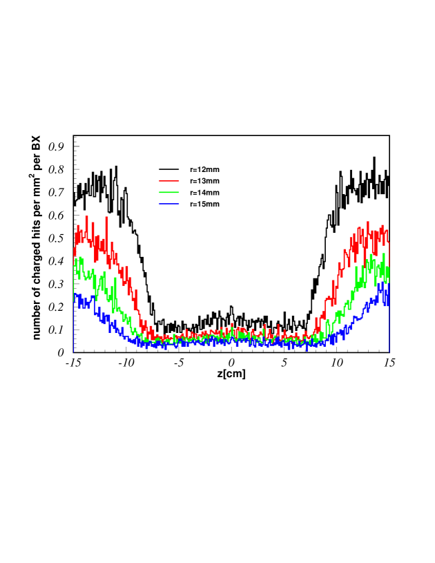
Figure 1: The background hit densities at TESLA in each vertex layer as a function of a distance along the beamlines for 3 T magnetic field. From Ref. [11].

In contrast, simulations done for the NLC/JLC VXD [12] result in 3 hits/mm²/train for a 3 T central magnetic field (or 0.03 hits/mm²/bunch). Figure 2 shows the results of these simulations, where number of background hits per bunch is plotted as a function of the magnetic field at various radii. (The 280 hits in Layer 1 for the magnetic field of 3 T, shown in Figure 2, correspond to a hit density of  3 hits/mm²/train.)

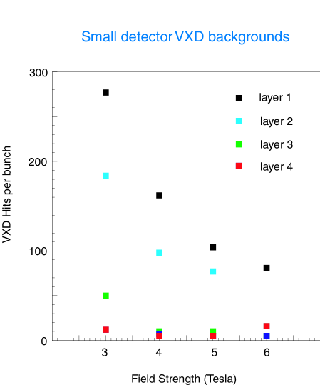
Figure 2: The raw number of hits at NLC in each layer as a function of magnetic field for the small detector. (The masking layout was not modified for the low magnetic field, so hits from pairs which impacted the outer face of the M1 mask were deleted.) From Ref. [12].

Both groups are working on designs of vertex detectors with a first active layer placed at a radial distance of 1.2 cm away from the colliding beams. For both bunch time structures, it is felt that it is possible to operate such detectors with hit densities seen in the simulations.

In addition to beam-induced background sources discussed in the previous studies, overlapping hadronic $\gamma\gamma$ interactions provide a source of background. Preliminary studies of their effect on reconstruction of physics processes of interest, e.g., for Higgs decays, have been done in the ECFA-DESY Study [13]. The authors concluded that a combination of kinematic and vertex topology selections can reduce the effects of $\gamma\gamma$ interactions, with moderate losses in reconstruction efficiency. The background events resulted in a very small additional number of charged hits in the inner layer of the vertex detector in the amount of $3.4\times 10^{-5}$ hits/mm²/bunch.

Optimization work on the mask designs is still in progress, to reduce the beam backgrounds even further. In addition, there are other ideas leading to background reduction, which remain to be evaluated. One possibility, currently under study, is to increase the strength of the magnetic field in the detector. Another option, relevant for the NLC/JLC beam structure, is to reduce the number of bunches recorded by the electronics during the collisions. Such reduction can be achieved by applying pipelined front-end readout with a length of the integration window shorter than the 266 ns duration of the NLC/JLC bunch train. However, the presently achieved reduction factors are very good for both machine designs and result in acceptable levels of background.

3 Higgs Bosons

This section details our study of the physics of the Higgs boson(s). In this report, we consider a Higgs to be any excitation of a field whose vacuum expectation value breaks electroweak symmetry. They arise from the same dynamics as the longitudinal $W^{\pm}$ and $Z^{0}$ bosons. It is an experimental fact that the latter exist, because the $W$ and $Z$ have mass. At the same time, the measured quantum numbers of quarks and leptons unmistakably reveal an $SU(2)_{W}\times U(1)_{Y}$ gauge symmetry mediated by the transverse $W$ and $Z$. These two observations can be reconciled only if the symmetry is spontaneously broken. Then the theory of the Higgs mechanism shows how massless gauge bosons and massless scalars (or Nambu-Goldstone bosons) can interact to form a massive vector boson, and dictates how the physical Higgs bosons couple to $W$ and $Z$.

For example, the standard model contains a complex doublet of fundamental scalar fields. Three of the degrees of freedom in the doublet become the longitudinal modes of the $W^{\pm}$ and $Z^{0}$, while the fourth becomes the single Higgs boson of this model. The standard model’s doublet also generates masses for quarks and charged leptons. The true nature of the Higgs sector remains experimentally obscure, however. It could be richer, with several Higgs bosons sharing in the mass generation of $W$ and $Z$, with some or all of them generating the fermion masses. And the full mechanism that breaks the electroweak symmetry should contain additional particles as well, probably at the TeV scale.

At an LC the process $e^{+}e^{-}\to Z^{*}\to ZH$ gives a superb way to search for Higgs bosons, without relying on the decay products of the $H$. If several fields give mass to the $Z$, several Higgs states may be found in this way. Even if the dominant branching ratio is to invisible particles, a Higgs still could be observed easily as a bump in the missing mass recoiling against the $Z$, perhaps even when broad. Under these and other circumstances, the LC also could observe Higgs bosons that would escape detection at hadron colliders.

As explained in the introduction, we will focus on a Higgs boson with couplings similar to the one in the standard model. We do not necessarily believe that this is the most likely situation, or the most interesting. But it is a well-motivated example, because most manifestly viable models have a limit, called the decoupling limit, for which sub-TeV phenomena can be described by the standard model, plus small corrections from higher-mass states, which would be produced only at the LHC or a multi-TeV LC.

Figure 3 shows the branching ratios for decays of the standard model Higgs boson $H$, as a function of its mass [15].

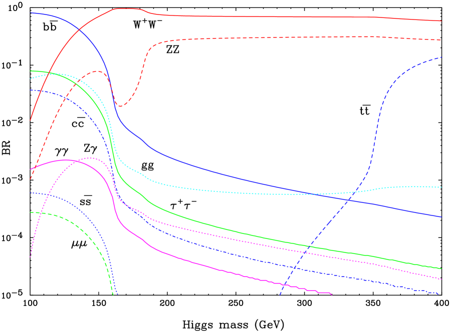
Figure 3: Branching ratios for the Higgs boson in the standard model, as a function of Higgs mass $m_{H}$, as computed by HDECAY [15].

There are four qualitatively different regions:

1. very light Higgs, $m_{H}\mathop{\raisebox{-1.72218pt}{\hbox to0.0pt{$\sim$\hss}}\raisebox{1.72218pt}{$<$}}113$ GeV. The largest standard branching ratios are $b\bar{b}$, $\tau^{+}\tau^{-}$, $c\bar{c}$, $gg$, and $\gamma\gamma$. The last two proceed through loop processes. At the highest masses in this range $W^{\pm}W^{\mp*}$ and $ZZ^{*}$ branching ratios should be observable.

2. light Higgs, $113~{}{\rm GeV}\mathop{\raisebox{-1.72218pt}{\hbox to0.0pt{$\sim$\hss}}\raisebox{1.72218pt}{$<$}}m_{H}<2m_{W}$. The branching ratios to $b\bar{b}$, $c\bar{c}$, $\tau^{+}\tau^{-}$, $W^{\pm}W^{\mp*}$, $ZZ^{*}$ are all measurable, as are the loop-mediated decays $gg$, $\gamma\gamma$, and $Z\gamma$.

3. intermediate Higgs, $2m_{W}<m_{H}<2m_{t}$. The branching ratios to $WW$ and $ZZ^{(*)}$ are large and easy to measure. The decay to $b\bar{b}$ is rare; to $gg$, $c\bar{c}$ and $\tau^{+}\tau^{-}$ very rare.

4. heavy Higgs, $m_{H}>2m_{t}$. Similar to case 3, but now the branching ratio to $t\bar{t}$ should be measurable.

In cases 1 and 2, the total width of the Higgs is narrow and must be determined indirectly. As we explain below, the LC can do so in a model-independent way. It is broad enough in cases 3 and 4 to allow a direct measurement at either the LHC or an LC.

The appeal of the LC is extremely strong in cases 1 and 2. Case 1 is ruled out by non-observation at LEP, unless the Higgs has a non-standard coupling to $Z$ or decays in a non-standard way. Some regions of the parameter space in supersymmetric models allow such behavior, and it is a feature of several other models too. These scenarios also can pose problems for the LHC, either in observation or elucidation. In case 2 the standard-model-like Higgs is a bonanza for an LC, already at modest $\sqrt{s}$. With the expected luminosity, several tens of thousands of Higgs bosons should be produced. The LC would be in a position to check experimentally a remarkable feature of the standard model, namely that the same Higgs field gives mass to gauge bosons, charged leptons, up-type quarks, and down-type quarks. In fact, the precision should be enough to probe the effects of virtual corrections from higher-mass particles.

On the other hand, if the decay to real $W^{+}W^{-}$ pairs is kinematically allowed (cases 3 and 4), it and the similar decay to $ZZ^{*}$ or real $ZZ$ swamp the rates to quarks and charged leptons. The integrated luminosity needed to measure the $b\bar{b}$ branching ratio, not to mention the $c\bar{c}$ and $\tau^{+}\tau^{-}$, has not been thoroughly investigated. We make a first attempt below, showing that ingenuity as well as very high integrated luminosity will be needed, but we have not even started to worry about systematic limitations.

With this background in mind, the rest of this section covers what hadron colliders at Fermilab and CERN can do (very briefly) and then reviews the main measurements that an LC can add. The latter is based mostly on published work and focuses on the light Higgs. We add to this a discussion on how to measure the spin and parity of a light Higgs boson. Next, we revisit the arguments for a light Higgs. We note that the data-driven upper bound, currently at 170 GeV at 95% confidence level, assumes that the standard model is valid up to very high scales. This assumption is not likely to be right, and if the standard model is treated as an effective theory, the bounds are much weaker. Thus, we also consider properties of a standard-model(-like) Higgs boson of intermediate or heavy mass.

3.1 Higgs Physics at Hadron Colliders

3.1.1 Discovery potential

Now that LEP has ended running, it will be the task of Run II of the Fermilab Tevatron or of the CERN Large Hadron Collider (LHC) to determine if a Higgs sector does indeed exist, or some other mechanism is responsible for electroweak symmetry breaking and fermion mass generation. Higgs physics in hadronic collisions is complicated by the presence of several production mechanisms, and the presence of hadronic backgrounds that obscure some final states. Nevertheless, it is clear that the LHC especially will provide a wealth of information on the Higgs boson, and the contribution of the LC must be weighed against it.

The Tevatron’s $p\bar{p}$ collision energy has been raised to $\sqrt{s}=2$ TeV, increasing several theoretical Higgs production cross sections considerably. The coinciding luminosity upgrade grants it significant potential to discover a (standard-model-like) Higgs boson, up to about 180 GeV via a combinatorial analysis of several channels [14]. The search strategy requires large integrated luminosity, 15 fb^-1 or more. In certain scenarios in the minimal supersymmetric standard model (MSSM), Tevatron’s discovery potential is dramatically better than in the standard model. There are, however, also large regions of parameter space in which the Higgs boson would be unobservable. Furthermore, even if a Higgs-like state is observed at the Tevatron, it will be a challenge to measure accurately enough its properties so as to distinguish the underlying model. Largely this is a function of luminosity: with even twice as much data as anticipated, one may be able to draw some conclusions about the nature of the Higgs sector, such as couplings and spin.

If no Higgs boson is observed at the Tevatron, then attention will shift to the LHC. Its $pp$ collisions at $\sqrt{s}=14$ TeV will have enough energy to produce a Higgs of any mass, up to the unitarity constraint of about 1 TeV. The LHC is also a good machine for determining the structure of a Higgs sector. We outline here both the likely discovery modes of a standard-model Higgs at the LHC, as a function of the Higgs mass, and measurement prospects for the quantum numbers which would define the Higgs sector observed.

The dominant production mode over the entire possible mass range of the Higgs is gluon-gluon fusion, $gg\to H$. At all Higgs masses above the experimental limit, weak boson fusion (WBF) is the next largest cross section, about a factor of 8 smaller than gluon fusion over most of the mass range. The associated production modes—$WH$, $ZH$, $t\bar{t}H$—have cross sections that fall off swiftly as the Higgs mass increases. In each case one must consider several different decay channels, depending on the mass, as discussed above. Neither the size of the production cross section nor the dominant branching ratio is a good indicator of the best discovery channel. Discovery potential is instead a complicated function of the relative size of the cross sections, the decay mode under consideration, and the richness of the final event structure. The last is important for providing discriminating power against the enormous QCD backgrounds that will be present at the LHC. For instance, if $m_{H}=120$ GeV, the dominant branching ratio is to $b$ quark pairs, but the QCD background to $gg\to H\to b\bar{b}$ is about five orders of magnitude larger, making observation of this channel hopeless. It is more promising to examine WBF events, which naturally yield far-forward and far-backward jets of very high energy for tagging, or associated $t\bar{t}H$ production, in which complicated event structures are found. Another alternative is to use other final states: although they have smaller branching ratios, the backgrounds are often much less severe.

With this overview in mind, the following paragraphs sketch the likely standard-model Higgs discovery channels, as a function of Higgs mass.

$\bullet$ Higgs mass from 110 to 125 GeV

For this mass range, the significant decays are to $b\bar{b}$ and $\tau^{+}\tau^{-}$. The rare decay $H\to\gamma\gamma$ is important, however, owing to drastically lower backgrounds. At present, $t\bar{t}H$ associated production is the only channel in which an observation of $H\to b\bar{b}$ has been shown to be feasible. CMS and ATLAS studies indicate that this would require 100 fb^-1 or more of integrated luminosity to reach $5\sigma$ [16, 17]. With 30–50 fb^-1 both ATLAS and CMS can reach $5\sigma$ in several other channels: $gg\to\gamma\gamma$, $qq^{\prime}\to qq^{\prime}\gamma\gamma$, $qq^{\prime}\to qq^{\prime}\tau^{+}\tau^{-}$ [16, 17], and, for $m_{H}>115$ GeV, $qq^{\prime}\to qq^{\prime}WW$ [18]. For photon pairs in gluon fusion, the backgrounds are extremely large and CMS can probably perform better than ATLAS due to its better photon mass resolution. Thus, for CMS, discovery in this mass range is likely to be via gluon fusion Higgs production and decay to a pair of photons. For ATLAS, the situation is somewhat less certain. With 50 fb^-1, it would be able to observe all four modes mentioned above at approximately the same significance, somewhat above $5\sigma$, but pending full detector simulation one cannot confidently guess which one will win out. But this is rather moot, as both experiments would enjoy the confidence of confirming discovery in multiple channels, nearly simultaneously.

$\bullet$ Higgs mass from 125 to 200 GeV

For $m_{H}\mathop{\raisebox{-1.72218pt}{\hbox to0.0pt{$\sim$\hss}}\raisebox{1.72218pt}{$>$}}125$ GeV, the decay $H\to W^{(*)}W^{(*)}$ becomes very significant. Due to the uniqueness of the signature $W^{(*)}W^{(*)}\to e\mu/\!\!\!p_{T}$, in both gluon fusion and WBF production modes, discovery potential shifts from the fermionic or rare decays to these channels. Although gluon fusion has a much higher signal rate than WBF, it is not as clean as WBF, and the channels turn out to be competitive with each other.

For $m_{H}<150$ GeV or so, the WBF channel is probably somewhat better, although this has not yet been explored fully by the detector collaborations. In particular, $gg\to H\to W^{(*)}W^{(*)}$ has not been explored in published form by the collaborations for $m_{H}<150$ GeV. The WBF channel would require approximately 10–15 fb^-1 at $m_{H}=125$ GeV [18], but the amount of data required for a $5\sigma$ observation drops rapidly with increasing Higgs mass, to only 5 fb^-1 at $m_{H}=140$ GeV [19]. For $m_{H}\mathop{\raisebox{-1.72218pt}{\hbox to0.0pt{$\sim$\hss}}\raisebox{1.72218pt}{$>$}}150$ GeV, both gluon fusion and WBF would require less than 5 fb^-1, or half a year of running at design turn-on luminosity of the LHC. We note that the studies of $gg\to H\to W^{(*)}W^{(*)}$ have not yet taken advantage of the transverse mass distribution of the $W$ pair, as the WBF studies have, so prospects there may improve somewhat [20]. Considering the short amount of time after turn-on that a discovery could be made, however, a discovery would probably be announced in both channels simultaneously, again providing additional confidence.

$\bullet$ Higgs mass above 200 GeV

Above $m_{H}=200$ GeV the only decay channels to consider for discovery potential are those to weak bosons, $H\to W^{+}W^{-},ZZ$ [16, 17]. Above $m_{H}=350$ GeV, the decays $H\to t\bar{t}$ require large integrated luminosity and, thus, cannot compete. The channel $gg\to H\to ZZ\to 4\ell$ is clearly extremely powerful, requiring less than 5 fb^-1 of integrated luminosity up to about 400 GeV in Higgs mass, and about 5 fb^-1 up to 500 GeV. Above $m_{H}=400$ GeV, it is likely that production by gluon fusion would provide the quickest discovery, simply due to the higher rate and low backgrounds: $S/B\gg 1/1$ for gluon fusion in this mass range.

3.1.2 Width measurements

Beyond discovery of a Higgs-like resonance, experiments must measure its couplings to standard particles and test whether it behaves like the one-doublet or some other Higgs sector. One may trade these couplings for Higgs partial decay widths, the sum of which is the Higgs total width. The Higgs total width grows with $m_{H}$, and does not exceed experimental resolution in direct reconstruction for Higgs masses below about 220 GeV. For this range, width resolution is several tens of percent, falling off to $\sim 10\%$ around $m_{H}=300$ GeV, and achieving a best value of $\sim 3$–$4\%$ for $m_{H}=400$ GeV [16, 17].

For $120<m_{H}<200$ GeV, the total width can be determined indirectly for a standard Higgs sector by summing up the observed decay branching ratios in several different channels. Phenomenological studies suggest the decay width to $W^{+}W^{-}$ in such a scenario could be measured to about 8–$10\%$, depending on the Higgs mass. The width to $ZZ$ cannot be measured quite as well, but one can improve its resolution by assuming the $SU(2)$ relation between $\Gamma_{H\to WW}$ and $\Gamma_{H\to ZZ}$. For Higgs masses where decays to tau pairs are visible, the partial width to $\tau^{+}\tau^{-}$ could also be measured: $\Gamma_{H\to\tau\tau}/\Gamma_{H\to WW}$ could be determined to about 10–$20\%$ [21]. Then, because the width to $b\bar{b}$ is not measured at LHC, one must calculate $\Gamma_{H\to b\bar{b}}$ from the measured $\Gamma_{H\to\tau\tau}$. In this way one can determine the total width of the Higgs to 10–20%, with better accuracy for larger Higgs mass [21]. Nevertheless, one should keep in mind the theoretical assumptions that are required to extract the width from the measurements. In particular, in the light region, where $H\to b\bar{b}$ dominates, one must assume that the same Higgs boson generates $m_{b}$ and $m_{\tau}$.

For a Higgs sector that is not very much like the standard model, these indirect measurements can become much more complicated. In general one would be able to detect deviations from the standard model by taking ratios of partial widths, but the uncertainties in width extractions are complicated functions of the model. Recent work suggests that the LHC will have good capability to detect invisible Higgs branching ratios as small as $15\%$, but this would require a modification to the current ATLAS and CMS trigger designs [22].

3.1.3 Spin determination and $CP$ properties

Any narrow resonance observed at the LHC with Higgs-like couplings would have to be confirmed to be spin zero. The LHC can do a fairly good job at this, but has difficulty for Higgs masses above 400 GeV. First, if $H\to\gamma\gamma$ is observed, the Landau-Yang Theorem implies that the resonance is not a vector, cf. Sec. 3.3. The more powerful technique, however, which works for $130\mathop{\raisebox{-1.72218pt}{\hbox to0.0pt{$\sim$\hss}}\raisebox{1.72218pt}{$<$}}m_{H}\mathop{\raisebox{-1.72218pt}{\hbox to0.0pt{$\sim$\hss}}\raisebox{1.72218pt}{$<$}}400$ GeV, is to examine the azimuthal distribution of the reconstructed pairs of $Z$ bosons in $gg\to H\to ZZ\to\ell^{+}\ell^{-}\ell^{+}\ell^{-}$ [16, 17]. This measurement does require large statistics, but has good discriminating power. Recent work [23], examining the azimuthal distribution of the tagging jets in $qq^{\prime}\to Hqq^{\prime}$, demonstrates that the LHC can determine the $CP$ nature of a light Higgs, as well as the tensor structure of the $HWW$ vertex. An LC can carry out such studies with higher precision, however.

3.1.4 Higgs self-coupling

Exploration of a Higgs sector would not be complete without also measuring the Higgs self-coupling $\lambda$. In the standard model this is the free parameter that fixes the Higgs mass. In models with two Higgs doublets there is more than one self-coupling; for the MSSM these become gauge couplings and are rigidly determined. $\lambda$ can be determined only via direct production of two or more Higgs bosons, the standard-model cross section for which is extremely small at the LHC and the backgrounds are large. Thus, it is probable that the LHC cannot make a measurement here [24].

3.2 Light Higgs at LC

If the Higgs boson has a mass between LEP’s lower limit and $2m_{W}$, the LC can verify experimentally the main features of the Higgs mechanism. It can also measure small deviations from the standard model, which indicate higher-mass states coupled to the Higgs. This is a very exciting prospect. This subsection reviews how the coupling of the Higgs to other particles and to itself will be attained. A full description of the light Higgs physics program is outlined in Refs. [25, 2, 3].

The two main production channels are $e^{+}e^{-}\to Z^{*}\to ZH$ and $e^{+}e^{-}\to\bar{\nu}_{e}W^{+*}W^{-*}\nu_{e}\to\bar{\nu}_{e}H\nu_{e}$. With standard-model couplings to $Z$ and $W$, the LC will produce several tens of thousands of Higgs bosons this way, given design luminosity of around 300 ${\rm fb}^{-1}{\rm yr}^{-1}$. The results [26] for branching ratios of a recent simulation of Higgs production in $500~{}{\rm fb}^{-1}$ at $\sqrt{s}=350$ GeV is shown in Fig. 4(a).

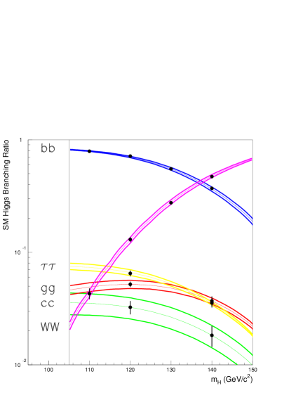
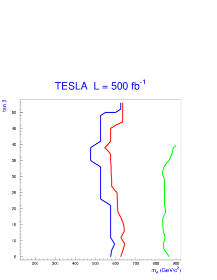
Figure 4: Simulation of a standard-model Higgs, assuming $\int{\cal L}dt=500~{}{\rm fb}^{-1}$ and $\sqrt{s}=350$ GeV. From Ref. [26]. (a) Simulated uncertainties in branching ratios vs. $m_{H}$. (b) Reach in the mass $m_{A}$ of the $CP$-odd state of the MSSM; from left to right the curves exclude 95%, 90%, and 68% of the parameter space considered in Ref. [26].

This study relies on developments in heavy flavor tagging to separate $b$- and $c$-flavored jets from each other and from jets with light hadrons. As one can see, these measurements would be good enough to show that the putative Higgs boson generates mass for vector bosons, charged leptons, down-type quarks, and up-type quarks. Through $H\to{\rm loop}\to gg$, it would also probe for non-standard colored particles coupling to $H$.

These measurements would yield a wealth of information. They test the one-doublet model, in which the ratio of branching ratios of particles coupling directly to the Higgs should correspond to the ratio of squared masses. They also test indirectly for more massive states, which produce radiative corrections or mixing effects that modify the ratio test. These deviations diminish for higher mass, so the higher the integrated luminosity, the higher the reach. This is illustrated in Fig. 4(b), which gives bounds on the mass $m_{A}$ of the $CP$-odd Higgs of the MSSM. Because this analysis [26] studies only part of the MSSM parameter space, the numerical reach given here is not definitive. A more recent study [27] finds a similar reach, except in small regions of MSSM parameter space where the $h^{0}$ has exceptionally standard properties. Nevertheless, this kind of analysis indicates that a compelling program of precision physics is possible.

The LC also gives an indirect, but model-independent, measurement of the total width. (A light Higgs is narrower than the mass resolution.) The production cross section for $ZH$ ($H\bar{\nu}\nu$) depends on the partial width $\Gamma_{H\to ZZ}$ ($\Gamma_{H\to WW}$). Thus, independent measurements of the cross section and the branching ratio can be combined to obtain the full width without theoretical assumptions. A recent study finds an uncertainty on the width of 5–10% when $m_{H}<2m_{W}$ [28], somewhat better than at the LHC. The essential contribution of the LC would be to determine the width with no theoretical ingredients.

The LC can also study $t\bar{t}H$ events to measure the top Yukawa coupling [29]. As with the branching ratio tests, the result can be compared with the top mass, to check how much of $m_{t}$ the $H$ at hand generates. At $\sqrt{s}=500$ GeV there are not many events. At $\sqrt{s}=800$ GeV a simulation has been carried out recently for $m_{H}=120$ GeV, with realistic treatment of backgrounds and detector performance [30]. Assuming $1000~{}{\rm fb}^{-1}$ of integrated luminosity the study finds a systematic (statistical) uncertainty of 5.5% (4.2%).

Finally, the self-coupling $\lambda$ can be measured from the rate of $ZHH$ events [31]. The cross section is small, so luminosity is especially valuable here. A study assuming $\int{\cal L}dt=500~{}{\rm fb}^{-1}$ and $\sqrt{s}=500$ GeV has been started. A measurement at the ten percent level seems feasible, once the procedure has been optimized [32].

3.3 $J^{PC}$ of the Higgs Particle

In this section we examine how to determine the $J^{PC}$ quantum numbers of a (putative) Higgs boson. The Higgs boson of the Standard Model has, by construction, $J^{PC}=0^{++}$. The strengths and space-time structure of its couplings to vector bosons are uniquely determined, as they come from the covariant derivative $(D_{\mu}\phi)(D^{\mu}\phi)$ terms in the Lagrangian. Models with more Higgs doublets have additional neutral particles. For example, with two doublets there are three neutral particles, $h^{0}$, $H^{0}$, and $A^{0}$. Neglecting $CP$ violation, the first two are $CP$-even and the last is $CP$-odd. In general the mass eigenstates will be $CP$ mixtures, and with $CP$ violation in the Higgs sector the mixing could be significant.

Once one or more new states have been observed at the Tevatron, LHC and/or LC, a determination of their quantum numbers and the nature of their couplings to vector bosons will be a crucial step toward understanding electroweak symmetry breaking. It is hard to unravel $CP$ mixtures, so we defer discussion of the difficulties and some prospects based on interference measurements to Sec. 3.3.5. There are several straightforward ways to obtain information on the spin: decay to $\gamma\gamma$ implies that the parent state cannot have spin one (Sec. 3.3.1); the rise of the $ZH$ threshold depends on the spin of the $H$ (Sec. 3.3.2); and angular distributions of $ZH$ production and decay are diagnostic of spin (Sec. 3.3.4). The first is accessible to the LHC, the second and third are possible only with a lepton collider. This section focuses on Higgs bosons, but these experimental characteristics can be extended to other bosons as well.

3.3.1 Decays of a putative $H$ boson to $\gamma\gamma$

Observation of the decay $H\to\gamma\gamma$ places restrictions on the possible spin of a putative Higgs boson. For the light Higgs, the decay $H\to\gamma\gamma$ is a discovery mode at the LHC. Then, the Landau-Yang theorem [33] ensures that $H$ cannot have spin one. Sakurai [34] gives a proof of this in the context of $\pi^{0}\to\gamma\gamma$, and given the importance of this argument, we remind the reader of Sakurai’s version of its proof.

Let us assume $H\to VV$ decay, where $VV$ are identical massless vector bosons. In momentum space the final state wave function can be constructed from the polarization vectors $\mbox{\boldmath$\epsilon$}_{1}$ and $\mbox{\boldmath$\epsilon$}_{2}$ and the relative momentum three-vector $k$. This wave function must be linear in $\mbox{\boldmath$\epsilon$}_{1}$ and $\mbox{\boldmath$\epsilon$}_{2}$, and if the $H$ has spin one it must transform like a vector under rotations. By Bose symmetry, the wave function must be symmetric under the interchange $\mbox{\boldmath$\epsilon$}_{1}\leftrightarrow\mbox{\boldmath$\epsilon$}_{2}$ and $\mbox{\boldmath$k$}\leftrightarrow-\mbox{\boldmath$k$}$. The possible combinations $\mbox{\boldmath$\epsilon$}_{1}\times\mbox{\boldmath$\epsilon$}_{2}$ and $(\mbox{\boldmath$\epsilon$}_{1}\cdot\mbox{\boldmath$\epsilon$}_{2})\,\mbox{\boldmath$k$}$ for the $H$ transformation rule are ruled out because they are antisymmetric under the interchange. The combination $\mbox{\boldmath$k$}\times(\mbox{\boldmath$\epsilon$}_{1}\times\mbox{\boldmath$\epsilon$}_{2})$ is symmetric, but $\mbox{\boldmath$k$}\times(\mbox{\boldmath$\epsilon$}_{1}\times\mbox{\boldmath$\epsilon$}_{2})=\mbox{\boldmath$\epsilon$}_{1}\,(\mbox{\boldmath$k$}\cdot\mbox{\boldmath$\epsilon$}_{2})-\mbox{\boldmath$\epsilon$}_{2}\,(\mbox{\boldmath$k$}\cdot\mbox{\boldmath$\epsilon$}_{1})=0$, because $\mbox{\boldmath$k$}\cdot\mbox{\boldmath$\epsilon$}_{i}=0$ for massless vector bosons. Thus if the decay $H\to\gamma\gamma$ is observed, one can immediately rule out the possibility that $H$ is spin one.

A similar conclusion holds when $V$ is a stable, massive vector boson, but not for the $Z$ boson. The $Z$’s non-zero width means that it is essentially always off shell.

3.3.2 Production process

A useful reaction for studies of the Higgs quantum numbers is $e^{+}e^{-}\to ZH$ with the subsequent leptonic decay of the $Z$. The cross section is

$$\sigma(ZH)=\frac{G_{F}^{2}m_{Z}^{4}}{96\pi s}\left(a_{e}^{2}+v_{e}^{2}\right)\beta\frac{\beta^{2}+12m_{Z}^{2}/s}{\left(1-m_{Z}^{2}/s\right)^{2}}$$ (1)

where $a_{e}$ is the axial and $v_{e}$ the vector coupling of the electron. (In the standard model, $a_{e}=-1$ and $v_{e}=-1+4\sin^{2}\theta_{W}$.) The factor

$$\beta^{2}=\frac{4|\mbox{\boldmath$p$}_{Z}|^{2}}{s}=\left(1-\frac{(m_{H}+m_{Z})^{2}}{s}\right)\left(1-\frac{(m_{H}-m_{Z})^{2}}{s}\right)$$ (2)

arises from two-particle phase space. The single power of $\beta$ is characteristic of scalar-vector production, so the threshold behavior is already diagnostic (see Sec. 3.3.3).

Events of the associated $ZH$ production can be selected independent of the Higgs decay modes, by requiring the missing mass relative to the $Z$ boson to be near the known Higgs mass. The background will come from processes with $Z$ bosons in the final state, principally $e^{+}e^{-}\to ZZ$, $e^{+}e^{-}\to Z\gamma^{*}$, and $e^{+}e^{-}\to\gamma^{*}\gamma^{*}$. In the case of $m_{H}=120$ GeV and $\sqrt{s}=500$ GeV, the expected numbers of events for 500 ${\rm fb}^{-1}$ are shown in Table 2.

Table 2: Cross sections and event rates for 500 ${\rm fb}^{-1}$.

Process	$\sigma$ (fb)	# of events	# of $Z\to e,\mu$
$ZH$	66	33000	2040
$ZZ$	660	330000	44000
$Z\gamma^{*}+\gamma^{*}\gamma^{*}$	9500	475000	158000000

It is expected that a clean sample of $ZH$ events can be identified despite the potentially large background. This is especially true for a light Higgs boson with a significant branching fraction for $H\rightarrow b\bar{b}$ decays. In this case a relatively modest vertex detector will reduce the background in the $ZH$ events sample to a level below a few percent.

3.3.3 Constraining $J^{PC}$ from the cross section at threshold

As mentioned in Sec. 3.3.2, the behavior of the $ZH$ production cross section at threshold allows one to constrain the possible values of $J^{PC}$ of the putative Higgs boson. In Ref. [35] it is shown that the dependence of the cross section at threshold on $\beta$ distinguishes between different spin-parity properties of a putative Higgs boson produced in Higgsstrahlung. In particular, if the cross section grows like $\beta$ at threshold then $H$ must be a $CP$-even scalar, a $CP$-even vector (i.e. a pseudo-vector), or a $CP$-even spin-2 object. For all other spin-parity assignments, including the $CP$-odd scalar, $CP$-odd vector, $CP$-odd spin-2 object, and spins higher than two with either parity, the cross section at threshold grows like $\beta^{3}$ or higher powers.

To distinguish between the three spin-parities that give a linear rise with $\beta$ in the Higgsstrahlung cross section at threshold, other techniques must be used. The observation of the decay $H\to\gamma\gamma$, discussed above in Sec. 3.3.1, immediately rules out spin one. Angular distributions, discussed below in Sec. 3.3.4, allow one to distinguish between the possible spin-parity assignments. Finally, with enough integrated luminosity doubly-differential angular distributions can remove any ambiguities remaining for the threshold behavior and singly-differential angular distributions.

3.3.4 Determination of $J^{PC}$ from angular distributions

The reaction $e^{+}e^{-}\to ZX$ provides a very clean test for the quantum numbers of the particle $X$. In a general model, a scalar can couple to $VV$ through a dimension-3 operator $\phi_{S}V^{\mu}V_{\mu}$. A pseudoscalar can couple to $VV$ through a dimension-5 operator, $\phi_{P}F^{\mu\nu}\tilde{F}_{\mu\nu}$. The pseudoscalar coupling to vector pairs can be large, for example in topcolor models where $\phi_{P}$ denotes the topcolor pion. Several observables are sensitive to the spin-parity of the $X$:

• the angular distribution of the $X$ decay products in its center-of-mass system, which depends, in general, on the $X$ decay mode, and so differs for $X\to f\bar{f}$ and $X\to VV$.

• the distribution in $\cos\theta$, where $\theta$ is the angle between the $e^{-}$ and the $Z$.

• the distribution in $\cos\theta^{*}$, where $\theta^{*}$ is the angle between the final-state $e^{-}$ or $\mu^{-}$ and the $Z$ direction of motion, in the $Z$ center-of-mass system.

• the distribution in $\varphi^{*}$, where $\varphi^{*}$ is the angle between the $Z$ production plane and the $Z$ decay plane.

In the case of $J^{PC}=0^{++}$ (i.e., $X=h,\,H$) the differential cross section is [36]

$$\begin{split}\frac{d^{3}\sigma(ZH)}{d\cos\theta d\cos\theta^{*}d\varphi^{*}}\sim&\,\sin^{2}\theta\sin^{2}\theta^{*}-\frac{1}{2\gamma}\sin 2\theta\sin 2\theta^{*}\cos\varphi^{*}\\ +&\;\frac{1}{2\gamma^{2}}\left[(1+\cos^{2}\theta)(1+\cos^{2}\theta^{*})+\sin^{2}\theta\sin^{2}\theta^{*}\cos 2\varphi^{*}\right]\\ -&\;\frac{2v_{e}a_{e}}{v_{e}^{2}+a_{e}^{2}}\frac{2v_{f}a_{f}}{v_{f}^{2}+a_{f}^{2}}\frac{2}{\gamma}\left[\sin\theta\sin\theta^{*}\cos\varphi^{*}-\frac{1}{\gamma}\cos\theta\cos\theta^{*}\right],\end{split}$$ (3)

where $\gamma$ is the Lorentz boost of the $Z$ boson. In the $0^{-+}$ case (i.e., $X=A$) the corresponding cross section is

$$\begin{split}\frac{d^{3}\sigma(ZA)}{d\cos\theta d\cos\theta^{*}d\varphi^{*}}\sim&\,1+\cos^{2}\theta\cos^{2}\theta^{*}-\frac{1}{2}\sin^{2}\theta\sin^{2}\theta^{*}\\ -&\;\frac{1}{2}\sin^{2}\theta\sin^{2}\theta^{*}\cos 2\varphi^{*}+2\frac{2v_{e}a_{e}}{v_{e}^{2}+a_{e}^{2}}\frac{2v_{f}a_{f}}{v_{f}^{2}+a_{f}^{2}}\cos\theta\cos\theta^{*}.\end{split}$$ (4)

The distinctive difference in these angular distributions provides a basis for distinguishing between the two cases.

The triply-differential angular distributions of Eqs. (3) and (4) contain non-trivial correlations between the production angle $\theta$ and the decay angles $\theta^{*}$ and $\varphi^{*}$. Most of these correlations do not contribute to doubly- or singly-differential distributions. A fit to doubly-differential distribution $d^{2}\sigma(ZA)/d\cos\theta d\cos\theta^{*}$ of the corresponding event samples yields a 14$\sigma$ separation between the $0^{++}$ and the $0^{-+}$ cases, see Fig. 5.

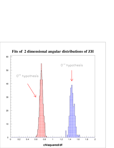
Figure 5: Fits of two-dimensional angular distributions of samples of $ZH$ events with the scalar and pseudoscalar hypothesis.

A powerful test of the spin-parity of the Higgs boson consists of determination of the contribution of separate terms of the angular distributions, Eq. (3). Besides a strong confirmation of the expected $J^{PC}$ assignment, such decomposition can provide limits on a non-standard $ZZH$ coupling, even for the $0^{++}$ case. The statistical power of such an analysis of a sample of events corresponding to a large integrated luminosity of 1250 fb^-1 is shown in Table 3 and illustrated in Fig. 6.

Table 3: Comparison of expected and measured contributions to the 3-D angular distribution.

Term	Expected, Eq. (3)		Measured
$\sin 2\theta\sin 2\theta^{*}\cos\varphi^{*}$	$-0$.	185	$-0$.189$\pm$	0.037
$(1+\cos^{2}\theta)(1+\cos^{2}\theta^{*})$	0.	0682	0.082$\pm$	0.010
$\sin\theta\sin\theta^{*}\cos\varphi^{*}$	0.	0682	0.080$\pm$	0.014
$\sin^{2}\theta\sin^{2}\theta^{*}\cos 2\varphi^{*}$	0.	015	0.030$\pm$	0.074
$\cos\theta\cos\theta^{*}$	0.	006	0.010$\pm$	0.071

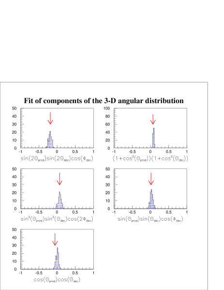
Figure 6: Fits of separate terms of the three-dimensional angular distributions, Eq. (3), of samples of $ZH$ events. The relative weights of the separate terms, with respect to $\sin^{2}(\theta)\sin^{2}(\theta^{*})$ expected from Eq. (3) are indicated by the arrows.

3.3.5 Measuring $CP$ properties of a scalar boson

As described in the previous section, to distinguish models with large scalar or pseudoscalar couplings to vector boson pairs, it is useful to determine which operator the coupling comes from, by measuring angular distributions in $e^{+}e^{-}\to ZX$. These and other methods can also be used to determine the $CP$ properties of a mixed-$CP$ state. One would first like to distinguish a $CP$-even Higgs boson from a $CP$-odd Higgs boson, and, second, to be able to determine whether the observed Higgs boson is a $CP$ mixture and, if so, measure the odd and even components.

The angular dependence of the $e^{+}e^{-}\to ZH$ cross section depends upon whether the Higgs boson $H$ is $CP$-even, $CP$-odd, or a mixture [35, 36, 37, 38]. Following Ref. [38] we parametrize the $ZZH$ vertex as

$$\Gamma_{\mu\nu}(k_{1},k_{2})=ag_{\mu\nu}+b\frac{k_{1\mu}k_{2\nu}-g_{\mu\nu}k_{1}\cdot k_{2}}{m_{Z}^{2}}+\tilde{b}\frac{\varepsilon_{\mu\nu\alpha\beta}k_{1}^{\alpha}k_{2}^{\beta}}{m_{Z}^{2}}$$ (5)

where $k_{1}$ and $k_{2}$ are the momenta of the two $Z$s. The first term arises from a standard-model-like $ZZH$ coupling, and the last two from effective interactions that could be induced by high-mass virtual particles. The coupling $\tilde{b}$ violates $CP$, but the other two conserve $CP$. With this vertex the Higgsstrahlung cross section becomes

$$\frac{d\sigma}{d\cos\theta_{Z}}\propto 1+\frac{p_{Z}^{2}}{m_{Z}^{2}}\sin^{2}\theta_{Z}-4\,{\rm Im}\left[\tilde{b}\over\tilde{a}\right]\frac{v_{e}a_{e}}{v_{e}^{2}+a_{e}^{2}}\frac{p_{z}\sqrt{s}}{m_{Z}^{2}}\cos\theta_{Z}+\left|\tilde{b}\over\tilde{a}\right|^{2}\frac{p^{2}_{z}s}{2m_{Z}^{4}}(1+\cos^{2}\theta_{Z})$$ (6)

where $\tilde{a}=a-bE_{Z}\sqrt{s}/m_{Z}^{2}$; $\theta_{Z}$, $p_{Z}$, and $E_{Z}$ are the scattering angle, momentum, and energy of the final-state $Z$ boson; and $v_{e}$ and $a_{e}$ are the vector and axial-vector couplings at the $e^{+}e^{-}Z$ vertex. The term in Eq. (6) proportional to $\cos\theta_{Z}$ arises from interference between the $CP$-even and $CP$-odd couplings in Eq. (5). If the $CP$-odd coupling $\tilde{b}$ is large enough, it can be extracted from the forward-backward asymmetry. Ref. [38] studied whether the couplings $a$, $b$ and $\tilde{b}$ in Eq. (5) could be extracted, using $e^{+}e^{-}\to f\bar{f}H$ from Higgsstrahlung and $ZZ$ fusion, and found the real and imaginary components of the three couplings could be determined from asymmetries. A more general analysis of the $ZZH$ and $Z\gamma H$ couplings, using the so-called “optimal observable” method, found that the $ZZH$ couplings can be well constrained with or without beam polarization, while the $Z\gamma H$ couplings do require beam polarization [39].

It is important to note that any measurement of $CP$ violating observables in Higgs boson production or decay is a measurement of $CP$ violation in the Higgs boson couplings to the particular initial or final state. It is not, however, a direct measurement of the $CP$ content of the Higgs mass eigenstate(s). This has not often been pointed out in the literature. For example, an MSSM Higgs boson could be a half-and-half mixture of the $CP$-even state $H$ and the $CP$-odd state $A$. If one is not too far into the decoupling regime, then the tree-level $CP$-even coupling of $H$ to $Z$ boson pairs (denoted above by $a$) will be non-negligible, while the loop-induced dimension-5 couplings of $H$ and $A$ to $Z$ pairs ($b$ and $\tilde{b}$, respectively) will be very small. A measurement of the couplings $a$, $b$ and $\tilde{b}$ would indicate correctly that the $CP$ violation in the Higgs couplings to vector boson pairs is very small, because $a\gg\tilde{b}$. This does not, however, indicate that the $CP$ mixing in the Higgs mass eigenstate is small.

With this in mind let us first assume that there is no mixing of the $CP$-odd and $CP$-even Higgs bosons. If there is no $CP$ violation in the Higgs sector itself, i.e. if all the Higgs fields have real vacuum expectation values, then only the $CP$-even Higgs fields couple to $ZZ$ and $W^{+}W^{-}$ at tree level. The dimension-5 couplings of the $CP$-even and $CP$-odd Higgs bosons to vector pairs are induced at loop level, and so are loop suppressed. These loop induced couplings are very small: for example, the loop-induced production process $e^{+}e^{-}\to ZA$ has been studied in the MSSM for a 500 GeV LC, and the cross section was found to be below 0.1 fb [40]. Because the $e^{+}e^{-}\to ZA$ cross section is likely to be very small in a general Higgs sector, it may be impractical to measure angular distributions in $ZA$ production. Likewise, in a general Higgs sector the $CP$-odd Higgs branching ratio to $VV$ is likely to be very small, making it difficult to measure angular distributions in decay; for example, in the MSSM the branching ratios of $A\to VV$ are typically well below $10^{-2}$ [41].

As noted above, a mixed-$CP$ Higgs boson is well-motivated in the MSSM [42]. Mixing of $CP$ eigenstates can be induced at the 1-loop level by soft $CP$-violating trilinear couplings between the Higgs bosons and top and bottom squarks. Unfortunately, it is difficult to study the $CP$ mixing through the Higgs couplings to vector boson pairs because the dimension-5 couplings $b$ and $\tilde{b}$ described above are likely to be very small. The mixed-$CP$ Higgs then couples to $VV$ primarily through its $CP$-even component. Thus, $a\gg b,\tilde{b}$, and the coupling is predominantly that of the standard Higgs, suppressed by a mixing angle (since only the $CP$-even component contributes to $a$), and the effects of the dimension-5 couplings $b$ and $\tilde{b}$ on the angular distributions will be small. The mixing-angle suppression is not diagnostic of $CP$ mixing, because the same suppression can arise in any multi-Higgs-doublet model (such as the MSSM) where the $VV$ couplings of $h^{0}$ and $H^{0}$ are suppressed by $\sin(\beta-\alpha)$ and $\cos(\beta-\alpha)$, respectively.

To probe $CP$ mixing in the Higgs mass eigenstate, $CP$-violating observables in which the $CP$-even and $CP$-odd couplings are both large are desirable. The couplings to photon or fermion pairs of $CP$-even Higgs bosons are comparable to those of $CP$-odd Higgs bosons. Three methods making use of these couplings are described in the literature; they employ $s$-channel Higgs production at a photon or muon collider, and none of them is possible at an $e^{+}e^{-}$ LC. At a photon collider with transversely polarized photon beams, the initial state is pure $CP$-even if the polarizations of the beams are parallel, and pure $CP$-odd if the polarizations of the beams are perpendicular. One can then turn on or off the $CP$-even and odd components of a Higgs resonance by changing the orientation of the polarization of the photons. Combining the observables from linearly polarized photons with those from circularly polarized photons, one can disentangle the $CP$-even and $CP$-odd couplings of a Higgs resonance to photon pairs [43].

At a photon collider one can also take advantage of the interference between a Higgs-mediated process and a process with the same final states mediated by something else. This is familiar from the measurement of $CP$ violation in the $B$ and $K$ meson systems. In Ref. [44] the process $\gamma\gamma\to t\bar{t}$ is studied near the Higgs resonance. In this process a Higgs-mediated component of the amplitude interferes with the continuum amplitude enabling one to determine the $CP$ properties of the Higgs.

Finally, one can use fermion polarization to measure the mixed-$CP$ Higgs Yukawa couplings to fermions. In Ref. [45] a muon collider with polarized beams is proposed, to produce Higgs bosons in the $s$ channel through the mixed-$CP$ muon Yukawa coupling, $\bar{\mu}(a+ib\gamma_{5})\mu$. The $CP$-even and $CP$-odd components of the Higgs coupling to muon pairs can be disentangled using transversely polarized muon beams. Similarly, Ref. [46] studies the process $\mu^{+}\mu^{-}\to H\to f\bar{f}$, where $f\bar{f}$ are third-generation fermions. Helicity observables in $\mu^{+}\mu^{-}$ and $f\bar{f}$ allow one to measure the $CP$-even and $CP$-odd components of the Higgs couplings.

3.4 Expected Mass of the Higgs Boson

As discussed at the beginning of this section, the physics of a standard-model-like Higgs boson depends critically on whether the decay to an on-shell $WW$ pair is kinematically allowed or not. It is therefore crucial to review what is known today about the mass of the Higgs boson from indirect measurements and theory. It is impossible to interpret the measurements without some recourse to theory, but we shall do so with as few assumptions about the Higgs sector as possible. In particular, we do not assume that the standard model is a fundamental theory—we know that it is not—but rather an effective field theory, valid up to some scale, denoted here as $\Lambda_{\rm SM}$. This is a very mild assumption, and it weakens well-known bounds based on precise electroweak data, which assume $\Lambda_{\rm SM}\to\infty$.

The most powerful constraints are the precise measurements of the $Z^{0}$ line-shape from SLD and the four LEP experiments, combined with measurements of $\sin^{2}\theta_{W}$ from deeply inelastic scattering, of parity violation in cesium and thallium atoms, of the top quark mass in pair production at the Tevatron, and of the $W$ mass from the Tevatron and LEP experiments. In general, particles beyond each experiment’s kinematic reach contribute to the observables virtually: either in loop processes or as off-shell propagators. For the Higgs boson, and other manifestations of symmetry breaking, the most sensitive contributions are through loops in the $W$, $Z$, and $\gamma$ propagators. These are often called oblique corrections, and it has become customary to summarize them with two parameters, $S$ and $T$, describing the weak isopin-conserving and -violating contributions [47]. (A third quantity $U$, which parametrizes energy-dependent isospin violating effects, can be neglected at $Z$ energies.)

A recent fit to $S$ and $T$ of the precisely measured electroweak observables is shown in Fig. 7(a) [48].

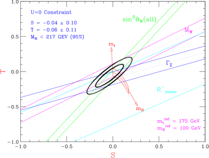
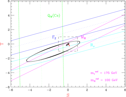
Figure 7: Fits of precisely measured electroweak observables to $S$ and $T$, including 68% confidence bands of the most precise ones [48]. (a) Fit to 14 observables from August 1999. (b) Fit from 1989, with (a) as inset.

Varying $m_{t}$ within the uncertainty of the direct measurement and $m_{H}$ from 100 GeV to 1 TeV traces out the crescent-shaped region. The uncertainty of other standard model parameters, apart from $\alpha_{s}(m_{Z})$, on this region is unimportant. To obtain the crescent the standard model is treated as a fundamental field theory.

The agreement between the crescent for the standard model prediction and the experimentally favored ellipse is not guaranteed. The parameters $S$ and $T$ are defined independently of unknown short-distance physics and are determined from the data with only well-substantiated aspects of the electroweak theory. One may think of the ellipse, therefore, as an experimental measurement. The crescent, on the other hand, is a theoretical prediction of a particular model of the Higgs sector, namely, the standard one with one doublet. The overlap of the two regions demonstrates that the one-doublet model is a very good description of the data.

Other models trace out different regions. For example, the MSSM’s region overlaps with the ellipse in the decoupling limit, when all superpartners are heavy. The MSSM also agrees with the fit when only squarks and sleptons are heavy, but charginos and neutralinos are light—as light as 100 GeV [49]. Early models of technicolor, which do not possess a decoupling limit, trace out regions at significantly larger $S$. Models with composite Higgs bosons trace out regions connected to the standard crescent, but extending to somewhat larger $T$: for them the data allow an intermediate-mass or even heavy Higgs. In this way, the constraints of the data are incisive in deciding what extensions of the standard model should be taken seriously: any model with a decoupling limit naturally agrees with the data just as well as the standard model.

It is common to distill the fit of Fig. 7 into a constraint on $\log(m_{H}/m_{Z})$. This process yields the well-known “blue band” plot of the LEP Electroweak Working Group [50], shown in Fig. 8, and equivalent results from other groups.

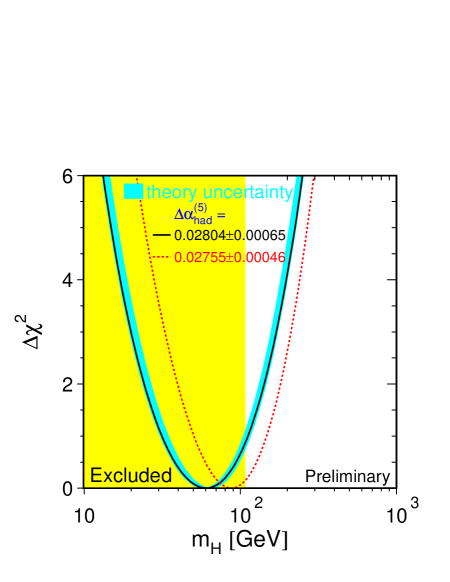
Figure 8: Constraint on $m_{H}$ from the precision observables, treating the standard model as a fundamental field theory. Status as of August 2000 [50].

As with any fit there are assumptions behind it. An important assumption behind Fig. 8 is to restrict the free parameters to the renormalizable couplings of the one-doublet Higgs model, which is equivalent to assuming $\Lambda_{\rm SM}\to\infty$. The bound on the Higgs mass suggested by the blue-band fit is now $m_{H}<170$ GeV at 95% (one-sided) confidence level [51] (and $m_{H}<270$ GeV at 99% CL). At high confidence, the fit would put the standard-model Higgs in the golden region with many measurable branching ratios. The combination of Figs. 7 and 8, which seem to imply that the real world is very like the standard model and that the Higgs is light, is sometimes used to argue that Higgs physics at the LC is nearly guaranteed to be extremely compelling.

There are two reasons to be careful about such an argument. First, the bound is brittle, because it is really a bound on $\log(m_{H}/m_{Z})$. Recent measurements from BES of the cross section for $e^{+}e^{-}\to{\rm hadrons}$, at $\sqrt{s}$ above and below the $\psi$ resonances, require a change in the treatment of the running of the electromagnetic coupling. After re-fitting, the bound on the Higgs mass appears to be several tens of GeV higher [51]. In a more qualitative vein, a few years ago the preferred ellipse was at somewhat lower $S$ and $T$. At that time the data required non-standard models with heavy Higgs to have a small, negative shift in $S$. Now the data allow also non-standard models with a small, positive shift in $T$.

A second, deeper reason to be suspicious of Fig. 8 is the omission of non-renormalizable interactions. From a modern understanding of field theory, the standard model is an effective field theory, valid up to a scale $\Lambda_{\rm SM}$. At energies above $\Lambda_{\rm SM}$, nature should be explained by a more profound field theory or, perhaps, string theory. At present there is no experimental information on $\Lambda_{\rm SM}$, although there are several competing theoretical ideas with $\Lambda_{\rm SM}$ in the range 0.25–5 TeV. (Examples of $\Lambda_{\rm SM}$ are the typical mass of the lowest-lying superpartners, or the scale at which composite structure of the Higgs is evident.)

It is worth emphasizing that the scale $\Lambda_{\rm SM}$ must be finite, and not simply because model-building theorists believe in grand unification or string theory. In the mid-to-late ’80s there was great interest in the high-energy limit of scalar field theories, such as the Higgs sector of the standard model. This is not an easy problem, because as the energy probed becomes higher, the self-couplings of scalar fields grow, and the problem becomes non-perturbative. The best work was done by those working at the interface of particle physics and mathematical physics [52]. To make a long story short, no way was found to take $\Lambda_{\rm SM}\to\infty$, unless the renormalized self-coupling vanishes in the limit. (This is the so-called “triviality” of scalar field theory, because there is no interaction at finite, physical energies.) On the other hand, a phenomenologically viable theory, with non-vanishing self-interaction and $m_{H}$, is obtained for finite $\Lambda_{\rm SM}$.

Once one accepts that $\Lambda_{\rm SM}$ is finite and unknown, the fits leading to the blue band must be redone, allowing higher-dimension (or non-renormalizable) interactions to float in the fit [53]. These contributions are suppressed by a factor of $(v/\Lambda_{\rm SM})^{2}$, or a higher power, where $v=246$ GeV is the Higgs field’s vacuum expectation value. Unless $\Lambda_{\rm SM}$ is close to $v$, these contributions are small, but today’s data are precise enough to notice them even if $\Lambda_{\rm SM}$ is as high as several TeV. It is easy to understand why they have been omitted for so long: when precision fits were first carried out, as seen in Fig. 7(b), the data just began to constrain radiative effects; power-suppressed contributions were in the noise. Now, however, the precision of the data is good enough to be sensitive to power corrections as well.

The omission of the higher-dimension interactions has been restored, in an essentially model-independent way, in at least three papers. Hall and Kolda [54] considered operators that would be induced by TeV-scale quantum gravity, and find that the bound is removed for $4~{}{\rm TeV}\mathop{\raisebox{-1.72218pt}{\hbox to0.0pt{$\sim$\hss}}\raisebox{1.72218pt}{$<$}}\Lambda_{\rm SM}\mathop{\raisebox{-1.72218pt}{\hbox to0.0pt{$\sim$\hss}}\raisebox{1.72218pt}{$<$}}11~{}{\rm TeV}$. Bagger, Falk, and Swartz [55] considered an effective field theory without a propagating Higgs field, which applies to models with Higgs mass also of order $\Lambda_{\rm SM}$ or with no Higgs boson at all. They found that the data are consistent with $\Lambda_{\rm SM}\mathop{\raisebox{-1.72218pt}{\hbox to0.0pt{$\sim$\hss}}\raisebox{1.72218pt}{$<$}}3$ TeV. (The precise definition of $\Lambda_{\rm SM}$ differs in the two frameworks, so there is no conflict between the inequalities.) Chivukula, Hölbling, and Evans [56] considered the renormalizable interactions of the standard model, plus interactions that contribute to $T$. The results of their fits are shown in Fig. 9.

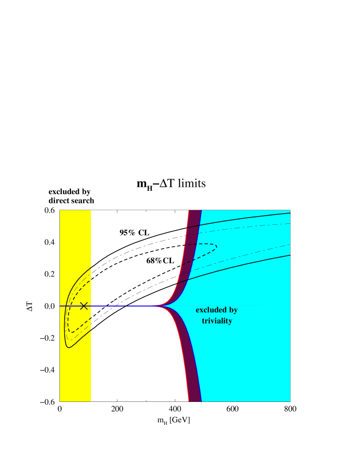
Figure 9: Constraint on $m_{H}$ and $T$. From Ref. [56]. The contours show the fit to precisely measured electroweak observables. The exclusion for low mass is from non-observation at LEP. In the region “excluded by triviality” many observables, not just those affecting $T$, would be expected to show non-standard effects at the per-mil level or higher, as discussed in the text.

One sees that for very high scales, the usual blue-band fit is recovered. If, however, $\Lambda_{\rm SM}$ is a few TeV, the data allow the Higgs mass to be large.

There is a simple model that exploits fully the weaker bounds that arise when treating the standard model as an effective field theory. If one adds to the standard model fields a vector-like quark with the $SU(3)_{C}\times SU(2)_{W}\times U(1)_{Y}$ quantum numbers of the right-handed top quark and a mass of a few TeV, the Higgs may have a mass significantly higher than the one inferred from Fig. 8 [57], as high as 1 TeV. This model is well motivated because it is an intermediate effective theory of the top-quark seesaw model [58], an explicit model of dynamically broken $SU(2)_{W}\times U(1)_{Y}$. Another example is provided by models with extra dimensions, in which the standard-model gauge bosons propagate in extra dimensions, while the fermions and Higgs boson are confined to four-dimensions. Then the fit to the electroweak data allows a Higgs mass of up to 500 GeV [59]. Finally, the radion, a particle that arises with warped extra dimensions, can cancel the Higgs’s contribution to $T$, again loosening the bounds [60].

When treating the standard model as an effective theory the experimental bounds seem not much tighter than theoretical bounds, based on triviality. The triviality bound is an extension of the unitarity bound. The latter anticipates either a physical Higgs resonance or a breakdown of tree-level unitarity in the $WW$ scattering amplitude below an energy of around 1 TeV [61]. Of course, in a real quantum field theory (and in nature) unitarity does not break down. The apparent breakdown at the tree level stems from a large Higgs self-coupling, so one should handle the full theory non-perturbatively. As mentioned above, this possibility has been studied extensively [52]. This analysis finds that either the Higgs mass is less than approximately 700 GeV, or decay vertices or scattering amplitudes exhibit deviations from the $\Lambda_{\rm SM}\to\infty$ limit at the percent level. The nuance of the result leads to other, equivalent conclusions: Fig. 9, for example, draws the bound on $m_{H}$ where the deviations would be at the per-mil level. On the other hand, the deviations could be of order one, but without any new resonances, yet $m_{H}\approx 1$ TeV. The present fits of data to the standard model with finite $\Lambda_{\rm SM}$ yield similar numbers, but the fits are stronger, because they close the loophole of “deviations at some level.”

The data-driven bound on the Higgs mass depends greatly on the scale $\Lambda_{\rm SM}$. The only insights into the value of this scale are theoretical, and the principal one is the fine-tuning problem. In general there are radiative corrections to the parameters of the standard model from virtual processes between the weak scale $v$ and $\Lambda_{\rm SM}$. In particular, the Higgs potential has a mass parameter $\mu^{2}<0$. The parameter in the effective theory is a sum,

$$\mu^{2}=\mu_{0}^{2}+c\Lambda_{\rm SM}^{2}\sum_{i}(\pm)_{i}g_{i}^{2},$$ (7)

of the tree-level $\mu_{0}^{2}$ plus contributions from loop processes. The constant $c$ depends on the underlying theory, the $g_{i}^{2}$ are couplings of the Higgs to particle $i$, and the sign is plus (minus) for bosons (fermions). If $g\Lambda_{\rm SM}$ is much larger than $\mu$, there is an unnatural fine-tuning problem. This is a serious issue, because some obvious choices for $\Lambda_{\rm SM}$ are the scale of gravity ($M_{\rm Planck}$) or of gauge-coupling unification ($\Lambda_{\rm GUT}$). Consequently, it is believed that $\Lambda_{\rm SM}$ is smaller: a few TeV, at most [62]. The best ideas for physics between $\Lambda_{\rm SM}$ and $\Lambda_{\rm GUT}$ (or $M_{\rm Planck}$) solve their own fine-tuning problem by some other means. For example, in supersymmetric models the supersymmetry requires the terms in the sum to cancel, for energies above the susy scale. With extra dimensions the unification scales need not be so high after all, 10-100 TeV, so the hierarchy of scales presents no problem. In any case, we note that the standard model’s fine-tuning problem is least severe when the scale $\Lambda_{\rm SM}$ is relatively low, but then the Higgs mass may be in the intermediate-mass or heavy regions.

3.5 Intermediate-mass Higgs Measurements

In the intermediate Higgs mass range, defined in this report to be the range from $2m_{W}$ to $2m_{t}$, the dominant decay is $H\to W^{+}W^{-}$. The branching fraction for this decay is a function of the weak coupling constant $g$ and kinematic constraints for on-shell $W$ bosons. Above $2m_{Z}$, the BR($H\to Z^{0}Z^{0}$) also becomes large, though smaller than BR($H\to W^{+}W^{-}$). Therefore, the most significant tests one can make in most of this mass range is whether the measured couplings of the Higgs boson to weak gauge bosons is in agreement with the Standard Model prediction. For the low end of this mass range ($m_{H}\mathop{\raisebox{-1.72218pt}{\hbox to0.0pt{$\sim$\hss}}\raisebox{1.72218pt}{$<$}}170$ GeV), there is also a possibility of measuring the $b\bar{b}$ coupling.

Our approach is a simple one. We assume that the detector design is adequate to identify decays of the type $Z^{0}\rightarrow e^{+}e^{-}$ and $Z^{0}\rightarrow\mu^{+}\mu^{-}$ with 80% efficiency. We then calculate the number of predicted $H\to W^{+}W^{-}$, $H\to Z^{0}Z^{0}$, $H\to b\bar{b}$ decays. For the measurements described below, we make the following assumptions:

• 250 fb^-1 of delivered luminosity

• $\sqrt{s}=500$ GeV

• Associated production of Higgs via the process $e^{+}e^{-}\rightarrow Z^{0}H$, followed by $Z^{0}\rightarrow e^{+}e^{-}$ or $Z^{0}\rightarrow\mu^{+}\mu^{-}$

• Identification of the Higgs events through the missing mass technique

We have constrained the sample to associated production to give a direct measurement of the branching ratios by measuring the number of Higgs events and the number of decay events in the same dataset, independent of luminosity measurements and cross section calculations. Extrapolations for other values of the luminosity should be straightforward.

3.5.1 Estimates of statistical uncertainties

In Fig. 10, we present the number of predicted

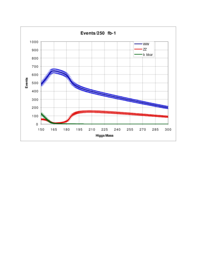
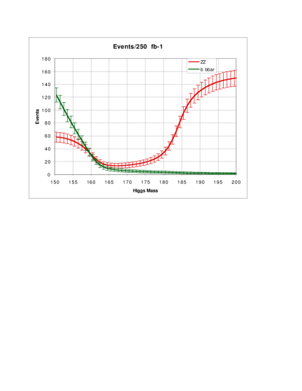
Figure 10: Number of events predicted for associated Higgs production with a center of mass energy of 500 GeV, 250 fb^-1 delivered luminosity, where the associated $Z^{0}$ is identified by decays into $e^{+}e^{-}$ or $\mu^{+}\mu^{-}$. (a) Number of $H\to W^{+}W^{-}$, $H\to Z^{0}Z^{0}$, and $H\to b\bar{b}$. (b) Blow-up of $H\to Z^{0}Z^{0}$ and $H\to b\bar{b}$ only.

$H\to W^{+}W^{-}$, $H\to Z^{0}Z^{0}$, and $H\to b\bar{b}$ events in 250 fb^-1 at $\sqrt{s}=500$ GeV. The cross section calculation for associated production comes from reference [63] and the branching ratios from the HDECAY program [15]. We have not included any additional decay branching fractions or identification efficiencies at this stage.

For reasonable expectations of $W$ identification efficiencies (50% or better) [64], we would expect to identify $\mathop{\raisebox{-1.72218pt}{\hbox to0.0pt{$\sim$\hss}}\raisebox{1.72218pt}{$>$}}$ 100 events over the entire mass range, with significantly more for $m_{H}$ in the region 150 GeV to 200 GeV. As a result, the statistical uncertainty on the measurement of BR($H\to W^{+}W^{-}$) will be $\mathop{\raisebox{-1.72218pt}{\hbox to0.0pt{$\sim$\hss}}\raisebox{1.72218pt}{$<$}}$ 10%.

The $Z^{0}$ and $b$ measurements are more problematic. In Fig. 10(b), we focus on the predicted number of events for $H\to Z^{0}Z^{0}$ and $H\to b\bar{b}$. Unless one is able to distinguish hadronic $Z^{0}$ decays from hadronic $W$ decays, it will be difficult to have adequate statistics to measure BR($H\to Z^{0}Z^{0}$) as the total number of $Z^{0}Z^{0}$ events is $\mathop{\raisebox{-1.72218pt}{\hbox to0.0pt{$\sim$\hss}}\raisebox{1.72218pt}{$<$}}$ 150 over the entire mass range. If one could identify one of the two $Z^{0}$’s in the Higgs decays (through leptons or $b\bar{b}$) 40% of the time, at best the statistical uncertainty of BR($H\to Z^{0}Z^{0}$) would be $\sim$ 11% for $m_{H}\sim$ 210 GeV. For $m_{H}<180$ GeV, the statistical uncertainties would be larger than 25%.

With this approach, the measurement of BR($H\to b\bar{b}$) with precision better than 25% will only be possible for $m_{H}\mathop{\raisebox{-1.72218pt}{\hbox to0.0pt{$\sim$\hss}}\raisebox{1.72218pt}{$<$}}160$ GeV. For larger masses, the branching fraction into $b\bar{b}$ is too small.

3.5.2 Different strategies for $Z\to b\bar{b}$

A center of mass energy of 500 GeV is not optimal for all Higgs masses in the range 150 GeV to 300 GeV. As can be seen in Fig. 11, the cross section for associated Higgs

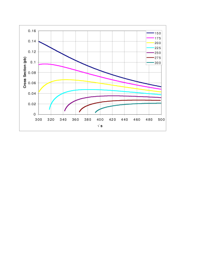
Figure 11: The cross section in pb^-1 for associated Higgs production vs. center of mass energy. The seven curves are for Higgs masses from 150 GeV to 300 GeV.

production depends upon both the Higgs mass and the center of mass energy. The peak value of the production cross section occurs at center of mass energy near $m_{H}+m_{Z}+50$ GeV. For the low end of the mass range ($\mathop{\raisebox{-1.72218pt}{\hbox to0.0pt{$\sim$\hss}}\raisebox{1.72218pt}{$<$}}175$ GeV), the production cross section is 2–2.5 times higher at $\sqrt{s}=300$ GeV than at the nominal energy $\sqrt{s}=500$ GeV.

As stated above, the measurement of $H\to b\bar{b}$ is statistics limited for the entire mass range. A possible approach to increase the statistics in this sample is to look for the $\nu\bar{\nu}$ decays of the associated $Z^{0}$, with the experimental signature being two tagged $b$s with mass consistent with the Higgs, along with significant missing energy from the two neutrinos. Since the BR($Z^{0}\to\nu\bar{\nu})$ is three times that of $e^{+}e^{-}$ plus $\mu^{+}\mu^{-}$, the gain extends the reach with 25% statistical uncertainty to $m_{H}\sim 165$ GeV. Another possibility would be to consider hadronic decays of the $Z^{0}$. This would require more detailed study, because mass reconstruction for both $Z$ and $H$ would have to be simulated. Finally, one should acknowledge that a measurement of a rare decay would come at the end of the Higgs phase of the LC program. Figure 12 shows the number of $ZH,\,Z\to l^{+}l^{-},\,H\to b\bar{b}$ events, and the resulting statistical error, in a long run of 2000 fb^-1, as a function of $m_{H}$ for several different possible running energies.

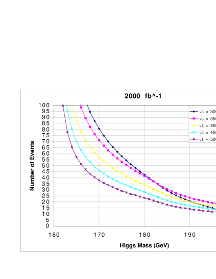
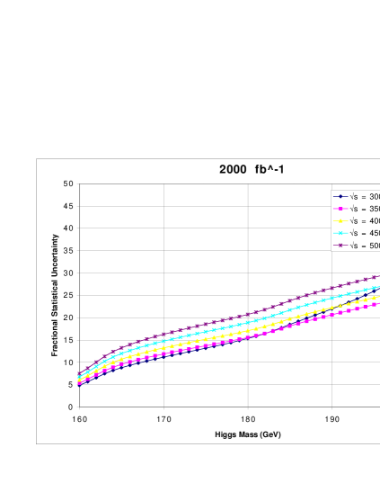
Figure 12: $ZH$ events in 2000 fb^-1 with $Z\to l^{+}l^{-}$ ($l=e,\mu$) and $H\to b\bar{b}$ vs. $m_{H}$. (a) Number of events. (b) Statistical error on BR($H\to b\bar{b}$). The five curves are for $\sqrt{s}$ from 300 GeV to 500 GeV.

Combining these strategies should, presumably, improve the prospects for this measurement.

3.6 Heavy Higgs Measurements

In this section we consider the contribution of an LC if the Higgs is heavy, $m_{H}>350$ GeV, and has standard-model couplings. As discussed above, such a heavy Higgs would require the existence of a non-standard effect; however, that effect could exist at a mass scale of several TeV, so that the heavy Higgs could possess couplings close to those of the standard model. For example, Ref. [57] found that the top-seesaw model can satisfy the electroweak constraints with a Higgs boson in this region, while the additional vector-like quark has mass above 1 TeV.

In this discussion, we assume that experiments at the LHC would discover this heavy Higgs, since a signal greater than 5$\sigma$ is claimed by both CMS [16] and ATLAS [17] for 30 fb^-1 for $350~{}{\rm GeV}<m_{H}\mathop{\raisebox{-1.72218pt}{\hbox to0.0pt{$\sim$\hss}}\raisebox{1.72218pt}{$<$}}1$ TeV. We ask what measurements an LC could contribute to better the understanding of a heavy Higgs boson.

We consider the specific case for $m_{H}~{}=500$ GeV and the Higgs has standard couplings. Then the standard-model width is calculated to be 70 GeV, and the branching ratios into the dominant decay modes are: 55% to $W^{+}W^{-}$, 25% to $Z^{0}Z^{0}$, and 20% to $t\bar{t}$.

At the LHC, the production cross section is 4 pb for $m_{H}~{}=500$ GeV. The decay of the Higgs into pairs of $Z^{0}$’s and the subsequent decay of the $Z^{0}$’s into either $e^{+}e^{-}$ or $\mu^{+}\mu^{-}$ gives a cross section times branching ratio into the four lepton final state, “$4\ell$” (the golden mode), of 3.2 fb. In 300 fb^-1, and assuming acceptance times efficiency to be 40%, the ATLAS TDR [17] states that 390 events in the golden mode can be used to measure the mass to a relative error better than 0.3%, the width to 6%, and the product of production cross section times branching ratio to 12%. (The last assumes a 10% uncertainty on the luminosity determination.) The LHC should be able to make a precision measurement on the ratio of branching ratios ${\rm BR}(H\to WW)/{\rm BR}(H\to ZZ)$. Other measurements, such as the $CP$ nature of the Higgs, are not discussed here.

Several measurements could potentially benefit from an LC. There is no obvious physics case that would require improving on LHC’s mass measurement. The machine with the largest usable statistics should be able to measure the width more precisely. At LHC, the measurement of the width comes from a direct fit of the data to the $4\ell$ lineshape, and its uncertainty is dominated by the statistical precision of the fit. The LC has a better chance of using the hadronic and neutrino decays of the two $Z$ bosons. The LHC appears unlikely to be able to make a precise measurement of $WWH$ and $ZZH$ couplings, due to both uncertainties in the normalization of luminosity and the lack of a sufficiently accurate value of the production cross section.

At an LC, the production of a very heavy Higgs requires both high energy and high luminosity. We consider running at $\sqrt{s}=800$ GeV with an integrated luminosity of 2500 fb^-1. At this energy, the production cross section of $H\nu\bar{\nu}$ dominates at 10 fb, but the production cross section of $HZ$ also contributes significantly at 6 fb. In all, approximately 40,000 Higgs would be produced. Even with such a glorious data set, the number of expected $4\ell$ candidates is only 46 events assuming 100% acceptance and efficiency and no backgrounds. We assume that in the case of an LC, the golden mode will not contribute to a high precision measurement due to limited statistics.

The expected sample that would be produced for Higgs decaying into $W^{+}W^{-}$ where either one or both $W$’s decay leptonically is 7,700 events. For Higgs decaying into $Z^{0}Z^{0}$, with at least one $Z^{0}$ decaying into a lepton pair ($e$ or $\mu$) and the other $Z^{0}$ decaying either into neutrinos or $b\bar{b}$, one expects 480 events. Other decay modes of the vector bosons appear to either have large backgrounds or have great difficulties in their reconstruction ($c$-tagging could help, for instance). Unlike the LHC, it is possible that the LC could observe and measure the branching ratio of Higgs into $t\bar{t}$. Final state modes that involve at least one lepton and two $b$-jets would provide a sample of 2750 events. Assuming that 10% of this sample is usable (within the acceptance, found efficiently over background, correctly $b$-tagged), the relative error on the branching ratio could be 6%. For a very heavy standard model-like Higgs, assuming that a sufficiently large data sample could be obtained, the LC could be the best place to measure the coupling of the Higgs to fermion pairs and, thus, explore the connection between fermion masses and electroweak symmetry breaking.

The last point is important, because a heavy Higgs with nearly standard couplings is almost certainly part of a larger sector, with other particles at higher mass. Then, while planning or awaiting an upgrade of the LC energy, it would be attractive to explore the underlying physics by running the LC in a “Giga$Z$” configuration [65]. By going beyond the current precision for the $Z$ lineshape and $W$ and top masses, one can pinpoint the allowable region in the $S$-$T$ plane and, thus, constrain theoretical models while gaining insight into the appropriate energy scale for new physics.

4 Extensions of the Standard Model

The fundamental particles observed so far are the gauge bosons of the $SU(3)_{C}\times SU(2)_{W}\times U(1)_{Y}$ symmetry group, the longitudinal degrees of freedom of the $W^{\pm}$ and $Z^{0}$, and three generations of quarks and leptons. Remarkably enough, there is a strong theoretical argument for the existence of further physical phenomena [61]: if the particles observed so far were the only existing ones, then the $WW$ scattering cross section would violate perturbative unitarity at a scale of order 1 TeV. Therefore, either the $W$ and $Z$ must have strongly coupled self-interactions at the TeV scale, or new fundamental degrees of freedom, beyond those observed so far, must exist. The scale of the new phenomena is within the reach of future collider experiments, and searching for them is a main goal of high-energy physics. In this section we discuss the known alternatives for these new phenomena, and their implications for experiments at an LC.

As discussed in Sec. 3, models with a Higgs boson, whether fundamental or composite, give a good description of all available data. Nevertheless, one should ask if there are phenomenologically viable models without a Higgs boson. At present it is not possible to reject such alternatives completely, because, as mentioned above, with no Higgs boson the self-interactions of the $W$ and $Z$ must become strong at the TeV scale. In that case one cannot use a loop expansion to compute the physical quantities relevant for comparing with the electroweak data. With our currently limited understanding of strongly-coupled field theories, it is hard to decide whether a theory without a Higgs boson can be viable.

Technicolor is a well-known class of theories of electroweak symmetry breaking without a Higgs boson [66]. Its defining feature is that the longitudinal degrees of freedom of the $W$ and $Z$ are composite states of some new fermions (called techni-fermions) bound by an asymptotically-free gauge interaction that confines below the TeV scale. If this interaction is similar to QCD, then one may use experimental data for hadrons to derive predictions. It turns out that the electroweak data impose a strict upper bound on the number of techni-fermions [47, 67]. Even for the minimal number of techni-fermions, it would be necessary that some additional interactions cancel in part the contributions of the techni-fermions to $S$. Therefore, QCD-like technicolor with many techni-fermions is an example of a theory without a Higgs boson that is ruled out. On the other hand, if the technicolor interaction is significantly different than QCD (e.g., if the scale-dependence of the technicolor coupling is very mild, a paradigm called “walking technicolor”), then one does not know how to test predictions of the theory against the data. Assuming that such a theory turns out to be viable and, indeed, realized in nature, its most important experimental test would be $WW$ scattering at energies of order 1 TeV. Such an experiment would reveal the strongly-coupled gauge boson interactions, potentially leading to the production of vector resonances or other bound states. The capability of an LC in this channel has been studied for several distinct models in the report for Snowmass ’96 [68]. Some technicolor models also allow the existence of light pseudo-scalar particles, which would be interesting to study at an LC.

Even though it may be conceivable that the Higgs boson does not exist, the impressive fit of the standard model to the experimental data may be taken as an indication for the existence of a Higgs boson. In the rest of this section we will assume that a Higgs boson indeed exists, the effective theory below a scale of a TeV being the standard model with the possible addition of other light states.

It is important to emphasize that even if the standard model proves to be the correct description of nature at energies up to a TeV or so, the standard model is at best a low-energy effective theory valid only up to some higher energy scale $\Lambda_{\rm SM}$. This statement is supported by a variety of arguments. In addition to the breakdown of scalar field theories, discussed in Sec. 3.4, there are two other robust arguments. The first is that the ${\rm U}(1)_{Y}$ gauge coupling also increases with energy, so this sector presumably also breaks down. The other is that the standard model does not include gravity. These problems could be resolved if $\Lambda_{\rm SM}$ is as large as the Planck scale ($M_{\rm Planck}\approx 2\times 10^{19}$ GeV), but it appears more likely that $\Lambda_{\rm SM}$ is in the TeV range or below. The reasoning is phrased in the literature in various forms, and it is often called the hierarchy problem. In its simplest form it boils down to the question of why the weak interactions are so much stronger than the gravitational interactions or, equivalently, why the electroweak scale $v=246$ GeV is so much smaller than the Planck scale. A theory which includes both the standard model and gravitational interactions should address this problem, together with the associated fine-tuning problem, Eq. (7). Broadly speaking, there are three classes of theories which attempt to solve the hierarchy problem:

• supersymmetric extensions of the standard model;

• theories of Higgs compositeness;

• theories with extra dimensions.

In each one of these classes of models there are new particles and interactions at a scale in the TeV range or below. In what follows we discuss these theories in turn.

4.1 Supersymmetric Extensions of the Standard Model

Supersymmetry (susy) is a space-time symmetry connecting fermions and bosons. In a certain well-defined sense, it is the largest space-time symmetry consistent with a unitary $S$-matrix [69]. It also arises in string theory, which is the leading candidate to unify gauge and gravitational forces. For these reasons, it offers an attractive theoretical framework for particle physics, whether or not it is directly relevant at the TeV scale.

Susy also has several features that make it the most popular extension of the standard model of electroweak symmetry breaking:

• Susy solves the fine-tuning aspect of hierarchy problem. The symmetry between particles of different spin (superpartners) leads to exact relations between diagrams containing loops of the respective superpartners. As a consequence, the quadratic radiative corrections to $\mu^{2}$ in Eq. (7) cancel.

• The minimal supersymmetric extension of the standard model (MSSM) offers tantalizing evidence that the gauge couplings of $SU(3)_{C}\times SU(2)_{W}\times U(1)_{Y}$ unify at a very high energy scale $\Lambda_{\rm GUT}$, on the order of $2\times 10^{16}$ GeV [70]. (This is often summarized as a prediction of $\sin^{2}\theta_{W}$.)

  The possibility that a simpler structure lurks behind the known gauge symmetries is extremely intriguing, with important implications, for example in proton decay experiments and in neutrino physics. Perhaps more importantly for collider phenomenology, gauge coupling unification in the MSSM works only if the spectrum of the new superpartners is within an order of magnitude of the TeV scale [71].

• In most phenomenologically viable models of low-energy supersymmetry one introduces a new conserved quantum number, $R$-parity, whose sole purpose is to forbid too rapid proton decay mediated by superpartners. In $R$-parity conserving theories the lightest superpartner (LSP) is stable and may be a suitable dark matter candidate. Its relic abundance varies greatly over parameter space, but nevertheless there are significant regions where the LSP relic density is of just the right size [72, 73].

These arguments only represent circumstantial evidence for supersymmetry. On the other hand, the simplest susy extensions have some troublesome features that one should bear in mind:

• The $\mu$ problem. Although susy protects the weak scale from large radiative corrections, there is still a potentially dangerous tree-level contribution to Eq. (7), which is allowed by all symmetries, including supersymmetry. The term $\mu_{0}^{2}$ on the right-hand side of Eq. (7) now consists of two contributions—a susy-breaking piece whose natural size is of the order of a TeV, and a susy-preserving piece, which is expected to be on the order of the fundamental new physics scale, e.g., the Planck scale. Hence, an uncomfortably large hierarchy remains. Various solutions to the $\mu$ problem have been claimed in the literature [74], but none seems to be very compelling.

• The susy flavor problem. Generic models suffer from severe problems associated with large flavor-changing effects. Without a dedicated suppression mechanism, the superpartners of the first two generations’ quarks and leptons must have masses as large as 100 TeV or higher [75].

• The proton decay problem. With the most general Yukawa-type couplings between quarks, leptons and their superpartners, the proton would decay too rapidly through susy-mediated processes. The simplest and most elegant solution to this problem is the imposition of $R$-parity (see above).

There is also a pragmatic reason to consider susy in detail from an experimental point of view. It offers a predictive, renormalizable and perturbatively calculable model with a wide variety of possible phenomenology. Study of the numerous possible signatures in susy models leads to a detector design that is well-suited to the observation of new physics, no matter what its origin. In the same sense, susy models are useful for comparing the physics capabilities of various future colliders, as they illustrate generic, yet disparate scenarios for new physics. More details can be found in the extensive literature—see, e.g., the whitepaper [1] or well-known reviews [76], and references therein.

4.1.1 Classification of susy models

A truly supersymmetric theory of particle physics would have only a few more parameters in addition to the standard ones. The interactions with gauge bosons and their superpartners (gauginos) are fixed by gauge symmetry and supersymmetry. Likewise, the couplings to Higgs bosons and their superpartners (higgsinos) are fixed by the observed fermion mass spectrum and supersymmetry. Of the few remaining parameters allowed by susy, some may be eliminated by other considerations, e.g., by imposing $R$-parity.

If exact, supersymmetry guarantees the degeneracy of the standard particles and their superpartners. Since this is not observed in nature, supersymmetry must be broken, and a model of TeV-scale physics must also have susy-breaking parameters. Unfortunately, there are too many parameters in general, and a completely systematic study is impractical. Hence, to make progress, one must make additional assumptions. One is on the field content. The minimal field content which includes the standard model fields is a model with two Higgs doublets, called the minimal supersymmetric standard model (MSSM). Consistent with supersymmetry and its theoretical motivations, it is, however, possible to have more fields, leading to non-minimal extensions (NMSSMs).

The number of free parameters can be reduced by assuming a mechanism for susy breaking. Typically this is achieved by postulating two sectors, a hidden sector, in which dynamical susy breaking takes place, and the sector in which we live. One then requires some mechanism to mediate the breaking of susy from the hidden sector to ours. The different options are known as

• gravity mediation, or supergravity (SUGRA) [77];

• gauge mediation, via standard [78] and/or non-standard [79] gauge interactions;

• anomaly mediation [80];

• gaugino mediation [81];

• Scherk-Schwarz susy breaking [82].

Rather than review the detailed features of the spectrum in each of these classes of models, we shall mention a few of the important distinctions below, when comparing the LHC and the LC physics reach and capabilities.

4.1.2 How does susy justify a linear collider?

In this subsection we present some arguments that make the case for an LC, in case low energy susy is connected to electroweak symmetry breaking. For this purpose, we outline the physics program needed to verify that susy has indeed been observed, and the specific ways in which an LC would help elucidate not only electroweak symmetry breaking but also supersymmetry breaking. We also contrast with the information gleaned from the LHC experiments.

A discovery of susy would mark the beginning of a golden era for particle physics. All known particles should have superpartners, with interactions and properties of their own. To confirm the picture experimentally one must [83]

1. prove that the new particles have the correct quantum numbers to be superpartners;

2. show that the couplings to gauge bosons and gauginos are equal (up to radiative corrections [84]), as predicted by supersymmetry;

3. show also that the couplings to Higgs bosons and higgsinos are related;

4. correctly identify the flavors of the squark and slepton resonances;

5. measure precisely the superpartners’ mass spectrum;

6. measure mixing angles of squarks, sleptons, charginos, and neutralinos;

7. combine the masses and mixing angles to extract the fundamental parameters of the Lagrangian.

If the superpartners in question are within the kinematic reach of an LC, then, on each of these seven counts, it can provide the most incisive information. In principle, an LC with high enough energy can produce the whole susy spectrum and can, thus, fully reconstruct the susy model.

The conventional wisdom is that the LHC is a discovery machine, while linear colliders are for precision studies. What this usually means is that the LHC can discover more particles, while the LC can measure their properties (masses, couplings, widths, quantum numbers etc.) better. Because of its higher parton center-of-mass energy, the LHC can certainly produce more species of particles than a LC in the 1 TeV range. But it is not at all certain that all of them can be observed at the LHC, because of the larger backgrounds. For example, observation of first and especially second generation squarks appears to be rather challenging at the LHC. On the one hand, one has to extract the squark signal under a much larger gluino signal. On the other hand, having extracted a squark signal, it appears rather difficult to show how many squark flavors are present. These questions have not been studied in great detail to date and deserve attention.

It is important to keep in mind that even if the LHC is able to observe more superpartners than the LC, the two sets do not necessarily coincide. Generically, the LHC does better for strongly interacting superpartners, while the LC does better for sleptons, charginos and neutralinos. In this way, the two machines complement each other.

It is often said that one should abandon susy as a key to electroweak physics, if the LHC does not observe it. But there are realizations of supersymmetry for which such a conclusion is unwarranted. It is easy to construct models, where discovering susy at the LHC is not at all straightforward. We give two examples for illustration. First, consider the following hierarchy of masses

$$m_{\tilde{g}}\gg m_{\tilde{q}}\sim m_{\tilde{\ell}}>m_{\tilde{h}}$$ (8)

where $m_{\tilde{g}}$, $m_{\tilde{q}}$, $m_{\tilde{\ell}}$ and $m_{\tilde{h}}$ are the masses of the gauginos, squarks, sleptons and higgsinos, respectively. Such a hierarchy can be typical of models based on Scherk-Schwarz susy breaking, with gauge fields in the bulk and chiral fields on the wall [85, 86]. If, furthermore, the gauginos are all heavy enough to be beyond the reach of the LHC, while all scalars are nearly degenerate, then the only observable signatures of susy come from slepton and squark pair production with subsequent two-body decays to higgsinos. The resulting dilepton plus missing energy signature has been analyzed [16] and the reach extends up to $m_{\tilde{\ell}}\sim 350$ GeV at most. A dijet signature, even if observable, is far from diagnostic of supersymmetry, and its appearance would elicit a number of alternative explanations. Second, there are also well-motivated susy models in which the dominant discovery signatures have many $\tau$ leptons. At the LC calorimetry can be used to detect hadronic decays of the $\tau$, whereas at at hadron machines the underlying event would tend to obscure them. Thus, in either of these scenarios the key discoveries could be left for an LC.

4.1.3 Contrast with LHC

Let us review some of the expectations for susy at the LHC. As long as the colored superpartners (gluino and squarks) are lighter than about $1$ TeV, strong production dominates and is not small compared to the QCD background. For the scenarios that have been under investigation, all with $M_{\rm susy}\leq 1$ TeV, the signal can be separated from the standard model backgrounds with simple cuts, yielding evidence for new particles and a rough estimate of the mass scale [87]. Next, one would examine the susy sample for special features. Depending on the particular model, one may be able to isolate specific decay chains and then use kinematic end points to determine combinations of masses, for example $\tilde{\chi}_{2}^{0}\to\tilde{\ell}\to\tilde{\chi}^{0}_{1}\to\tilde{G}$ in gauge-mediated models [88], or $\tilde{q}\to\tilde{\chi}^{0}_{2}\to\tilde{\ell}\to\tilde{\chi}^{0}_{1}$ in gravity mediated [89], anomaly-mediated [90] or string-inspired [91] models.

In summary, partial reconstruction of susy decay chains has been demonstrated for several sample cases, and this technique should extend to more generic cases. Moreover, experience from the Tevatron suggests that one should expect the LHC collaborations to achieve more with real data than in simulation. Nevertheless, a feature of the decay-chain method is that it yields mass differences, relative to the LSP mass, but the LSP mass itself is not well measured.

If an LC can produce at least one visible particle, it can be detected, and its decay can be used to measure the LSP mass. Then one could combine the LSP mass from the LC with the mass differences from the LHC to determine the spectrum with a precision that LHC alone would not have, and a kinematic reach that an LC (with $\sqrt{s}$ not larger than 1 TeV) would not have. One should note that in reconstruction of electroweak superpartners at an LC one can measure their masses precisely [92]. Even for squark mass measurements, an LC has an advantage because of the fixed center of mass energy, and squark masses can be measured with a precision of up to a few GeV [93].

It is easy to identify other advantages of linear colliders. First, consider the question of measuring the putative superpartners’ couplings. These can appear in two places: in production of superpartners, and in their subsequent decays. However, any particle with a mass of a few hundred GeV, and charged under any of the standard gauge interactions, decays promptly at the collision point. It is, thus, impossible to extract its couplings from a lifetime measurement. One can also consider ratios of branching ratios, but then at least one of the couplings has to be known by other means. At a hadron collider it may be difficult to disentangle all the different superpartner decays, since they are all simultaneously present. Therefore, the cleaner and more straightforward way to measure the couplings is through the production mechanism, i.e., from a cross-section measurement of direct sparticle production.

Even then, there are several complications. First, one has to extract events where the superpartners are being directly pair-produced, rather than appearing at the end of other particles’ decay chains. At the LHC, this typically reduces the discriminating power against standard-model backgrounds, and leads to smaller signal rates. For example, almost any susy model has a region of parameter space where the sleptons are lighter than the squarks or gluinos, and can be produced in cascade decays of those (colored) superpartners. Unfortunately, because of the relatively small slepton production cross section, the LHC can detect direct production of sleptons only up to $\sim 350$ GeV. The slepton reach gets significantly higher if indirect production from squark and gluino decays is also included, but this is of course not helpful for a slepton cross-section measurement.

There are several kinds of measurements that are much better suited to lepton than hadron machines. One arises when there is significant mixing between the scalar partners of the left- and right-handed fermions. In that case, to extract the coupling to the weak eigenstate, one must measure the mixing angle as well. Here, polarized beams give a unique advantage to lepton colliders. In many processes there is more than one intermediate state, and sometimes some of the virtual particles (usually $t$-channel) are either unknown or poorly measured. Beam polarization helps again, as one can enhance or suppress certain subprocesses. Quantum numbers of putative superpartners are most easily determined from the threshold behavior of sparticle pair production or angular distributions of decays, as discussed for the Higgs boson in Sec. 3.3. The well-defined energy and clean environment of an LC provide a clear edge over the LHC.

Another case where an LC is superior in disentangling the new physics, is when there are several superpartners that are roughly degenerate in mass. Some examples can be readily found in the existing susy models:

• The two heavy neutral Higgs boson states of the MSSM, the $CP$-even $H^{0}$ and the $CP$-odd $A^{0}$, can have a mass splitting below the experimental resolution of the LHC detectors.

• The mass splittings of higgsinos are typically on the order of a few GeV, because they are induced only by mixing effects in the chargino and neutralino mass matrices. Therefore, the decay products in higgsino transitions are extremely soft and unobservable at the LHC. But by carefully scanning through higgsino thresholds, an LC can measure the masses precisely.

• Sleptons and squarks from the first two generations must be nearly degenerate, to satisfy flavor-changing constraints.

A final piece of physics which can only be done at an LC is to elucidate the nature of a stable, neutral LSP. LSP pair production by itself does not give an observable signature, so one must either tag with an initial state photon, or consider associate production of the LSP and next-to-lightest neutralino. For an analysis as subtle as this one, the clean environment of an LC is crucial.

We should point out that experimental tests of the relations between the Higgs and higgsino couplings are extremely difficult at both the LHC and an LC. First, these tests can only be carried out for third-generation sfermions. Second, those couplings rarely appear in production processes, and their extraction from ratios of branching ratios appears to be difficult. Furthermore, the necessary decay channels must be open, which need not always be the case.

Let us comment on the optimum energy and luminosity. For the superpartners, energy is clearly a premium, because with higher energy a greater fraction of the spectrum is likely to be accessible. Until a superpartner is observed in an experiment, one can only guess the appropriate starting energy. In the next subsection, we shall discuss information from a variety of running or approved future experiments, both in particle physics and astrophysics, that may soon see some new signal. Nevertheless, it is likely that the full elucidation of susy will eventually require lepton colliders with $\sqrt{s}$ of a few TeV.

Once even a few superpartners are within its kinematic reach, an LC will provide physics information which is inaccessible at the LHC. High luminosity is then needed for better precision in measuring the fundamental parameters of the susy Lagrangian. In particular, with LC measurements one can start to unravel the mechanism of susy breaking. To do so, one needs the most important masses as precisely as possible. An important feature of an LC is its ability to perform threshold scans in energy. This leads to very precise determinations of the masses [92], and it becomes possible, without model assumptions, to distinguish among the susy breaking mechanisms listed above [94].

4.1.4 A glimpse into the future

If susy exists, how long do we have to wait to see the first hints of new physics? This question is especially important for LC planning, since the answer depends on how heavy the susy spectrum is and, therefore, has bearing on the required collider energy. With no experimental guidance, one has to rely on theoretical prejudice. The traditional avenue is to place upper limits on the superpartner masses based on naturalness arguments [95].

A more predictive, and somewhat better motivated, estimate can be made if one assumes that the LSP explains the missing non-baryonic dark matter in the universe. The LSP is then neutral and, hence, a mixture of an electroweak gaugino and a higgsino. Until recently, it was thought that only a gaugino-like LSP could be a good dark matter candidate. In that case one can derive model-dependent upper limits on the superpartner spectrum [96], with obvious implications for an LC. Recent work [72, 97] shows, however, that throughout a large portion of the (previously unexplored) parameter space, a mixed gaugino-higgsino neutralino state is also a perfectly good dark matter candidate. The possibility of a significant higgsino fraction has far-reaching consequences for current and near-future astrophysical searches, which look for traces of dark matter annihilation at the center of the Earth, Sun or our galaxy. As it turns out, before the LHC commences, the combination of all collider searches and both direct and indirect dark matter detection probes will map out all of the cosmologically preferred parameter space that is accessible to an LC with $\sqrt{s}=0.5$ TeV.

Figure 13 shows how this works in the case of minimal

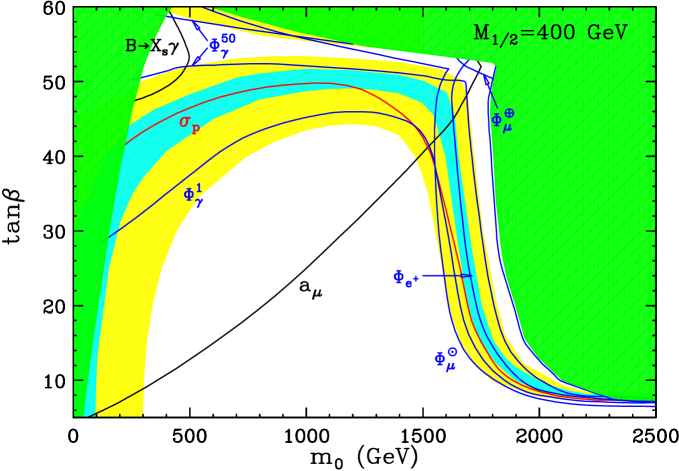
Figure 13: Estimated reach of various high-energy collider and low-energy precision searches (black), direct dark matter searches (red), and indirect dark matter searches (blue) before the LHC begins operation, for fixed $M_{1/2}=400$ GeV, $A_{0}=0$, and $\mu>0$. The signals considered are listed in the text. The projected sensitivities used for each experiment are given in Ref. [97]. The regions probed extend the curves toward the forbidden, green region. The regions with preferred (acceptable) LSP relic density are shaded in light blue (yellow).

supergravity [97], although the conclusion remains valid in other susy settings as well [98]. The cosmologically preferred (allowed) regions are shown in light blue (yellow). The green regions are excluded either by LEP or for theoretical reasons. The curves show the sensitivity limits of various experiments (the regions probed extend towards the excluded region). The signals considered are upward going muon flux from neutralino annihilation at the center of the Earth ($\Phi_{\mu}^{\oplus}$) and the Sun ($\Phi_{\mu}^{\odot}$); the continuum photon or positron flux from neutralino annihilation in our galaxy ($\Phi_{\gamma}$ and $\Phi_{e^{+}}$, respectively); direct dark matter detection in tabletop experiments ($\sigma_{P}$); and constraints from $B\to X_{s}\gamma$ and muon $g-2$. For illustration the gaugino mass parameter is chosen so that the chargino mass is roughly 250 GeV, barely within reach of a 500 GeV LC. But for lower gaugino masses, the sensitivity of the shown experiments is even better. We see that the combination of particle physics and astrophysical searches covers all the cosmologically interesting parameter space, and at least one is bound to observe a signal before the LHC begins operation. Conversely, if there is no hint of supersymmetry before that time, no superpartners will be within reach of a 0.5 TeV lepton collider (or dark matter would require another explanation).

4.1.5 Higgs properties in susy models

Since supersymmetry has a decoupling limit, most susy models have a light Higgs boson with nearly standard properties. As discussed in Sec. 3.2, precise measurements of this Higgs boson’s couplings could reveal its susy nature [26, 27]. In addition to this state, susy models have other, usually heavier Higgs boson states. By studying them one can measure the ratios of their vacuum expectation values, for example $\tan\beta$ in models with two doublets [101]. More details on heavy Higgs bosons can be found in the existing literature [102].

A new scenario [103], which was investigated during the Study, may arise in the simplest non-minimal extension, or NMSSM. The novel feature is the presence in the spectrum of light, mostly singlet, $CP$-odd scalars, which are called axions $A^{0}$. Their origin is easily understood as pseudo-Nambu-Goldstone bosons of an approximate, spontaneously broken global U(1) symmetry. The axions are, therefore, naturally light, because their mass is generated only by terms which explicitly break the symmetry. One then typically finds that the decay $h^{0}\to A^{0}A^{0}$, of the standard-model-like Higgs boson to a pair of axions, is kinematically allowed. A thorough study of the parameter space revealed that the branching fraction for this non-standard decay mode is typically on the order of $50\%$ and can compete with the conventional mode $h^{0}\to b\bar{b}$. Preliminary studies showed that the resulting Higgs boson signature $h^{0}\to 4b$ is marginally unobservable in Run II of the Tevatron (based on Run I efficiencies). At an LC, however, this decay should be easy to detect.

4.2 Non-supersymmetric Alternatives

In many discussions of physics beyond the standard model, electroweak symmetry is assumed either to be connected to supersymmetry or to be driven by strong dynamics, such as technicolor, without a Higgs boson. There is, however, a fertile middle ground of composite models. Here, typically, a strong binding mechanism accompanies, or drives, the breaking of electroweak symmetry, but some of the states have all the properties of a fundamental Higgs boson. Indeed, at sub-TeV energies these scenarios are often best described by a (possibly extended) Higgs sector, and the strong dynamics is apparent only above a TeV or so.

In this section, we review some features of such composite models in four dimensions, and more recent ideas inspired by the possibility of extra spatial dimensions. For completeness we include here other signals of extra dimensions that could be seen in linear colliders.

4.2.1 Higgs compositeness in four dimensions

The triviality of the Higgs sector in the standard model provides a new energy scale $\Lambda_{\rm SM}$. It may be called the compositeness scale, because at higher scales the Higgs boson is no longer a physical degree of freedom. Instead, some other fundamental degrees of freedom should become important. In the standard model with a light Higgs boson the compositeness scale is too high to be relevant for experiments. However, if there are new particles at the TeV scale, then the scale dependence of the Higgs couplings may be accelerated and the compositeness scale may be in the TeV range.

Composite models in which the Higgs field is made of some new fermions [104], or arises as a result of some new strong interactions involving the top quark [105, 106] have been extensively studied in the past. More recently, a class of models, called top-seesaw theory, in which a Higgs field appears as a bound state of the top quark with a new heavy quark, has proven phenomenologically viable and free of excessive fine-tuning [58, 107]. Furthermore, the top quark is naturally the heaviest standard fermion in these models, because it participates directly in the breaking of the electroweak symmetry. This theory has a decoupling limit, so at low energy it behaves as the standard model and, therefore, agrees with the electroweak data, as discussed in Sec. 3.4.

The interaction responsible for binding the Higgs field is provided by a spontaneously broken gauge symmetry, such as topcolor [108], or some flavor or family symmetry [109]. Note that such interaction is asymptotically free, allowing for a solution to the hierarchy problem. At the same time the interaction is non-confining, and therefore with a very different behavior than the confining technicolor interaction discussed at the beginning of this section.

Typically, in the top-quark seesaw theory the Higgs boson is heavy, with a mass of order 500 GeV [56]. However, the effective theory below the compositeness scale may include an extended Higgs sector, in which case the mixing between the $CP$-even scalars could bring the mass of the standard-model-like Higgs boson down to 100 GeV or so [107, 110]. One interesting possibility in this context is that there is a light Higgs boson with nearly standard couplings to fermions and gauge bosons, and nevertheless its decay modes are completely non-standard. This happens whenever, as in the NMSSM discussed in Sec. 4.1.5, a $CP$-odd scalar has a mass less than half the Higgs mass and the coupling of the Higgs to a pair of $CP$-odd scalars is not suppressed. The Higgs boson decays in this case into a pair of $CP$-odd scalars, each of them subsequently decaying into a pair of standard model particles, with model dependent branching fractions [111]. If the Higgs boson has standard model branching fractions, then the capability of an LC depends on $m_{H}$, as discussed in Sec. 3. On the other hand, if the Higgs boson has non-standard decays, an $e^{+}e^{-}$ collider may prove very useful in disentangling the composite nature of the Higgs boson, by measuring its width and branching fractions.

The heavy quark constituent of the Higgs has a mass of a few TeV while the gauge bosons associated with the strong interactions that bind the Higgs are expected to be even heavier. Above the compositeness scale there must be some additional physics that leads to the spontaneous breaking of the gauge symmetry responsible for binding the Higgs. This may involve new gauge dynamics [57], or fundamental scalars and supersymmetry. Evidently, an $e^{+}e^{-}$ collider could study these interesting strongly-interacting particles only if it operates at energies above a TeV.

Other models of Higgs compositeness have been proposed recently [112], and more are likely to be constructed in the future.

4.2.2 Theories with extra dimensions

In the last few years there has been an explosion of interest in models with extra spatial dimensions. We consider here several popular scenarios: large (i.e., mm-sized) extra dimensions for gravity only; TeV-sized extra dimensions accessible to some, but not all, standard particles; universal extra dimensions accessible to all particles; and warped extra dimensions, where the curvature of the extra dimensions plays a crucial role.

$\bullet$ Large extra dimensions

The recent intensive investigations of physics in extra dimensions has been sparked by the observation that the graviton could propagate in compact spatial dimensions as large as a millimeter [113]. As a result, the strength of gravity would be modified at short distances, so that the fundamental scale of quantum gravity could be in the TeV range, rather than $10^{19}$ GeV. This observation not only changes completely the nature of the hierarchy problem, but also leads to definite phenomenological predictions. The main implication is that there are Kaluza-Klein (KK) excitations of the graviton, i.e., spin-2 particles with universal couplings to matter, but suppressed by the Planck scale. The spectrum of KK gravitons is very dense, with spacings between states given by the inverse size of the extra dimensions. Although each of these states is very weakly coupled, the large number of states gives rise to large signals at energies comparable with the fundamental (TeV) scale.

In collider experiments the KK gravitons have two classes of effects: real KK graviton emission, characterized by missing transverse energy, and virtual KK graviton exchange, characterized by anomalous di-fermion or di-boson production at large invariant masses [114]. The current direct bounds on the scale of quantum gravity are of order 1 TeV and are set at the Tevatron [115] and at LEP [116]. More stringent bounds are set by the electroweak data, but these are model dependent and less robust.

Both the LHC and an LC with $\sqrt{s}=0.5$–1 TeV would be able to probe KK-graviton processes for fundamental scales up to several TeV. Moreover, if the scale of quantum gravity is indeed in this range, then collider experiments at $\sqrt{s}$ of several TeV would find phenomena which are well beyond any current theoretical understanding.

$\bullet$ TeV-size extra dimensions

Unlike the extra dimensions accessible only to gravity, which could be macroscopic, extra spatial dimensions accessible to standard model particles are constrained by Tevatron and LEP data to be smaller than of order $(1~{}{\rm TeV})^{-1}$. Nevertheless, the existence of TeV-size extra dimensions is a logical possibility, and is motivated by various theoretical considerations, such as the generation of hierarchical quark and lepton masses, or the potential for gauge coupling unification at a scale in the TeV range [117].

The immediate consequence of this scenario is the existence of towers of KK excitations for the particles that propagate in the TeV-size extra dimensions. For example, the gluons would have spin-1 color-octet excitations. Their masses are given by $\sqrt{j}/R$ where $R$ is the radius of the extra dimensions and $j$ is an integer that labels the KK level. The number of states on each level depends on the number of extra dimensions. Both the density of occupied levels and the average number of states ($D_{n}$) on a level increase with the number of extra dimensions, as can be seen in Table 4.

Table 4: The mass, $M_{n}$, and number of states, $D_{n}$, of the $n$th occupied KK level, for $\delta\leq 3$ extra dimensions, compactified on a torus. For illustration, only the first nine levels are shown here explicitly.

	$n$	$\;1\;$	2	3	4	5	6	7	8	$9$
$\delta=1$	$M_{n}R$	1	2	3	4	5	6	7	8	9
	$D_{n}$	2	2	2	2	2	2	2	2	2
$\delta=2$	$M_{n}R$	1	$\sqrt{2}$	2	$\sqrt{5}$	$\sqrt{8}$	3	$\sqrt{10}$	$\sqrt{13}$	4
	$D_{n}$	4	4	4	8	4	4	8	8	4
$\delta=3$	$M_{n}R$	1	$\sqrt{2}$	$\sqrt{3}$	2	$\sqrt{5}$	$\sqrt{6}$	$\sqrt{8}$	3	$\sqrt{10}$
	$D_{n}$	6	12	8	6	24	24	12	30	24

The $W,Z$ and photon would have color-singlet spin-1 excitations with a mass spectrum similar to the KK gluons, but slightly perturbed due to the electroweak symmetry breaking. In the popular case in which the quarks and leptons are localized on a three-dimensional domain wall (a 3-brane), the KK excitations of the gauge bosons have the same couplings, up to a factor of order one, as the corresponding standard model states. Therefore, the $Z$ and photon KK states may be produced in the $s$ channel in $e^{+}e^{-}$ collisions. At the same time, the KK excitations of the electroweak gauge bosons contribute at tree-level to the electroweak observables and, as a consequence, are constrained to lie above $\sim 4$ TeV, unless there are even more compensating effects. Standard-model quarks and leptons might propagate in extra dimensions, and for each of these chiral fermions there is a tower of vector-like fermions (i.e., four-component spinors with the left- and right-handed components carrying the same charges) with mass separations of order $1/R$.

The KK excitations of standard model particles can be produced at the LHC unless the inverse radius of the extra dimensions is above $\sim 6$ TeV. An LC with $\sqrt{s}=0.5$–1 TeV is unlikely to produce directly any of these KK excitations, but is very sensitive to their presence via virtual effects. It could, for example, provide evidence that a 4 TeV KK excitation of the $Z$ is accompanied by an almost degenerate KK excitation of the photon [118]. One should emphasize here that the observation of a signal in $e^{+}e^{-}$ collisions fitting the virtual effects of certain KK excitations would not prove that extra dimensions indeed exist. Instead, the virtual effects may very well be due to some other new heavy particles from a four-dimensional model (for example a collection of $Z^{\prime}$ bosons rather than KK excitations of the photon and $Z$). On the other hand, observation of a series of KK resonances, say in a multi-TeV LC, not only would establish the existence of extra dimensions, but also would determine the number of extra dimensions and their structure.

$\bullet$ Universal extra dimensions

A qualitatively distinct case is that all standard model particles propagate in extra dimensions. The KK number is then conserved at each vertex, so that the KK excitations may be produced only in groups of two or more. Hence, direct bounds from the Tevatron and LEP are significantly lower. Moreover, the KK states do not contribute at tree level to the electroweak observables. The current mass bounds on the first KK states are as low as 300 GeV for $\delta=1$ universal extra dimension, and in the range 400–800 GeV for $\delta=2$ [119].

These loose bounds make the universal extra dimensions particularly interesting for collider experiments. At $\sqrt{s}>600$ GeV, an LC could already pair-produce KK leptons, quarks and gauge bosons. One possibility is that the KK states decay outside the detector, so that the signal would be pairs of highly ionizing tracks. Alternatively, interactions that do not conserve momentum in the extra dimensions may allow the KK states to decay promptly into pairs of standard model particles.

$\bullet$ Warped extra dimensions

Another explanation for the observed weakness of gravitational interactions is given by the possibility that there is one extra dimension, and the graviton is localized on a 3-brane far from the 3-brane where our world of standard-model particles is localized [120]. On our 3-brane the wave function of the graviton is suppressed exponentially, and in this way the huge hierarchy between the electroweak and Planck scales is naturally induced. The graviton again has KK excitations, but these now have a certain non-uniform mass spectrum in the TeV range, and rather large couplings at the TeV scale. These spin-2 resonances would have a striking signal at any collider sufficiently energetic to produce them. Specific studies of these KK gravitons at the LHC and at an LC can be found in Ref. [121].

It may also be possible that some of the standard model fields propagate in the bulk of the extra dimensions, in which case spin-0 and 1 resonances with an interesting spectrum could be produced at the LHC and an LC [122].

4.2.3 Higgs boson properties in models with extra dimensions

The presence of extra dimensions and, more generally, of any new physics beyond the standard model, may affect searches for the Higgs boson in several ways:

• It may modify the rates for producing the Higgs boson in standard processes. For example, mixing in the Higgs sector of the MSSM typically suppresses the production cross section. Likewise, in models with large extra dimensions, or with warped extra dimensions, the Higgs boson mixes with the spin-0 component of the graviton [123].

• It may modify the branching ratios for the standard-model-like Higgs boson, e.g., by adding new possible decay channels (such examples are given in Sections 4.1.5 and 4.2.1), or through radiative corrections due to new particles (see, e.g., Ref. [124]).

• It may yield qualitatively new Higgs production mechanisms. For example, some flavor models in extra dimensions [125, 126] couple the standard Higgs boson to a bulk scalar (called a flavon) through non-renormalizable interactions. This may lead to the possibility of Higgs-flavon associated production at both hadron and lepton colliders [127]. The Higgs boson branching fractions are nearly standard, and the observed signature is $b\bar{b}\hbox to0.0pt{\,/\hss}E_{T}$. At the Tevatron and the LHC it is almost impossible to separate it from $Zh^{0}$, but a lepton collider would be able to reveal the presence of extra-dimensional physics.

Apart from these phenomenological implications, various new phenomena due to the extra dimensions shed a new light on the origin of electroweak symmetry breaking and fermion mass generation [125, 128, 117]. An interesting example is provided by the TeV-size extra dimensions. The KK excitations of the standard model gauge bosons and fermions give rise to a scalar bound state with the quantum numbers of the standard model Higgs doublet [129, 130]. The Higgs boson appears as a composite scalar with a combination of KK modes of the top-quark playing the role of constituents. This can be easily understood given that the KK excitations of the gluons and electroweak gauge bosons induce a strongly-coupled attractive interaction between the left- and right-handed top-quark fields.

Let us concentrate on a simple scenario, where all standard model gauge bosons and fermions (or at least the third generation of fermions) propagate in extra dimensions [130]. It is remarkable that out of the many possible bound states involving the quarks and leptons, the most deeply bound state has the quantum numbers of the Higgs doublet. Indeed, this state acquires a vacuum expectation value and, thus, breaks electroweak symmetry! Furthermore, this composite Higgs doublet has a large Yukawa coupling to the top-quark, which explains the large top mass. This is a direct consequence of the experimentally determined gauge charges of the quarks and leptons.

The framework that emerges here is very appealing. At a scale in the TeV range, called for convenience the string scale, $\Lambda_{s}$, the only degrees of freedom are the $SU(3)_{C}\times SU(2)_{W}\times U(1)_{Y}$ gauge bosons and the three generations of quarks and leptons, all of them propagating in a higher-dimensional spacetime. (At even higher energy scales, the fundamental degrees of freedom of a theory incorporating quantum gravity are expected to become relevant, such as the winding modes of string theory.) Below the scale $\Lambda_{s}$, fermion–anti-fermion pairs bind via the $SU(3)_{C}\times SU(2)_{W}\times U(1)_{Y}$ interactions. Then, below the scale $1/R<\Lambda_{s}$ that sets the size of the extra dimensions, the physics is described by an effective four-dimensional theory. This effective theory is the usual standard model, with the possible addition of a few other scalars, such as the heavy states of a two-Higgs-doublet model. (Interestingly enough, in the case of four extra dimensions there is also a potentially light bound-state with the quantum numbers of a bottom squark [130].)

As well as being a simple model consistent with all the experimental data, this framework is also predictive. The top mass is predicted with an uncertainty of about 20% and agrees well with the experimental value. The Higgs mass also is determined theoretically, and the result is a narrow range

$$165~{}{\rm GeV}<m_{H}<230~{}{\rm GeV}.$$ (9)

The correct prediction of the top mass and, more importantly, the prediction of the Higgs quantum numbers are unmatched by the standard model or its supersymmetric extensions. This model does suffer from some problems, which are, however, shared by the MSSM. It accommodates, but does not explain, the light quark and lepton masses. Also, a moderate tuning is required to keep the electroweak scale below $1/R$. A fuller comparison of the MSSM with this model of composite Higgs from extra dimensions can be found in Sec. 6 of Ref. [130]. Here we only add that in the case of universal extra dimensions the fine-tuning is no longer an issue because of the rather loose bound on $R$ ($1/R>400$–800 GeV for two extra dimensions).

A dedicated study of the signatures of the composite Higgs model from extra dimensions at the LHC and an LC has not yet been pursued. The prediction in Eq. (9) places the Higgs boson in the intermediate mass range, discussed in Sec. 3.5. More striking than the Higgs physics would be the non-standard phenomena discussed above. Eventually multi-TeV lepton collisions would be desired, to verify the layers of physics at the electroweak, compactification, and string scales.

5 Conclusions and Recommendations

Despite the success of the standard model of particle physics, we do not expect it to give a complete explanation of nature, at the very least because it does not incorporate gravity. At an aesthetic level, theorists expect gauge forces to unify with each other and with gravity, somewhere below the Planck mass. At a more concrete level, solid theoretical investigation of the “triviality problem” provides strong evidence that the scalar sector breaks down when applied to arbitrarily high energies. Consequently, the scalar (Higgs) sector is useful only if it is treated as an effective field theory, valid only up to some finite energy scale, $\Lambda_{\rm SM}$. Indeed, it is fair to call the $SU(3)_{C}\times SU(2)_{W}\times U(1)_{Y}$ gauge symmetry and the quarks’ and leptons’ quantum numbers, which all are here to stay, laws of nature. The scalar sector and interactions with it, on the other hand, merely represent a working model.

Above the scale $\Lambda_{\rm SM}$ new forms of matter are at play. The masses of quarks, charged leptons, and electroweak gauge bosons are generated by interactions with this matter. (These masses are otherwise forbidden by the electroweak gauge symmetry.) These interactions also lead to flavor and $CP$ violation, at least in the quark sector. Understanding this matter is thus a fundamental and central problem for physics. Despite the essential information that will come from hadronic collisions at the Tevatron and the LHC, it will take $e^{+}e^{-}$ (or $\mu^{+}\mu^{-}$) collisions at this scale to comprehend it fully. The most plausible scale for $\Lambda_{\rm SM}$ is around a TeV. This is not much higher than the scale of electroweak symmetry breaking, set by $v=(\sqrt{2}G_{F})^{-1/2}=246$ GeV. If $\Lambda_{\rm SM}$ were to be much higher, then $v$ would be unnaturally small compared to the mass scale of the agents of symmetry breaking.

Our ignorance of $\Lambda_{\rm SM}$ and of the form of the new matter make it both easy and difficult to argue in favor of a linear $e^{+}e^{-}$ collider with $\sqrt{s}=0.5$–1 TeV. The easy part is as follows. If $\Lambda_{\rm SM}$ is in the natural range, such an LC would start to explore many new states. The precise and model-independent mode of experimentation makes it likely that LC measurements would be able to diagnose the origin of electroweak symmetry breaking. If, alternatively, $\Lambda_{\rm SM}$ is (unnaturally) high, fits to precisely measured electroweak observables indicate that the lowest lying $CP$-even scalar—the Higgs boson—is light. Indeed, it is light enough for LC measurements to test the main features of mass generation in the standard model.

The hard part of the argument also stems from recognizing that the standard Higgs sector is, at best, an effective theory. Any list of measurements and, thus, their luminosity and energy requirements hinges on a scenario for the underlying physics. Many scenarios in the literature lead to an exciting program. Inevitably, others are less exciting. Nevertheless, the LC affords an excellent opportunity to complement the LHC in elucidating what breaks electroweak gauge symmetry.

For the Higgs boson, this report concentrates on scenarios that are close to the standard model. This is motivated mostly by the precise electroweak data. Models with a decoupling limit, by definition, can support a light Higgs with new states at high masses. They automatically satisfy constraints of the data in this and, typically, an adjacent neighborhood of parameter space. Within this neighborhood the phenomenology can change, and in some models the change may be drastic. More often than not, however, the potential of an LC becomes more interesting.

Another reason to consider nearly-standard Higgs bosons is that it gives two simple and reasonable scenarios for the Higgs program at LC. If the Higgs mass satisfies $m_{H}<2m_{W}$, then a detailed profile of the Higgs is measurable [25]. High luminosity is essential, because precisely measured branching ratios are sensitive to (possible) higher-mass Higgs bosons. Such a program should have an impact comparable to measurements of $Z$ boson properties at LEP and SLC. If $m_{H}>2m_{W}$ Higgs physics becomes more difficult: the decay to $b\bar{b}$ is rare and to $\tau^{+}\tau^{-}$ and $c\bar{c}$ are very rare. It is not yet clear how much integrated luminosity is needed for the rare modes, and without them the Higgs program is not quite as compelling. (If $m_{H}>2m_{t}$ the branching ratio to $t\bar{t}$ is large and measurable.) In non-supersymmetric extensions of the standard model such values of the Higgs mass are consistent with the precisely measured observables, because the Higgs boson’s contribution to them is small and could be compensated by similarly small contributions from TeV-scale particles. If the Higgs is indeed so heavy, then the flexibility of an LC to carry out the Giga$Z$ option (as well as improved measurements in $m_{W}$ and $m_{t}$) is attractive, because the indirect insights might help guide us to the next energy scale.

We also considered several extensions of the standard model—supersymmetry, compositeness and extra spatial dimensions—in which new physics resides at or below 1 TeV. Even with only a handful of accessible superpartners, an LC can perform many measurements complementary or superior to the LHC. Some of the most important are as follows: the precision on the mass of the lightest superpartner is expected to be only 10% at the LHC, but 1% at the LC. Direct studies of the slepton sector are a challenge at the LHC, but an LC can measure the masses, couplings and mixing parameters of the sleptons rather well. The well-defined center of mass energy of an LC is extremely helpful in resolving nearby resonances. We have even identified a case where the observation of supersymmetry at the LHC would remain ambiguous, and await confirmation elucidation at an LC. Moreover, linear colliders are also able to test definitively various supersymmetric relations and mass sum rules. In all cases, precision is needed for gaining insight into the underlying physics of supersymmetry breaking, and an LC of appropriate energy will be an essential tool to reach this goal.

There are several scenarios with extra spatial dimensions. The LC can help discriminate between them. For example, measurements of the mass spectrum of Kaluza-Klein (KK) modes can be used to determine the number of extra dimensions and their geometric structure. Even when the energy is not high enough to produce KK excitations directly, they can be exchanged as virtual particles. Thus, some information on the KK spectrum can be obtained by measuring scattering cross sections—in a way reminiscent of studying the $W$ boson in charged-current interactions, though not as much as in direct production.

These and other scenarios point to several features that a future $e^{+}e^{-}$ facility should have:

1. High (integrated) luminosity. Precision is desired for the couplings of the Higgs boson to the known particles. Indeed, in some cases, such as the Higgs self-coupling, or the $b\bar{b}$ coupling for $m_{H}>2m_{W}$, one must rely on rare processes. In susy and extra-dimension scenarios, there are also many other measurements to make, some requiring certain energies or particular combinations of beam polarization.

2. Polarization. At the electroweak scale and above, left- and right-handed fermions are fundamentally different. Choosing the right initial state, in response to the data, could prove vital. In susy, for example, polarization helps to pin down the quantum numbers of the superpartners, and it is the key that allows full exploration of the charginos and neutralinos.

3. Flexibility. Scans of the most important superpartner thresholds are valuable for deducing how supersymmetry is broken. In some other scenarios the Giga$Z$ program [65] is not merely interesting, but helpful for pointing to accelerators beyond the LHC and a 1 TeV LC. The $\gamma\gamma$ option can contribute to Higgs studies, and the $e^{-}e^{-}$ option is a good tool for studying the selectron, through $e^{-}e^{-}\to\tilde{e}^{-}\tilde{e}^{-}$.

4. Energy above 1 TeV. The TeV scale does not stop at $\sqrt{s}=1$ TeV, so energy upgrades are certainly crucial. The heavier superpartners may require $\sqrt{s}>1$ TeV; direct production of several resonances in a KK tower certainly does. It would be useful to understand how much of a sub-TeV layout could be reused for a multi-TeV LC.

The first three features appear in the NLC/JLC-X and TESLA designs, both of which are relatively mature. Higher energies appear to be upgrades (at least in length) or to await development of different technology, such as two-beam acceleration.

In the course of our study we addressed the experimental possibilities for a nearly-standard Higgs boson in the intermediate-mass and heavy regions. We also studied how angular distributions can be used to determine particles’ spin, particularly for the Higgs boson. On the theoretical side, we examined the connection of the LSP in susy to dark matter, and surveyed non-supersymmetric extensions of the standard model. There are a few questions that our studies have pointed to:

• Measurement of BR($H\to b\bar{b}$) for $m_{H}>2m_{W}$. We have attempted a first examination, using only $ZH$ events and then only leptonic $Z$ decays. How well, as function of $m_{H}$, can one do, when neutrino and hadronic $Z$ decays are added? When $\bar{\nu}H\nu$ production is included?

• Further simulations of spin determination. We have studied the Higgs and plan refinements. It would also be interesting to look at superpartners’ spins.

• Using light Higgs branching ratios to distinguish the standard model from non-standard models. Current studies have focussed on the MSSM and have omitted $CP$-violation.

• The decay $h/H\to AA\to b\bar{b}b\bar{b}$, which is allowed in an NMSSM and in certain composite models [111]. The LC looks promising, but a detailed study has not been done.

• Studies of benchmark scenarios in which susy remains obscure even in the light of LHC data. We have found examples either based on Scherk-Schwarz susy breaking or with $\tau$-rich final states.

Further issues will arise, as new theoretical ideas for physics at the TeV scale turn into testable scenarios, and as experiments yield more constraints and new surprises.

References

- [*] present address: Department of Physics, Yale University, New Haven, Connecticut
- [] present address: TH-Division, CERN, Geneva, Switzerland
- [1] J. Bagger et al. [American Linear Collider Working Group], “The case for a 500-GeV linear collider,” hep-ex/0007022.
-
[2]
“TESLA Technical Design Report Part III: Physics at an
linear collider,”
edited by R. D. Heuer, D. Miller, F. Richard, and P. Zerwas,
hep-ph/0106315,
http://tesla.desy.de/. - [3] T. Abe et al. [American Linear Collider Working Group], “Linear collider physics resource book for Snowmass 2001,” hep-ex/0106055, hep-ex/0106056, hep-ex/0106057, hep-ex/0106058.
- [4] S. Kuhlman et al. [NLC ZDR Design Group and NLC Physics Working Group], “Physics and technology of the Next Linear Collider: a report submitted to Snowmass ’96,” hep-ex/9605011.
-
[5]
N. Akasaka et al., “JLC Design Study,” KEK Report 97-1;
N. Toge, “JLC progress,” in Proceedings of the 20th International Linac Conference (Monterey, California, 21–25 August 2000), physics/0008172. -
[6]
R. Brinkmann,
“The TESLA linear collider,” to appear in
Proceedings of the 4th International Workshop on Linear Colliders
(Sitges, Spain, 28 April–5 May 1999),
DESY-TESLA-99-15;
R. Brinkmann [TESLA Collaboration], “TESLA linear collider design and R & D status,” in Proceedings of the 20th International Linac Conference (Monterey, California, 21–25 August 2000). - [7] R. W. Assmann et al., “A 3-TeV linear collider based on CLIC technology,” CERN-2000-008.
-
[8]
N. Walker,
“Status of the machine,”
talk at Hamburg meeting of the ECFA-DESY study,
http://www.desy.de/~ecfadesy/transparencies/, p. 14, and private communication. -
[9]
“TESLA Technical Design Report Part II: The Accelerator,”
edited by R. Brinkmann, K. Flöttmann, J. Roßbach,
P. Schmüser, N. Walker, and H. Weise,
http://tesla.desy.de/. - [10] “2001 report on the Next Linear Collider: A report to Snowmass 2001,” edited by N. Phinney [NLC Collaboration], FERMILAB-CONF-01/075-E, LBNL-PUB-47935, SLAC-R-571, UCRL-ID-144077.
-
[11]
M. Battaglia, “Higgs Physics at the linear collider:
Studies from the ECFA/DESY Working Group,”
talk at Fermilab Linear Collider Physics Study Meeting, 5 April 2000,
http://www-lc.fnal.gov/. -
[12]
T. Markiewicz, “NLC backgrounds: What’s new?” talk at the VIIIth International Workshop on Linear Colliders
(Frascati, Italy, 21–26 October 1999),
http://wwwsis.lnf.infn.it/lc99/Proceedings/table_of_contents.htm. -
[13]
M. Battaglia, “On the identification of
background overlapped on ”,
talk at Obernai meeting of the ECFA-DESY study,
http://ireswww.in2p3.fr/ires/ecfadesy/talks_sessions.html. - [14] M. Carena et al., “Report of the Tevatron Higgs working group,” hep-ph/0010338.
- [15] A. Djouadi, J. Kalinowski and M. Spira, Comput. Phys. Commun. 108, 56 (1998).
-
[16]
G. L. Bayatian et al. [CMS Collaboration],
Technical Proposal, CERN/LHCC 1994-038
(
http://cmsinfo.cern.ch/TP/TP.html). -
[17]
W. W. Armstrong et al.
[ATLAS Collaboration], Technical Design Report,
ATLAS-TDR-15,
CERN/LHCC 1999-015
(
http://atlasinfo.cern.ch/Atlas/GROUPS/PHY-SICS/TDR/access.html). - [18] N. Kauer, T. Plehn, D. Rainwater and D. Zeppenfeld, Phys. Lett. B503, 113 (2001).
- [19] D. Rainwater and D. Zeppenfeld, Phys. Rev. D60, 113004 (1999), E D61, 099901 (2000).
- [20] M. Dittmar and H. Dreiner, Phys. Rev. D55, 167 (1997); “ as the dominant SM Higgs search mode at the LHC for –180 GeV,” hep-ph/9703401.
- [21] D. Zeppenfeld, R. Kinnunen, A. Nikitenko and E. Richter-Wa̧s, Phys. Rev. D62, 013009 (2000).
- [22] O. J. Éboli and D. Zeppenfeld, Phys. Lett. B495, 147 (2000).
- [23] T. Plehn, D. Rainwater and D. Zeppenfeld, “Determining the structure of Higgs couplings at the LHC,” hep-ph/0105325.
-
[24]
A. Djouadi, W. Kilian, M. Mühlleitner and P. M. Zerwas,
Eur. Phys. J. C10, 45 (1999);
R. Lafaye, D. J. Miller, M. Mühlleitner and S. Moretti, “Double Higgs production at TeV colliders in the minimal supersymmetric standard model,” hep-ph/0002238. - [25] M. Battaglia and K. Desch, “Precision studies of the Higgs boson profile at the linear collider,” hep-ph/0101165.
- [26] M. Battaglia, “Measuring Higgs branching ratios and telling the SM from a MSSM Higgs boson at the linear collider,” to appear in Proceedings of the 4th International Workshop on Linear Colliders (Sitges, Spain, 28 April–5 May 1999), hep-ph/9910271.
- [27] M. Carena, H. E. Haber, H. E. Logan and S. Mrenna, “Distinguishing a MSSM Higgs boson from the SM Higgs boson at a linear collider,” hep-ph/0106116.
-
[28]
V. Drollinger and A. Sopczak,
“Comparison of Higgs boson mass and width determination of the LHC
and a linear collider,” Linear Collider Note LC-PHSM-2000-037,
http://www.desy.de/~lcnotes/notes.html. -
[29]
S. Dawson and L. Reina,
Phys. Rev. D57, 5851 (1998);
D59, 054012 (1999);
D60, 015003 (1999);
H. Baer, S. Dawson and L. Reina, Phys. Rev. D61, 013002 (2000). - [30] A. Juste and G. Merino, “Top-Higgs Yukawa coupling measurement at a linear collider,” to appear in Proceedings of the 4th International Workshop on Linear Colliders (Sitges, Spain, 28 April–5 May 1999), hep-ph/9910301.
- [31] D. J. Miller and S. Moretti, Eur. Phys. J. C13, 459 (2000); “The triple Higgs self-coupling at future colliders: a signal-to-background study for the standard model,” hep-ph/0001194.
-
[32]
P. Gay,
“Higgs self couplings at GeV,”
talk at Obernai meeting of the ECFA-DESY study,
http://ireswww.in2p3.fr/ires/ecfadesy/talks_sessions.html;
C. Castanier, P. Gay, P. Lutz and J. Orloff, “Higgs self-coupling measurement in collisions at center-of-mass energy of 500 GeV,” hep-ex/0101028. -
[33]
L. D. Landau, Dokl. Akad. Nauk Ser. Fiz. 60, 207 (1948);
C. N. Yang, Phys. Rev. 77, 242 (1950). - [34] J. J. Sakurai, Invariance principles and elementary particles, (Princeton University Press, 1964).
-
[35]
D. J. Miller, “Measurement of the Higgs boson spin in Higgsstrahlung,”
talk presented at the Linear Collider Workshop 2000
(Fermilab, October 24-28, 2000),
http://conferences.fnal.gov/lcws2000/web/david_miller_DESY/;
D. J. Miller, S. Y. Choi, B. Eberle, M. M. Mühlleitner, and P. M. Zerwas, Phys. Lett. B505, 149 (2001). - [36] V. Barger, K. Cheung, A. Djouadi, B. A. Kniehl and P. M. Zerwas, Phys. Rev. D49, 79 (1994). Note that one should redefine the angle in this paper’s Fig. 9 to for consistency with the right-handed coordinate system used in the formulae [P. M. Zerwas, private communication].
- [37] K. Hagiwara and M. L. Stong, Z. Phys. C62, 99 (1994).
- [38] T. Han and J. Jiang, Phys. Rev. D63, 096007 (2001).
- [39] K. Hagiwara, S. Ishihara, J. Kamoshita and B. A. Kniehl, Eur. Phys. J. C14, 457 (2000).
- [40] A. G. Akeroyd, A. Arhrib and M. Capdequi Peyranere, “Supersymmetric enhancement of associated production at colliders,” hep-ph/0104243; Mod. Phys. Lett. A14, 2093 (1999).
- [41] J. F. Gunion, H. E. Haber and C. Kao, Phys. Rev. D46, 2907 (1992).
-
[42]
A. Pilaftsis,
Phys. Rev. D58, 096010 (1998);
Phys. Lett. B435, 88 (1998);
A. Pilaftsis and C. E. M. Wagner, Nucl. Phys. B553, 3 (1999);
M. Carena, J. Ellis, A. Pilaftsis and C. E. M. Wagner, Nucl. Phys. B586, 92 (2000). - [43] J. F. Gunion and J. G. Kelly, Phys. Lett. B333, 110 (1994).
- [44] E. Asakawa, S. Y. Choi, K. Hagiwara and J. S. Lee, Phys. Rev. D62, 115005 (2000).
-
[45]
B. Grzadkowski, J. F. Gunion and J. Pliszka,
Nucl. Phys. B583, 49 (2000);
B. Grzadkowski, J. Pliszka and J. F. Gunion, “Measuring the relative -even and -odd Yukawa couplings of a Higgs boson at a muon collider Higgs factory,” hep-ph/0004034;
B. Grzadkowski, “Testing violation in the Higgs sector at muon colliders,” hep-ph/0005170. - [46] E. Asakawa, S. Y. Choi and J. S. Lee, Phys. Rev. D 63, 015012 (2001).
- [47] M. E. Peskin and T. Takeuchi, Phys. Rev. Lett. 65, 964 (1990); Phys. Rev. D46, 381 (1992).
- [48] M. L. Swartz, “Precision electroweak physics at the ,” in Proceedings of the XIXth International Symposium on Lepton and Photon Interactions at High Energies (August 9–14, 1999, Stanford), hep-ex/9912026.
-
[49]
D. M. Pierce and J. Erler,
Nucl. Phys. B Proc. Suppl. 62, 97 (1998);
J. Erler and D. M. Pierce, Nucl. Phys. B526, 53 (1998);
G. Cho and K. Hagiwara, Nucl. Phys. B574, 623 (2000). -
[50]
LEP Electroweak Working Group,
http://lepewwg.web.cern.ch/LEPEWWG/. -
[51]
B. Pietrzyk, “The global fit to electroweak data,”
talk at the XXXth International Conference on High Energy
Physics (July 27–August 2, 2000, Osaka, Japan),
http://ichep2000.hep.sci.osaka-u.ac.jp/. -
[52]
R. Dashen and H. Neuberger,
Phys. Rev. Lett. 50, 1897 (1983);
W. Langguth, I. Montvay and P. Weisz, Nucl. Phys. B277, 11 (1986);
M. Lüscher and P. Weisz, Nucl. Phys. B290, 25 (1987); B295, 65 (1988); B318, 705 (1989); Phys. Lett. B212, 472 (1988);
P. Hasenfratz and J. Nager, Z. Phys. C37, 477 (1988);
J. Kuti, L. Lin and Y. Shen, Phys. Rev. Lett. 61, 678 (1988);
A. Hasenfratz et al., Nucl. Phys. B317, 81 (1989);
U. M. Heller, M. Klomfass, H. Neuberger and P. Vranas, Nucl. Phys. B405, 555 (1993). - [53] R. S. Chivukula and N. Evans, Phys. Lett. B464, 244 (1999).
- [54] L. Hall and C. Kolda, Phys. Lett. B459, 213 (1999).
- [55] J. A. Bagger, A. F. Falk and M. Swartz, Phys. Rev. Lett. 84, 1385 (2000).
- [56] R. S. Chivukula, C. Hölbling and N. Evans, Phys. Rev. Lett. 85, 511 (2000).
- [57] H. Collins, A. Grant and H. Georgi, Phys. Rev. D61, 055002 (2000).
- [58] B. A. Dobrescu and C. T. Hill, Phys. Rev. Lett. 81, 2634 (1998).
- [59] T. G. Rizzo and J. D. Wells, Phys. Rev. D61, 016007 (2000).
- [60] C. Csaki, M. L. Graesser and G. D. Kribs, Phys. Rev. D63, 065002 (2001).
- [61] B. W. Lee, C. Quigg and H. B. Thacker, Phys. Rev. Lett. 38, 883 (1977); Phys. Rev. D16, 1519 (1977).
- [62] A quantitative analysis of the fine-tuning problem can be found in C. Kolda and H. Murayama, JHEP 0007, 035 (2000).
- [63] W. Kilian, M. Krämer and P. M. Zerwas, ‘Higgs-strahlung and vector boson fusion in collisions,” hep-ph/9605437.
- [64] R. Barate et al. [ALEPH Collaboration], Phys. Lett. B484, 205 (2000).
- [65] J. Erler, S. Heinemeyer, W. Hollik, G. Weiglein and P. M. Zerwas, Phys. Lett. B486, 125 (2000).
-
[66]
For recent reviews, see
K. Lane, “Technicolor 2000,” hep-ph/0007304;
R. S. Chivukula and J. Womersley, in “Review of particle physics,” D. E. Groom et al., Eur. Phys. J. C15, 1 (2000). -
[67]
B. Holdom and J. Terning,
Phys. Lett. B247, 88 (1990);
M. Golden and L. Randall, Nucl. Phys. B361, 3 (1991). - [68] T. L. Barklow et al., “Strong coupling electroweak symmetry breaking,” hep-ph/9704217.
- [69] R. Haag, J. T. Lopuszanski and M. Sohnius, Nucl. Phys. B88, 257 (1975).
- [70] S. Dimopoulos, S. Raby and F. Wilczek, Phys. Rev. D24, 1681 (1981).
-
[71]
P. H. Chankowski, Z. Pluciennik and S. Pokorski,
Nucl. Phys. B439, 23 (1995);
J. Bagger, K. Matchev and D. Pierce, Phys. Lett. B348, 443 (1995);
J. A. Bagger, K. T. Matchev, D. M. Pierce and R. Zhang, Phys. Rev. Lett. 78, 1002 (1997). - [72] J. L. Feng, K. T. Matchev and F. Wilczek, Phys. Lett. B482, 388 (2000).
-
[73]
J. Ellis, T. Falk, G. Ganis and K. A. Olive,
Phys. Rev. D62, 075010 (2000);
A. Bottino, F. Donato, N. Fornengo and S. Scopel, Phys. Rev. D62, 056006 (2000); D63, 125003 (2001). - [74] For a review see, e.g., N. Polonsky, “The parameter of supersymmetry,” hep-ph/9911329.
-
[75]
F. Gabbiani, E. Gabrielli, A. Masiero and L. Silvestrini,
Nucl. Phys. B477, 321 (1996);
J. A. Bagger, K. T. Matchev and R. Zhang, Phys. Lett. B412, 77 (1997). -
[76]
H. Murayama and M. E. Peskin,
Annu. Rev. Nucl. Part. Sci. 46, 533 (1996);
E. Accomando et al. [ECFA/DESY LC Physics Working Group], Phys. Rept. 299, 1 (1998). -
[77]
A. H. Chamseddine, R. Arnowitt and P. Nath,
Phys. Rev. Lett. 49, 970 (1982);
H. P. Nilles, Phys. Lett. B115, 193 (1982). -
[78]
M. Dine and A. E. Nelson,
Phys. Rev. D48, 1277 (1993);
M. Dine, A. E. Nelson and Y. Shirman, Phys. Rev. D51, 1362 (1995);
M. Dine, A. E. Nelson, Y. Nir and Y. Shirman, Phys. Rev. D53, 2658 (1996). -
[79]
R. N. Mohapatra and S. Nandi,
Phys. Rev. Lett. 79, 181 (1997);
B. A. Dobrescu, Phys. Lett. B403, 285 (1997);
H. Cheng, B. A. Dobrescu and K. T. Matchev, Phys. Lett. B439, 301 (1998); Nucl. Phys. B543, 47 (1999). -
[80]
L. Randall and R. Sundrum,
Nucl. Phys. B557, 79 (1999);
G. F. Giudice, M. A. Luty, H. Murayama and R. Rattazzi, JHEP 9812, 027 (1998). -
[81]
D. E. Kaplan, G. D. Kribs and M. Schmaltz,
Phys. Rev. D62, 035010 (2000);
Z. Chacko, M. A. Luty, A. E. Nelson and E. Ponton, JHEP 0001, 003 (2000). - [82] J. Scherk and J. H. Schwarz, Nucl. Phys. B153, 61 (1979); Phys. Lett. B82, 60 (1979).
- [83] J. L. Feng, M. E. Peskin, H. Murayama and X. Tata, Phys. Rev. D52, 1418 (1995).
-
[84]
K. Hikasa and Y. Nakamura,
Z. Phys. C70, 139 (1996);
H.-C. Cheng, J. L. Feng and N. Polonsky, Phys. Rev. D56, 6875 (1997); D57, 152 (1998);
M. M. Nojiri, D. M. Pierce and Y. Yamada, Phys. Rev. D57, 1539 (1998). -
[85]
I. Antoniadis, S. Dimopoulos, A. Pomarol and M. Quiros,
Nucl. Phys. B544, 503 (1999);
A. Delgado, A. Pomarol and M. Quiros, Phys. Rev. D60, 095008 (1999). - [86] H.-C. Cheng and K. T. Matchev, work in progress.
- [87] D. R. Tovey, Phys. Lett. B498, 1 (2001).
- [88] I. Hinchliffe and F. E. Paige, Phys. Rev. D60, 095002 (1999).
-
[89]
I. Hinchliffe, F. E. Paige, M. D. Shapiro, J. Söderqvist and W. Yao,
Phys. Rev. D55, 5520 (1997);
S. Abdullin et al. [CMS Collaboration], “Discovery potential for supersymmetry in CMS,” hep-ph/9806366;
H. Bachacou, I. Hinchliffe and F. E. Paige, Phys. Rev. D62, 015009 (2000);
I. Hinchliffe and F. E. Paige, Phys. Rev. D61, 095011 (2000);
M. M. Nojiri, D. Toya and T. Kobayashi, Phys. Rev. D62, 075009 (2000). - [90] F. E. Paige and J. Wells, “Anomaly mediated SUSY breaking at the LHC,” hep-ph/0001249.
- [91] B. C. Allanach, C. G. Lester, M. A. Parker and B. R. Webber, JHEP 0009, 004 (2000).
- [92] H. Martyn and G. A. Blair, “Determination of sparticle masses and SUSY parameters,” to appear in Proceedings of the 4th International Workshop on Linear Colliders (Sitges, Spain, 28 April–5 May 1999), hep-ph/9910416.
- [93] J. L. Feng and D. E. Finnell, Phys. Rev. D49, 2369 (1994).
- [94] G. A. Blair, W. Porod and P. M. Zerwas, Phys. Rev. D63, 017703 (2001).
-
[95]
R. Barbieri and G. F. Giudice,
Nucl. Phys. B306, 63 (1988);
G. W. Anderson and D. J. Castaño, Phys. Lett. B347, 300 (1995); Phys. Rev. D52, 1693 (1995);
L. Giusti, A. Romanino and A. Strumia, Nucl. Phys. B550, 3 (1999);
J. L. Feng, K. T. Matchev and T. Moroi, Phys. Rev. Lett. 84, 2322 (2000); Phys. Rev. D61, 075005 (2000). - [96] J. Ellis, G. Ganis and K. A. Olive, Phys. Lett. B474, 314 (2000).
- [97] J. L. Feng, K. T. Matchev and F. Wilczek, Phys. Rev. D63, 045024 (2001).
-
[98]
J. L. Feng,
talk at the Linear Collider Workshop 2000
(Fermilab, October 24–28, 2000),
http://conferences.fnal.gov/lcws2000/web/Jonathan_Feng/P023.html. - [99] H. N. Brown et al. [Muon Collaboration], Phys. Rev. Lett. 86, 2227 (2001).
-
[100]
J. L. Feng and K. T. Matchev,
Phys. Rev. Lett. 86, 3480 (2001);
L. L. Everett, G. L. Kane, S. Rigolin and L. Wang, Phys. Rev. Lett. 86, 3484 (2001). -
[101]
J. L. Feng and T. Moroi,
Phys. Rev. D56, 5962 (1997);
V. Barger, T. Han and J. Jiang, Phys. Rev. D63, 075002 (2001). -
[102]
A. Djouadi,
Int. J. Mod. Phys. A10, 1 (1995);
A. Djouadi, P. Ohmann, P. M. Zerwas and J. Kalinowski, “Heavy SUSY Higgs bosons at linear colliders,” hep-ph/9605437;
A. Djouadi, P. M. Zerwas and H. E. Haber, “Multiple production of MSSM neutral Higgs bosons at high-energy colliders,” hep-ph/9605437. - [103] B. A. Dobrescu and K. T. Matchev, JHEP 0009, 031 (2000).
-
[104]
D. B. Kaplan and H. Georgi,
Phys. Lett. 136B, 183 (1984);
D. B. Kaplan, H. Georgi and S. Dimopoulos, Phys. Lett. 136B, 187 (1984);
T. Banks, Nucl. Phys. B243, 125 (1984);
H. Georgi, D. B. Kaplan and P. Galison, Phys. Lett. 143B, 152 (1984);
H. Georgi and D. B. Kaplan, Phys. Lett. 145B, 216 (1984);
M. J. Dugan, H. Georgi and D. B. Kaplan, Nucl. Phys. B254, 299 (1985);
V. Koulovassilopoulos and R. S. Chivukula, Phys. Rev. D50, 3218 (1994). -
[105]
W. A. Bardeen, C. T. Hill and M. Lindner,
Phys. Rev. D41, 1647 (1990);
Y. Nambu, “BCS mechanism, quasi-supersymmetry, and fermion masses”, in the Proceedings of the XI Warsaw Symposium on Elementary Particle Physics, edited by Z. Ajduk, et al. (World Scientific, 1989); “Quasisupersymmetry, bootstrap symmetry breaking and fermion masses,” in the Proceedings of the 1988 International Workshop on New Trends in Strong Coupling Gauge Theories, edited by M. Bando, T. Muta and K. Yamawaki (World Scientific, 1989); “Bootstrap Symmetry Breaking In Electroweak Unification”, EFI-89-08 (1989);
V. A. Miransky, M. Tanabashi and K. Yamawaki, Mod. Phys. Lett. A4, 1043 (1989); Phys. Lett. B221, 177 (1989);
W. J. Marciano, Phys. Rev. Lett. 62, 2793 (1989). - [106] For a review, see G. Cvetic, Rev. Mod. Phys. 71, 513 (1999).
- [107] R. S. Chivukula, B. A. Dobrescu, H. Georgi and C. T. Hill, Phys. Rev. D59, 075003 (1999).
- [108] C. T. Hill, Phys. Lett. B266, 419 (1991).
- [109] G. Burdman and N. Evans, Phys. Rev. D59, 115005 (1999).
- [110] B. A. Dobrescu, Phys. Rev. D63, 015004 (2001).
- [111] B. A. Dobrescu, G. Landsberg and K. T. Matchev, Phys. Rev. D63, 075003 (2001).
- [112] H. Georgi and A. K. Grant, Phys. Rev. D63, 015001 (2001).
-
[113]
N. Arkani-Hamed, S. Dimopoulos and G. Dvali,
Phys. Lett. B429, 263 (1998);
I. Antoniadis, N. Arkani-Hamed, S. Dimopoulos and G. Dvali, Phys. Lett. B436, 257 (1998). -
[114]
G. F. Giudice, R. Rattazzi and J. D. Wells,
Nucl. Phys. B544, 3 (1999);
E. A. Mirabelli, M. Perelstein and M. E. Peskin, Phys. Rev. Lett. 82, 2236 (1999);
T. Han, J. D. Lykken and R. Zhang, Phys. Rev. D59, 105006 (1999);
J. L. Hewett, Phys. Rev. Lett. 82, 4765 (1999). - [115] B. Abbott et al. [D0 Collaboration], Phys. Rev. Lett. 86, 1156 (2001).
-
[116]
M. Acciarri et al., [L3 Collaboration],
Phys. Lett. B470, 281 (1999);
P. Abreu, et al., [DELPHI collaboration], Eur. Phys. J. C17, 53 (2000);
G. Abbiendi et al. [OPAL Collaboration], Eur. Phys. J. C18, 253 (2000);
R. Barate, et al., [ALEPH collaboration], “Single- and multi-photon production in collisions at centre-of-mass energies between 188.6 and 201.6 GeV,” ALEPH 2000-008, CONF-2000-005. - [117] K. R. Dienes, E. Dudas and T. Gherghetta, Nucl. Phys. B537, 47 (1999).
- [118] T. G. Rizzo, Phys. Rev. D61, 055005 (2000).
- [119] T. Appelquist, H. Cheng and B. A. Dobrescu, Phys. Rev. D64, 035002 (2001).
- [120] L. Randall and R. Sundrum, Phys. Rev. Lett. 83, 3370 (1999).
- [121] H. Davoudiasl, J. L. Hewett and T. G. Rizzo, Phys. Rev. Lett. 84, 2080 (2000).
- [122] H. Davoudiasl, J. L. Hewett and T. G. Rizzo, Phys. Rev. D63, 075004 (2001).
- [123] G. F. Giudice, R. Rattazzi and J. D. Wells, Nucl. Phys. B595, 250 (2001).
- [124] M. Carena, S. Mrenna and C. E. Wagner, Phys. Rev. D60, 075010 (1999).
- [125] N. Arkani-Hamed and S. Dimopoulos, “New origin for approximate symmetries from distant breaking in extra dimensions,” hep-ph/9811353.
- [126] N. Arkani-Hamed, L. Hall, D. Smith and N. Weiner, Phys. Rev. D61, 116003 (2000).
- [127] H.-C. Cheng and K. T. Matchev, Nucl. Phys. B563, 21 (1999).
-
[128]
N. Arkani-Hamed and M. Schmaltz,
Phys. Rev. D61, 033005 (2000);
Z. Berezhiani and G. Dvali, Phys. Lett. B450, 24 (1999). -
[129]
B. A. Dobrescu,
Phys. Lett. B461, 99 (1999);
H. Cheng, B. A. Dobrescu and C. T. Hill, Nucl. Phys. B589, 249 (2000). - [130] N. Arkani-Hamed, H.-C. Cheng, B. A. Dobrescu and L. J. Hall, Phys. Rev. D62, 096006 (2000).