Abstract

Based on a sample of four million events collected by ALEPH from 1991 to 1995, a measurement of the forward-backward asymmetry in $Z\rightarrow b\bar{b}$ decays using inclusive final states is presented. High-performance tagging of $b\bar{b}$ events in a wide angular range is achieved using neural network techniques. An optimal hemisphere charge estimator is built by merging primary and secondary vertex information, leading kaon identification and jet charge in a neural network. The average charge asymmetry, the flavour tagging efficiencies and mean $b$-hemisphere charges are measured from data and used to extract the pole $b$ asymmetry in the Standard Model

$$A^{0,b}_{\rm FB} = 0.1009\,\pm\,0.0027\,(stat)\,\pm\,0.0012\,(syst)\,,$$

corresponding to a value of the effective weak mixing angle of

${\rm sin^{2}}\theta_{\rm W}^{\rm eff}\>=\>0.23193\pm 0.00056$  .

submitted to Eur. Phys. J. C

The ALEPH Collaboration

A. Heister, S. Schael

Physikalisches Institut das RWTH-Aachen, D-52056 Aachen, Germany

R. Barate, I. De Bonis, D. Decamp, C. Goy, J.-P. Lees, E. Merle, M.-N. Minard, B. Pietrzyk

Laboratoire de Physique des Particules (LAPP), IN²P³-CNRS, F-74019 Annecy-le-Vieux Cedex, France

S. Bravo, M.P. Casado, M. Chmeissani, J.M. Crespo, E. Fernandez, M. Fernandez-Bosman, Ll. Garrido,¹⁵ E. Graugés, M. Martinez, G. Merino, R. Miquel,²⁷ Ll.M. Mir,²⁷ A. Pacheco, H. Ruiz

Institut de Física d’Altes Energies, Universitat Autònoma de Barcelona, E-08193 Bellaterra (Barcelona), Spain⁷

A. Colaleo, D. Creanza, M. de Palma, G. Iaselli, G. Maggi, M. Maggi, S. Nuzzo, A. Ranieri, G. Raso,²³ F. Ruggieri, G. Selvaggi, L. Silvestris, P. Tempesta, A. Tricomi,³ G. Zito

Dipartimento di Fisica, INFN Sezione di Bari, I-70126 Bari, Italy

X. Huang, J. Lin, Q. Ouyang, T. Wang, Y. Xie, R. Xu, S. Xue, J. Zhang, L. Zhang, W. Zhao

Institute of High Energy Physics, Academia Sinica, Beijing, The People’s Republic of China⁸

D. Abbaneo, P. Azzurri, G. Boix,⁶ O. Buchmüller, M. Cattaneo, F. Cerutti, B. Clerbaux, G. Dissertori, H. Drevermann, R.W. Forty, M. Frank, T.C. Greening,²⁹ J.B. Hansen, J. Harvey, P. Janot, B. Jost, M. Kado, P. Mato, A. Moutoussi, F. Ranjard, L. Rolandi, D. Schlatter, O. Schneider,² W. Tejessy, F. Teubert, E. Tournefier,²⁵ J. Ward

European Laboratory for Particle Physics (CERN), CH-1211 Geneva 23, Switzerland

Z. Ajaltouni, F. Badaud, A. Falvard,²² P. Gay, P. Henrard, J. Jousset, B. Michel, S. Monteil, J-C. Montret, D. Pallin, P. Perret, F. Podlyski

Laboratoire de Physique Corpusculaire, Université Blaise Pascal, IN²P³-CNRS, Clermont-Ferrand, F-63177 Aubière, France

J.D. Hansen, J.R. Hansen, P.H. Hansen, B.S. Nilsson, A. Wäänänen

Niels Bohr Institute, DK-2100 Copenhagen, Denmark⁹

A. Kyriakis, C. Markou, E. Simopoulou, A. Vayaki, K. Zachariadou

Nuclear Research Center Demokritos (NRCD), GR-15310 Attiki, Greece

A. Blondel,¹² G. Bonneaud, J.-C. Brient, A. Rougé, M. Rumpf, M. Swynghedauw, M. Verderi, H. Videau

Laboratoire de Physique Nucléaire et des Hautes Energies, Ecole Polytechnique, IN²P³-CNRS, F-91128 Palaiseau Cedex, France

V. Ciulli, E. Focardi, G. Parrini

Dipartimento di Fisica, Università di Firenze, INFN Sezione di Firenze, I-50125 Firenze, Italy

A. Antonelli, M. Antonelli, G. Bencivenni, G. Bologna,⁴ F. Bossi, P. Campana, G. Capon, V. Chiarella, P. Laurelli, G. Mannocchi,⁵ F. Murtas, G.P. Murtas, L. Passalacqua, M. Pepe-Altarelli,²⁴ P. Spagnolo

Laboratori Nazionali dell’INFN (LNF-INFN), I-00044 Frascati, Italy

A.W. Halley, J.G. Lynch, P. Negus, V. O’Shea, C. Raine, A.S. Thompson

Department of Physics and Astronomy, University of Glasgow, Glasgow G12 8QQ,United Kingdom¹⁰

S. Wasserbaech

Department of Physics, Haverford College, Haverford, PA 19041-1392, U.S.A.

R. Cavanaugh, S. Dhamotharan, C. Geweniger, P. Hanke, G. Hansper, V. Hepp, E.E. Kluge, A. Putzer, J. Sommer, K. Tittel, S. Werner,¹⁹ M. Wunsch¹⁹

Kirchhoff-Institut für Physik, Universität Heidelberg, D-69120 Heidelberg, Germany¹⁶

R. Beuselinck, D.M. Binnie, W. Cameron, P.J. Dornan, M. Girone,¹ N. Marinelli, J.K. Sedgbeer, J.C. Thompson¹⁴

Department of Physics, Imperial College, London SW7 2BZ, United Kingdom¹⁰

V.M. Ghete, P. Girtler, E. Kneringer, D. Kuhn, G. Rudolph

Institut für Experimentalphysik, Universität Innsbruck, A-6020 Innsbruck, Austria¹⁸

E. Bouhova-Thacker, C.K. Bowdery, A.J. Finch, F. Foster, G. Hughes, R.W.L. Jones,¹ M.R. Pearson, N.A. Robertson

Department of Physics, University of Lancaster, Lancaster LA1 4YB, United Kingdom¹⁰

I. Giehl, K. Jakobs, K. Kleinknecht, G. Quast, B. Renk, E. Rohne, H.-G. Sander, H. Wachsmuth, C. Zeitnitz

Institut für Physik, Universität Mainz, D-55099 Mainz, Germany¹⁶

A. Bonissent, J. Carr, P. Coyle, O. Leroy, P. Payre, D. Rousseau, M. Talby

Centre de Physique des Particules, Université de la Méditerranée, IN²P³-CNRS, F-13288 Marseille, France

M. Aleppo, F. Ragusa

Dipartimento di Fisica, Università di Milano e INFN Sezione di Milano, I-20133 Milano, Italy

A. David, H. Dietl, G. Ganis,²⁶ K. Hüttmann, G. Lütjens, C. Mannert, W. Männer, H.-G. Moser, R. Settles, H. Stenzel, W. Wiedenmann, G. Wolf

Max-Planck-Institut für Physik, Werner-Heisenberg-Institut, D-80805 München, Germany

J. Boucrot,¹ O. Callot, M. Davier, L. Duflot, J.-F. Grivaz, Ph. Heusse, A. Jacholkowska,²² J. Lefrançois, J.-J. Veillet, I. Videau, C. Yuan

Laboratoire de l’Accélérateur Linéaire, Université de Paris-Sud, IN²P³-CNRS, F-91898 Orsay Cedex, France

G. Bagliesi, T. Boccali, G. Calderini, L. Foà, A. Giammanco, A. Giassi, F. Ligabue, A. Messineo, F. Palla, G. Sanguinetti, A. Sciabà, G. Sguazzoni, R. Tenchini,¹ A. Venturi, P.G. Verdini

Dipartimento di Fisica dell’Università, INFN Sezione di Pisa, e Scuola Normale Superiore, I-56010 Pisa, Italy

G.A. Blair, G. Cowan, M.G. Green, T. Medcalf, A. Misiejuk, J.A. Strong, P. Teixeira-Dias, J.H. von Wimmersperg-Toeller

Department of Physics, Royal Holloway & Bedford New College, University of London, Egham, Surrey TW20 OEX, United Kingdom¹⁰

R.W. Clifft, T.R. Edgecock, P.R. Norton, I.R. Tomalin

Particle Physics Dept., Rutherford Appleton Laboratory, Chilton, Didcot, Oxon OX11 OQX, United Kingdom¹⁰

B. Bloch-Devaux,¹ P. Colas, S. Emery, W. Kozanecki, E. Lançon, M.-C. Lemaire, E. Locci, P. Perez, J. Rander, J.-F. Renardy, A. Roussarie, J.-P. Schuller, J. Schwindling, A. Trabelsi,²¹ B. Vallage

CEA, DAPNIA/Service de Physique des Particules, CE-Saclay, F-91191 Gif-sur-Yvette Cedex, France¹⁷

N. Konstantinidis, A.M. Litke, G. Taylor

Institute for Particle Physics, University of California at Santa Cruz, Santa Cruz, CA 95064, USA¹³

C.N. Booth, S. Cartwright, F. Combley,⁴ M. Lehto, L.F. Thompson

Department of Physics, University of Sheffield, Sheffield S3 7RH, United Kingdom¹⁰

K. Affholderbach,²⁸ A. Böhrer, S. Brandt, C. Grupen, A. Ngac, G. Prange, U. Sieler

Fachbereich Physik, Universität Siegen, D-57068 Siegen, Germany¹⁶

G. Giannini

Dipartimento di Fisica, Università di Trieste e INFN Sezione di Trieste, I-34127 Trieste, Italy

J. Rothberg

Experimental Elementary Particle Physics, University of Washington, Seattle, WA 98195 U.S.A.

S.R. Armstrong, K. Cranmer, P. Elmer, D.P.S. Ferguson, Y. Gao,²⁰ S. González, O.J. Hayes, H. Hu, S. Jin, J. Kile, P.A. McNamara III, J. Nielsen, W. Orejudos, Y.B. Pan, Y. Saadi, I.J. Scott, J. Walsh, Sau Lan Wu, X. Wu, G. Zobernig

Department of Physics, University of Wisconsin, Madison, WI 53706, USA¹¹

1 Introduction

The measurements of the forward-backward asymmetry of $b$-quarks from $e^{+}e^{-}\rightarrow Z\rightarrow b\bar{b}$ production offer the most precise determination of the weak mixing angle at LEP. This gives a sensitive test of Standard Model [1] predictions of electroweak radiative corrections and hence constrain the allowed range of the Higgs boson mass.

The polar angle distribution of the $b$-quark in the $e^{+}e^{-}\rightarrow Z\rightarrow b\bar{b}$ process is forward-backward asymmetric:

$$\frac{d\sigma_{b\bar{b}}}{d\cos\theta_{b}}\>=\>\sigma_{b\bar{b}}\,\frac{3}{8}\,\left(1+\cos^{2}\theta_{b}+\frac{8}{3}A^{b}_{\rm FB}\cos\theta_{b}\right)\,,$$

where $\theta_{b}$ is the angle between the incoming electron and the outgoing $b$-quark. In this paper an improved measurement of $A_{\rm FB}^{b}$ using inclusive $b$-hadron decays is presented, based on the data sample recorded by ALEPH on the $Z$ from 1991 to 1995. The analysis takes advantage of a reprocessing of LEP I data with improved charged particle tracking and of neural network techniques making maximum use of the available event information.

The method of selecting events containing $b\bar{b}$ quark pairs is upgraded with respect to the previous analysis [2]. The $b$-tagging algorithm based on the impact parameters of charged particle tracks is complemented with information from displaced secondary vertices, event shape variables and lepton identification. This leads to a 15% reduction of the statistical uncertainty. The estimate of the $b$-quark direction is based upon the hemisphere charge method [3], but also incorporates information from fast kaon tagging and separated primary and secondary vertex charge estimators. The fraction of incorrect charge tags is reduced by 10% with respect to the previous measurement, implying a 20% further reduction of the statistical uncertainty. Another new feature is the control of systematic uncertainties by use of double tag methods for both flavour and charge tags, which yields a reduction of the systematic uncertainty by about a factor of two.

Although lepton identification is used to select events in the $b$-tag algorithm, no use is made in the hemisphere charge method of the lepton beyond that of an ordinary charged track in the detector. This reduces the correlation with the forthcoming ALEPH $A_{\rm FB}^{b}$ analysis based on semileptonic final states.

2 The method

The measurement of $A^{b}_{\rm FB}$ requires knowledge of the direction of the $b$-quark from $Z\rightarrow b\bar{b}$ decay. The quark-antiquark axis is estimated using the reconstructed thrust axis, the direction of which is given throughout this paper by a positive value for the cosine of the thrust polar angle, $\cos\theta$. Each event is then divided into two hemispheres, F and B, by a plane perpendicular to the thrust axis. The forward hemisphere, F, is defined as the one into which the incoming electron points. The F-B orientation of the $b$-quark is determined on a statistical basis by estimating the hemisphere charges.

Hemisphere charges, $Q_{\mathrm{F}}$ and $Q_{\mathrm{B}}$, are formed using a neural network designed to optimise the separation power between $b$- and $\bar{b}$-quarks. The neural network also performs well for lighter quark flavours, albeit not in an optimal way. A forward-backward asymmetry for flavour $f$ at a given value of $\cos\theta$ is then proportional to the mean charge flow, $\langle Q_{\rm FB}^{f}\rangle$, between forward and backward hemispheres in pure $f\bar{f}$ events :

$$\langle Q_{\mathrm{F}B}^{f}\rangle = \langle Q_{\mathrm{F}}^{f}-Q_{\mathrm{B}}^{f}\rangle$$ (1)

$$= \frac{1}{n^{f}_{\rm tot}}\,\left(n^{f}_{\rm F}\langle Q_{f}-Q_{\bar{f}}\rangle+n^{f}_{\rm B}\langle Q_{\bar{f}}-Q_{f}\rangle\right)$$

$$= \delta_{f}\,A_{\mathrm{F}B}^{f}\,\frac{8}{3}\,\frac{\cos\theta}{1+\cos^{2}\theta}\,,$$

where $n^{f}_{\rm F}$ ($n^{f}_{\rm B}$) is the number of events with the primary quark from $Z$ decay emitted into the forward (backward) hemisphere, and $\delta_{f}=\langle Q_{f}-Q_{\bar{f}}\rangle$ is the average difference between the charges measured in the hemispheres of the quark and anti-quark, called the charge separation for flavour $f$. As shown in [4], the same sample of events used to measure $\langle Q_{\rm FB}^{f}\rangle$ can also be used to extract $\delta_{f}$. This can be understood by considering a single hemisphere charge measurement, $Q_{f}$, which can be written as :

$$Q_{f}\>=\>\frac{\delta_{f}}{2}\,+\,{{\cal R}}_{f}\>\>\>{\mathrm{a}nd}\>\>\>Q_{\bar{f}}\>=\>\frac{\delta_{\bar{f}}}{2}\,+\,{{\cal R}}_{\bar{f}}\,,$$

where ${\cal R}$ represents the measurement fluctuation due to fragmentation and detector effects. The product of the two hemisphere charges then averages to :

$$\langle Q_{f}Q_{\bar{f}}\rangle\>=\>\langle Q_{\mathrm{F}}Q_{\mathrm{B}}\rangle\>=\>\frac{-\delta_{f}^{2}}{4}\>+\>\langle{{\cal R}}_{f}{{\cal R}}_{\bar{f}}\rangle\,,$$

defining $\delta_{f}=-\delta_{\bar{f}}$. The measurement fluctuation correlation, $\langle{{\cal R}}_{f}{{\cal R}}_{\bar{f}}\rangle$, arises from effects of charge conservation, sharing a common event axis and crossover of particles close to the hemisphere boundary. It is then useful to define :

$$\bar{\delta}_{f}^{2} = \sigma^{2}(Q_{\mathrm{F}B}^{f})\;-\;\sigma^{2}(Q_{\rm tot}^{f})$$ (2)

$$= \delta_{f}^{2}\;-\;4\,\langle{{\cal R}}_{f}{{\cal R}}_{\bar{f}}\rangle\;-\;\langle Q_{\mathrm{F}B}^{f}\rangle^{2}\;+\;\langle Q_{\rm tot}^{f}\rangle^{2}$$

$$= \left[\delta_{f}\left(1+k_{f}\right)\right]^{2}\,,$$

where $Q_{\rm tot}^{f}$ is the total charge measured in an $f\bar{f}$ event. Thus, the observable $\bar{\delta}_{f}$ is equal to $\delta_{f}$ to within a correction term, $k_{f}$, depending on the polar angle and taking an average value of 9% for heavy flavours in this analysis. Compared with the charge separation itself, the $k_{f}$ correction term is less sensitive to the details of quark fragmentation and detector resolution [5]. Relying on the Monte Carlo prediction of $k_{f}$, it is possible to extract $\delta_{f}$ by fitting the quantities $\bar{\delta}_{f}$ to a range of measurements of the flavour combined $\bar{\delta}$ using the relation:

$$\bar{\delta}^{2}\>=\>\sum_{f=u,d,s,c,b}\>{\cal P}_{f}\>\left(\bar{\delta}_{f}\right)^{2}\>=\>-4\,\langle Q_{\mathrm{F}}Q_{\mathrm{B}}\rangle\;-\;\langle Q_{\mathrm{F}B}\rangle^{2}\;+\;\langle Q_{\mathrm{t}ot}\rangle^{2}\,,$$ (3)

where ${\cal P}_{f}$ are flavour purities of the event sample under study. As described in Section 8, these purities are also measured in the data.

For each value of $\cos\theta$ the mean charge flow, the purities and the charge separations are measured. The $b$-quark asymmetry is then determined according to Equation (1), averaged over quark flavours:

$$\langle Q_{\mathrm{F}B}(\theta)\rangle\>=\>\sum_{f=u,d,s,c,b}\;{\cal P}_{f}(\theta)\,\delta_{f}(\theta)\,A^{f}_{\mathrm{F}B}(\theta)\,,$$ (4)

where

$$A^{f}_{\mathrm{F}B}(\theta)\>=\>A^{f}_{\mathrm{F}B}\,\frac{8}{3}\,\frac{\cos\theta}{1+\cos\theta^{2}}\,.$$ (5)

Rearranging Equation (4),

$$A_{\mathrm{F}B}^{b}(\theta)\>=\>\frac{1}{{\cal P}_{b}(\theta)\delta_{b}(\theta)}\ \left(\ \langle Q_{\mathrm{F}B}(\theta)\rangle\>-\>\,\sum_{f=u,d,s,c}\,{{\cal P}_{f}(\theta)}\delta_{f}(\theta)A_{\mathrm{F}B}^{f}(\theta)\ \right)\,.$$ (6)

The $b$-quark forward-backward asymmetry, $A_{\mathrm{F}B}^{b}$, is extracted from a simultaneous fit to the measurements in nine angular bins in the range $0<\cos\theta<0.95$. A tiny, but non-zero, correction is applied to take into account the flavour dependence of the acceptance in each angular bin.

3 The ALEPH detector

The ALEPH detector is described in detail in [6], and its performance in [7]. The tracking system consists of two layers of double-sided silicon vertex-detector (VDET), an inner tracking chamber (ITC) and a time projection chamber (TPC). The VDET single hit resolution is 12$\,\mu$m at normal incidence for both the $r\phi$ and $rz$ projections and 22$\,\mu$m at maximum polar angle. The polar angle coverage of the inner and outer layers are $|\cos\,\theta|<0.84$ and $|\cos\,\theta|<0.69$ respectively. The ITC provides up to 8 $r\phi$ hits at radii 16 to 26 cm relative to the beam with an average resolution of 150$\,\mu$m and has an angular coverage of $|\cos\,\theta|<0.97$. The TPC measures up to 21 space points per track at radii between 38 and 171 cm, with an $r\phi$ resolution of 170$\,\mu$m and a $z$ resolution of 740$\,\mu$m and with an angular coverage of $|\cos\,\theta|<0.96$. In addition, the TPC wire planes provide up to 338 samples of ionisation energy loss ($dE/dx$).

Tracks are reconstructed using the TPC, ITC and VDET which are immersed in a 1.5T axial magnetic field. This provides a transverse momentum resolution of $\sigma(1/p_{T})$ = 0.0006 (GeV/$c$)^-1 for 45 GeV muons. Multiple scattering dominates at low momentum and adds a constant term of 0.005 to $\sigma(p_{T})/p_{T}$.

Outside of the TPC, the electromagnetic calorimeter (ECAL) consists of 45 layers of lead interleaved with proportional wire chambers. The ECAL is used to identify photons and electrons and gives an energy resolution $\sigma(E)/E$ = 0.18/$\sqrt{E/\rm{GeV}}+0.009$ for isolated particles. The hadron calorimeter (HCAL) is formed by the iron of the magnet return yoke interleaved with 23 layers of streamer tubes. It is used to measure hadronic energy and, together with two surrounding layers of muon chambers, to identify muons.

The information from the subdetectors is combined in an energy flow algorithm  [7] which gives a list of charged and neutral track momenta.

Recently the LEP I data have been reprocessed using improved reconstruction algorithms. In particular, the VDET hits are distributed among tracks according to a global $\chi^{2}$ minimisation procedure which improves the hit association efficiency by more than 2%. Information from TPC wires is now used in addition to the pad information to improve the coordinate resolution by a factor of two in $z$, and by 30% in $r\phi$ for low momentum tracks. Similarly the pad information is added to the $dE/dx$ information from TPC wires, increasing the fraction of tracks with a useful $dE/dx$ measurement to almost 100% and providing on average a two sigma separation between pions and kaons with momenta above 2.5 GeV/$c$.

4 Monte Carlo simulation

The analysis makes use of a Monte Carlo sample (MC) of 8.1 million simulated hadronic $Z$ decays as well as two dedicated heavy flavour samples of 4.9 million $Z\rightarrow b\bar{b}$ decays and 2.4 million $Z\rightarrow c\bar{c}$ decays. The simulation is based on JETSET [8] with parameters tuned to reproduce inclusive particle spectra and event shape distributions measured in hadronic $Z$ decays [9].

In the MC simulation, the most relevant physics input parameters have been adjusted, using the re-weighting technique, to the recently measured values [10, 11] shown in Table 1. The fragmentation of heavy quarks into hadrons is assumed to follow the model of Peterson et al. [12] with parameters tuned to match the values of the mean heavy hadron fractions of the beam energy reported in the table.

Physics parameter	World average value
$<x_{b}>$ beam energy fraction	$0.702\pm 0.008$
$<x_{c}>$ beam energy fraction	$0.484\pm 0.008$
$n_{ch}$ in $b$-hadron decay ($K^{0}$ and $\Lambda$ incl.)	$5.44\pm 0.09$
$B_{s}$ fraction	$0.100\pm 0.012$
$\Lambda_{b}$ fraction	$0.099\pm 0.017$
$B^{+}$ lifetime	$1.656\pm 0.025$ ps
$B^{0}_{d}$ lifetime	$1.562\pm 0.029$ ps
$B_{s}$ lifetime	$1.464\pm 0.057$ ps
$b$-baryon lifetime	$1.208\pm 0.051$ ps
$g\rightarrow{b}\bar{b}$ rate	$0.00251\pm 0.00063$
$g\rightarrow{c}\bar{c}$ rate	$0.0319\pm 0.0046$

Table 1: List of physics input parameters [10, 11] to the Monte Carlo simulation which are used for re-weighting.

5 The neural net $b$-tag

Due to the long lifetime and high mass of $b$-hadrons, $b$-jets have several characteristic properties. Six discriminating variables are combined using a neural network to tag $b$-quark jets. A similar scheme is used by ALEPH to identify $b$-quark jets in searches for neutral Higgs bosons conducted at LEP II [13].

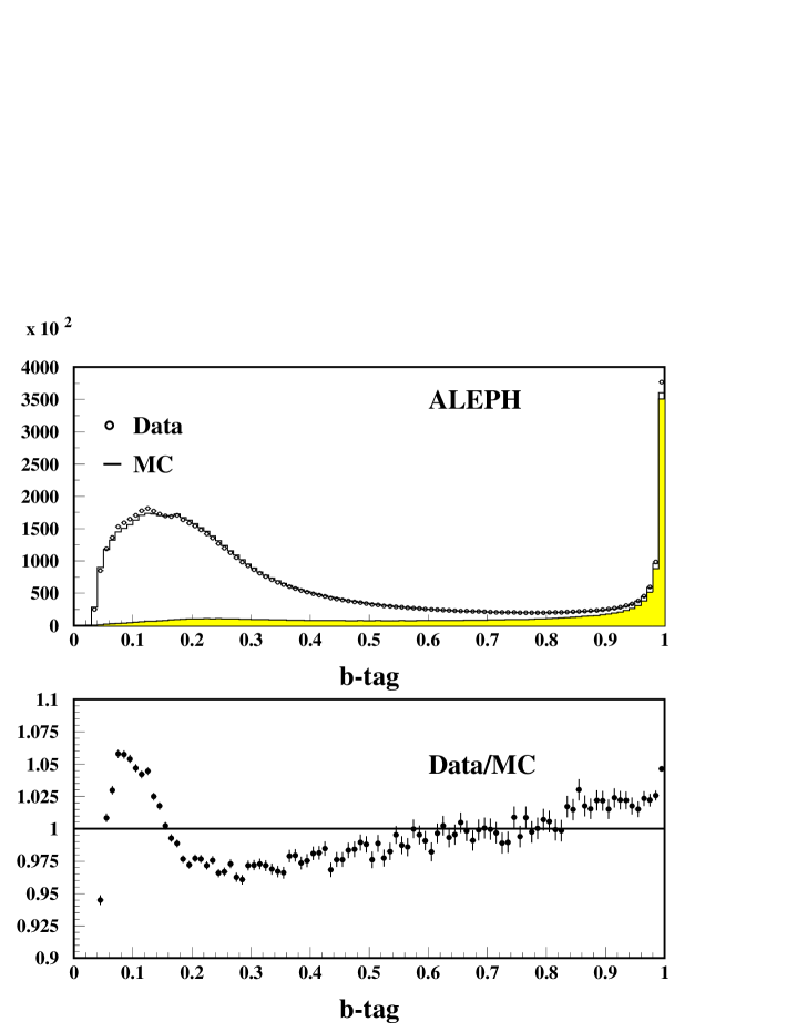
Figure 1: Distribution of the neural net hemisphere $b$-tags and the ratio between data and MC. The shaded region is the distribution for $b$-hemispheres in the MC.

The jets are clustered with the JADE algorithm using a $y_{cut}$ value of 0.02, and for each jet six variables are defined: two of them are lifetime-based; a third one is based on the transverse momentum of identified leptons; the last three are based on jet-shape properties. These quantities are

1. $\mathrm{P}_{\mathrm{jet}}$: probability of the jet being a light quark ($uds$) jet based upon impact parameters of tracks in the jet [14].

2. $\Delta\chi^{2}_{\mathrm{svx}}$: the vertex $\chi^{2}$ difference between assigning tracks in the jet both to the secondary and primary vertices compared to assigning all tracks to the primary vertex. This is based upon a secondary vertex pattern recognition algorithm which searches for displaced vertices via a three-dimensional grid point search [15];

3. $p_{\mathrm{T}}$ of identified leptons [16] with respect to the jet axis;

4. $\mathcal{S}^{\mathrm{b}}$: the boosted sphericity of the jet defined to be the sphericity of final state charged and neutral particles in the rest frame of the jet;

5. Multiplicity/ln(E_jet): the charged and neutral particle multiplicity of the jet divided by the natural logarithm of the jet energy in GeV;

6. $\Sigma p^{2}_{\mathrm{T}}$: the sum of squared transverse momenta, $p^{2}_{\mathrm{T}}$, of each charged or neutral particle with respect to the jet axis.

Among the six input variables, the lifetime tags have the largest weight. However, the inclusion of the other variables increases the $b$-quark discriminating power, especially at the most forward angles that are not covered by the vertex detector. A hemisphere $b$-tag is defined as the maximum neural net output value among the jets in the hemisphere with energies exceeding 10 GeV.

Prior to the application of the lifetime reconstruction algorithms in the MC, the track parameters have been given additional smearing and the VDET additional hit inefficiency according to a procedure described in [17]. This is necessary in order to render the MC distributions of the lifetime tags in good agreement with data. Small discrepancies still remain and combine in the neural network to give the differences between the distributions of the $b$-tag shown in Figure 1. Deviations up to about 5% between data and simulation are seen in some $b$-tag bins and for this reason the $b$-quark purity as a function of $b$-tag is determined from the data themselves.

6 The neural net charge tag

A neural network is also used to determine hemisphere charges. This technique has been employed earlier for CP violation studies in $B^{0}/\bar{B}^{0}$ decays as described in [18]. In the present analysis information regarding lepton identification is left out from the tag.

In order to achieve high tagging performance independently of the $b$-hadron species, momentum and polar angle, several charge estimators are combined. These charge tags are complemented with other variables, which do not carry information about the $b$-hadron charge in themselves, but are correlated with the relative tagging power of the charge estimators, thereby allowing an optimal combination to be achieved in the whole phase space. The two types of input variables are described separately in Sections 6.1 and 6.2.

6.1 Charge estimators

Eight charge estimators are used to provide information on the initial charge state of $b$-quark hemispheres as inclusively as possible. These are:

1. The jet charge. This is the charge estimator used in the previous analysis [2]: the weighted sum of particle charges in a hemisphere, where the weights are the particle momenta along the thrust axis, $p_{\rm L}$, raised to the power $\kappa$. Four different values of $\kappa$ are used for inputs to the neural net: 0.0, 0.5, 1.1 and 2.2. These focus on correspondingly higher values of track momenta but are of course highly correlated. Such charge estimators work well for all species of $b$-hadrons.

2. The secondary vertex charge. Using a topological vertexing algorithm combining information from all charged tracks in the hemisphere [18], a best estimate for a secondary vertex position is obtained in each hemisphere. An estimate of the charge of this vertex is calculated as:

   $$Q_{\rm vtx}\>=\>\sum_{i={\rm tracks}}w_{i}\,q_{i}\,,$$ (7)

   where $w_{i}$, calculated by a dedicated neural net [18], is the probability that track $i$ comes from the secondary vertex and $q_{i}$ is the track charge. This estimator provides a high quality charge tag for $B^{\pm}$ hemispheres, and also helps to indicate which hemispheres are more likely to contain a neutral $B$ meson.

3. The weighted primary vertex charge. For $B^{0}$ hemispheres the secondary vertex charge carries little information, but in this case the fragmentation tracks close in phase space to the $B^{0}$ have some correlation with the primary $b$-quark charge. Therefore a charge estimator, $Q_{\rm Pvtx}$, is calculated according to :

   $$Q_{\rm Pvtx}\>=\>\sum_{i={\rm tracks}}(1-w_{i})\,p_{\rm L}^{i}\,q_{i}\,/\,\sum_{i={\rm tracks}}(1-w_{i})\,p_{\rm L}^{i}\,.$$ (8)

4. The weighted secondary vertex charge, $Q_{\rm Svtx}$, is calculated in a similar manner, replacing the weight $(1-w_{i})\,p_{\rm L}^{i}$ by $w_{i}\,\left(p_{\rm L}^{i}\right)^{0.3}$ with the aim of improving the tagging for both charged and neutral $B$-decays via leading particle effects from the secondary decay.

5. Fast kaon identification is formed by another dedicated sub-net [18] trained to identify charged kaons from $b$-hadron decays. The output for the most kaon-like particle in the hemisphere is signed by the charge of the particle and used as a charge estimator.

6.2 Control variables

The following variables are used as inputs to the neural net in order to provide it with some topological and $b$-hadron specific information:

1. $|\cos\theta|$ is included since it is correlated with the quality of the secondary vertex reconstruction and hence with the tagging power of the estimators relying on the separation between tracks from the primary and secondary vertex.

2. The reconstructed $b$-hadron momentum is included because the relative accuracy of the various charge estimators depends on the $b$-hadron momentum. An estimator of this momentum is constructed from the jet closest to the line-of-flight of the $b$-hadron. The estimator is the sum of the charged track momenta in the jet, weighted by the probability that they come from the secondary vertex, and the projections of the neutral momenta onto the line-of-flight of the $b$-hadron. The missing energy in the hemisphere is also added.

3. The reconstructed proper time of the $b$-hadron is used based on the reconstructed $b$-hadron momentum and the measured decay length. The intention here is to incorporate the increased probability of $B^{0}_{d}$ mixing at long proper times.

4. The spread of track separation weights i.e. the width of the $w_{i}$ factors distribution in a given hemisphere. This allows the net to de-weight those charge estimators which suffer from an ambiguous allocation of tracks to the primary and secondary vertices in cases of high charged multiplicities and/or poor vertexing.

Figure 2: The charge difference between forward and backward hemispheres measured in the selected event sample labelled E in Figure 3. The MC distribution corresponds to an asymmetry of $A^{b}_{\rm FB}=0.0967$.

For the asymmetry calculation, the difference between the neural net outputs of the two hemispheres is used. This is shown in Figure 2 together with the MC prediction. The charge separation is seen to be reasonably well simulated, but with a slightly larger width in data than in MC (there is also a small difference in the average value of the two distributions, but this is too small to be visible on the plot).

7 Event selection

The data set used for this analysis consists of four million hadronic $Z$ decays recorded by ALEPH during the period 1991 to 1995 in a centre-of-mass energy range of $M_{Z}\pm 3\,$GeV. Events are selected according to the standard ALEPH hadronic event selection based on charged track information [19]. This selection has an efficiency of $97.5\,\%$ and the backgrounds from $Z$ decays to $\tau^{+}\tau^{-}$ and $\gamma\gamma$ interactions are estimated to be $\sim 0.3$% each. These backgrounds are reduced to the 10^-5 level after the application of the subsequent cuts and can be safely neglected.

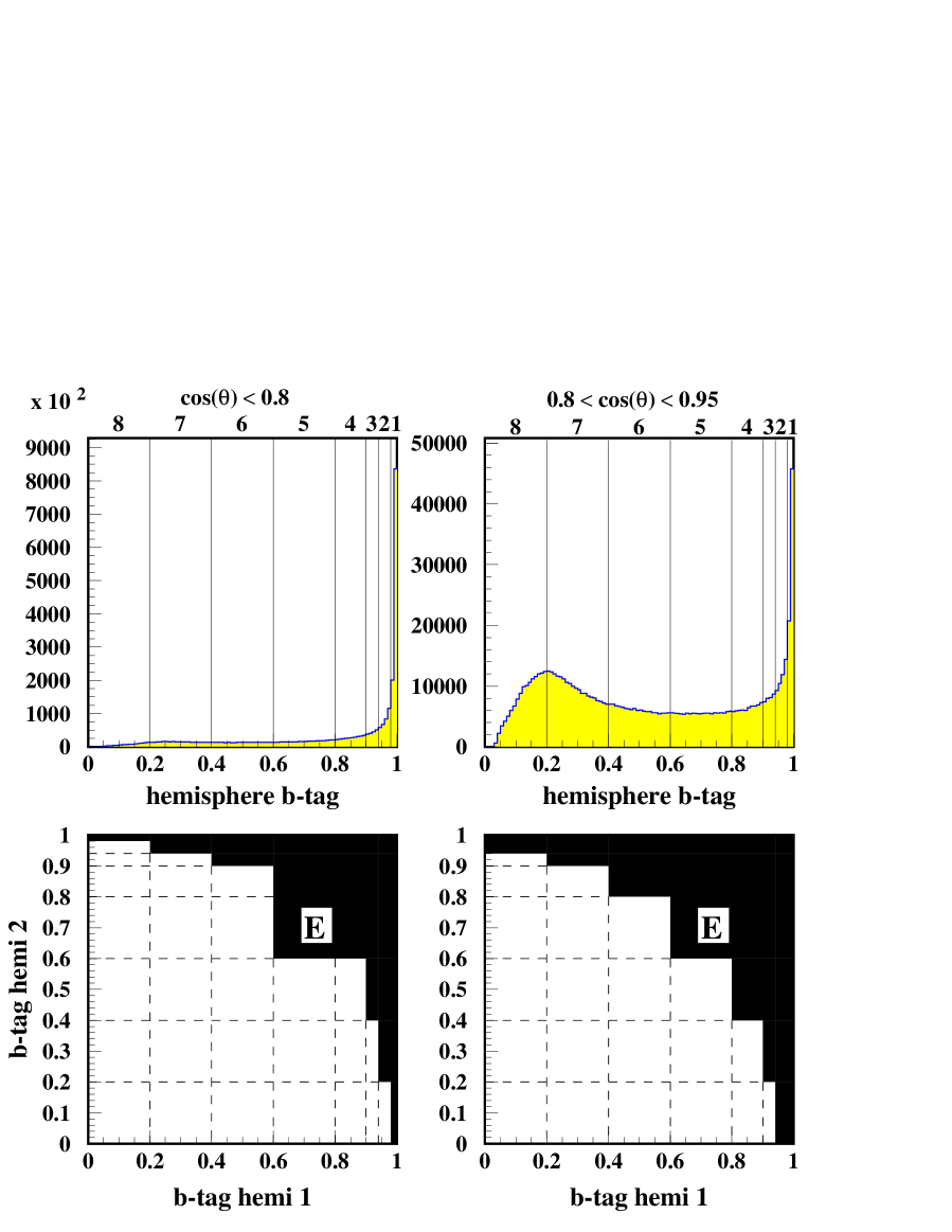
Figure 3: Upper plots: Subdivision into $b$-tag intervals with numbers above the plots enumerating the intervals. The shaded histogram is the expected $b$-tag distribution for $b$-hemispheres, shown separately for two regions of polar angle. Lower plots: The event acceptance, shown shaded and labelled E, in the plane of the two hemisphere $b$-tags.

The average beam-spot position is determined every 75 events and used to constrain the event-by-event interaction point. In order to remove lifetime information from the tracks, these are projected onto the plane perpendicular to their parent jets (unless they point behind the interaction point found in a first iteration). Combining these projections with the beam-spot position fixes the interaction point to a precision of $50\times 10\times 60\,\mu{\rm m}^{3}$ in horizontal, vertical and beam directions respectively.

The thrust axis is determined in each event from all charged tracks and calorimeter clusters using the ALEPH energy flow algorithm [7]. To ensure that a good fraction of the event is contained within the detector acceptance, the cosine of the thrust axis polar angle is required to be less than $0.95$. In order to be able to evaluate the hemisphere $b$-tag and charge tag it is required that each hemisphere has at least one charged track and at least one jet with energy greater than 10 GeV. With these selection cuts a sample of 3,734,425 hadronic $Z$ decays is retained for the remainder of the analysis.

In order to make use of double-tag methods for determining flavour purities, the $b$-tag range between zero and one is divided into eight sub-intervals as shown in Figure 3. The 672,111 events which are located in the region indicated by the black area in Figure 3, labelled E, are the ones accepted for the $A_{\mathrm{FB}}$ analysis. The acceptance is less strict in the forward region which is not covered by the vertex detector and therefore has a broader distribution of $b$-tags.

8 Determination of flavour purities

The fractions of primary quark flavours in the selected event sample are measured in the data using the double tag method, that has been used previously in e.g. the ALEPH $R_{b}$ measurement [17, 20].

In each of nine angular intervals, eight $b$-tag sub-intervals are defined as indicated in Figure 3, out of which only seven are mutually independent and the eighth is considered as “not tagged”. These give rise to 28 doubly tagged event classes and 7 singly tagged classes: $n_{ij}$ and $n_{i8}$, which are related to the tagging efficiencies by:

$$n_{ij} = \sum_{f}(2-\delta_{ij})\>\epsilon^{f}_{i}\>\epsilon^{f}_{j}\>c^{f}_{ij}\>R_{f}\>n_{{\mathrm{h}ad}}\,;\;\;\;\;\,i\leq j\,,$$

$$n_{i8} = \sum_{f}2\>\epsilon^{f}_{i}\>R_{f}(1-\sum_{j\leq 7}\epsilon^{f}_{j}\,c^{f}_{ij})\>n_{{\mathrm{h}ad}}\,;\;\;i\leq 7\,,$$ (9)

where $\epsilon^{f}_{i}$ is the probability for a primary quark of flavour $f$ to be located in interval $i$, $c^{f}_{ij}$ describes correlations between the $b$-tag values in the two hemispheres, $R_{f}$ is the $Z\rightarrow f\bar{f}$ fraction of the $Z$ hadronic decays and $n_{\mathrm{had}}$ is the total number of events in the sample under consideration. The flavour index, $f$, runs over three flavour classes only ($uds$, $c$ and $b$), hence efficiencies and correlation factors are averaged over the three light flavours.

Various assumptions are made to reduce the number of unknown parameters in Equation (9). The hemisphere correlations are taken from MC simulation and the values of $R_{f}$ are taken from previous measurements. Furthermore, it is necessary to fix the ratio of the two smallest efficiencies, where $\epsilon^{uds}_{1}\approx 0.0008$ and $\epsilon^{uds}_{2}\approx 0.0013$ according to the simulation. The ratio between these numbers is taken from simulation.

	Fitted purities			Fit$-$MC
$\cos(\theta)$	$uds$	$c$	$b$	$uds$	$c$	$b$
$0.0-0.1$	$157\pm 46\pm 3$	$1237\pm 69\pm 7$	$8606\pm 34\pm 15$	$-33$	96	$-63$
$0.1-0.2$	$239\pm 56\pm 5$	$1170\pm 77\pm 7$	$8591\pm 32\pm 14$	43	6	$-49$
$0.2-0.3$	$208\pm 48\pm 4$	$1156\pm 69\pm 7$	$8636\pm 31\pm 14$	15	13	$-28$
$0.3-0.4$	$246\pm 55\pm 5$	$1098\pm 74\pm 6$	$8657\pm 31\pm 14$	64	$-26$	$-38$
$0.4-0.5$	$200\pm 36\pm 4$	$1064\pm 56\pm 6$	$8736\pm 40\pm 14$	32	8	$-40$
$0.5-0.6$	$147\pm 42\pm 3$	$992\pm 63\pm 6$	$8863\pm 31\pm 14$	$-15$	22	$-7$
$0.6-0.7$	$197\pm 52\pm 5$	$809\pm 73\pm 5$	$8994\pm 29\pm 14$	42	14	$-56$
$0.7-0.8$	$422\pm 94\pm 16$	$366\pm 109\pm 3$	$9212\pm 30\pm 14$	238	$-242$	$-4$
$0.8-.95$	$405\pm 203\pm 5$	$883\pm 250\pm 8$	$8721\pm 57\pm 14$	27	342	$-369$

Table 2: Flavour purities of the event sample labelled E in Figure 3 as obtained from the double tag fit. The values are given in units of 10^-4. The second error is from MC statistics contributing through the assumed hemisphere tag correlations.

The remaining 20 unknown efficiencies $\epsilon^{f}_{i}$ are determined from a fit using Equations (9) leaving 15 remaining degrees of freedom in the fit.

The fitted efficiencies are combined to give event tag efficiencies by summing over the fiducial region labelled E in Figure 3:

$$\epsilon_{E}^{f}\>=\>\sum_{i,j\in E}\epsilon^{f}_{i}\,\epsilon^{f}_{j}\,c^{f}_{ij}\,,$$ (10)

and from these efficiencies the three purities are constructed as:

$${\cal P}_{E}^{f}\>=\>\frac{\epsilon_{E}^{f}R_{f}}{\epsilon_{E}^{b}R_{b}+\epsilon_{E}^{c}R_{c}+\epsilon_{E}^{uds}(1-R_{b}-R_{c})}\,,$$ (11)

where the used $R_{f}$ fractions are shown in Table 6. The result of the fit is shown in Table 2. The covariance matrix of the fitted efficiencies is propagated to the event-tag purities with diagonal elements also shown in Table 2 and correlation coefficients being typically $-90$% , +45% and $-80$% for the $uds$-$c$, the $uds$-$b$ and the $c$-$b$ purity correlations, respectively. The $\chi^{2}$ of the nine independent fits at different $\cos\theta$ averages 0.99 per degree of freedom.

Already from Figure 1 it is seen that the efficiencies in the highest $b$-tag bins are higher in the data than in the MC. The fit determines that this enhancement is slightly larger for light and charm quarks than for $b$-quarks, resulting in a $b$ purity which is about 0.5% lower than predicted by the MC in the selected sample.

9 Determination of quark charge separations

The mean values of the hemisphere charge separations, $\delta_{f}$, are determined from data in each bin of $\cos\,\theta$ using the following procedure.

The data sample is subdivided into 14 bins with flavour compositions ranging from almost pure $uds$ to almost pure $b$ flavour. The sum of squares of the two hemisphere $b$-tags is used to define the bins and the flavour compositions of these new bins are derived from the fit to the data described in the previous section.

In each bin of this event $b$-tag variable, $\bar{\delta}$ is measured according to Equation (3). A fit is performed using the 14 $\bar{\delta}$ measurements and the right side of Equation (3) with the flavour specific values $\bar{\delta}_{b}$, $\bar{\delta}_{c}$ and $\bar{\delta}_{uds}$ as free parameters. Since the $b$-tags in the 14 bins bias the charge estimator differently, additional assumptions taken from MC are needed in order to compare the 14 $\bar{\delta}$ measurements. For each flavour, the differences between the $\bar{\delta}$ in a given bin and the $\bar{\delta}$ in the E-region, $\beta=\bar{\delta}_{\mathrm{E}}-\bar{\delta}_{\mathrm{bin}}$, are held fixed at their MC values. Thus, for each flavour, the fit shifts $\bar{\delta}$ by a fixed amount in all bins, minimising the following $\chi^{2}$:

$$\chi^{2} = \sum_{i=1}^{14}\frac{\left(\bar{\delta}^{2}_{{\rm meas},i}-\sum_{f=1}^{3}{\cal P}^{f}_{i}\left(\bar{\delta}_{f}\,r_{f}-\beta^{f}_{i}\right)^{2}\right)^{2}}{\left(\Delta\bar{\delta}^{2}_{{\rm meas},i}\right)^{2}}\,,$$ (12)

where $i$ labels the $b$-tag bins and $f$ the flavours ($b$, $c$ and $uds$). The $\bar{\delta}_{f}$ appearing in the $\chi^{2}$ refers to MC events in the E-region and the correction factors $r_{f}$ are the three free parameters of the fit.

The inputs to the fit, averaged over all $\cos\theta$, are shown in Table 3 for $b$- and $c$-quarks together with the flavour combined output and the MC prediction. The fit reproduces accurately the $b$-tag dependence of $\bar{\delta}$. The angular dependence of the fitted parameters is shown in Figure 4 and, since the ratios between fitted and predicted values are consistent with being constant over angles, their average values are quoted below:

$$r_{b}=0.995\pm 0.004\,,$$

$$r_{c}=1.031\pm 0.011\,,$$

$$r_{uds}=1.009\pm 0.009\,.$$

${\cal P}_{c}$	${\cal P}_{b}$	$\beta_{c}$	$\beta_{b}$	Observed	Expected	Fitted
				$\bar{\delta}$	$\bar{\delta}$	$\bar{\delta}$
5.2	0.3	0.0676	0.1650	$0.4413\pm 0.0061$	0.4407	0.4430
8.6	0.8	0.0808	0.1559	$0.3877\pm 0.0039$	0.3851	0.3878
11.8	1.6	0.1016	0.1663	$0.3347\pm 0.0036$	0.3341	0.3371
15.5	3.0	0.1119	0.1493	$0.3115\pm 0.0035$	0.3083	0.3124
20.0	5.0	0.0979	0.1496	$0.3039\pm 0.0033$	0.3003	0.3042
24.9	8.2	0.0884	0.1284	$0.3030\pm 0.0031$	0.2960	0.3001
29.7	12.2	0.0729	0.1186	$0.3048\pm 0.0030$	0.2982	0.3029
34.4	18.4	0.0572	0.1118	$0.3011\pm 0.0028$	0.2994	0.3026
38.4	27.7	0.0465	0.0945	$0.3080\pm 0.0026$	0.3028	0.3072
36.2	45.3	0.0237	0.0813	$0.3144\pm 0.0023$	0.3092	0.3130
17.4	77.7	0.0098	0.0445	$0.3113\pm 0.0021$	0.3146	0.3157
12.5	85.8	$-$0.0104	0.0290	$0.3276\pm 0.0028$	0.3272	0.3275
7.0	92.5	$-$0.0252	0.0091	$0.3411\pm 0.0029$	0.3421	0.3420
1.2	98.8	$-$0.0802	$-$0.0455	$0.3910\pm 0.0019$	0.3941	0.3886

Table 3: From left to right: bin-by-bin flavour purities (${\cal P}$ in percent), biases ($\beta=\bar{\delta}_{\mathrm{E}}-\bar{\delta}_{\mathrm{bin}}$), measured, MC expected and fitted values of $\bar{\delta}_{\mathrm{bin}}$. The numbers in this table are integrated over all polar angles.

Figure 4: The fitted values of $\bar{\delta}_{b}$ and $\bar{\delta}_{c}$ as a function of polar angle together with the values predicted by the MC.

The average correlation coefficients of the error matrix are $-$64% between $uds$ and $c$, 25% between $uds$ and $b$ and $-$49% between $c$ and $b$. The average $\chi^{2}$ probability is 0.72 over the independent fits in nine bins of polar angle.

The fitted values of $\bar{\delta}_{f}$ are translated into the charge separations, $\delta_{f}$ by Equation (2), where the charge correlation correction factors, $(1+k_{f})$, are taken from MC. These factors vary with polar angle, averaging 1.086 for $c$-quarks and 1.092 for $b$-quarks.

In the fit of $A_{\mathrm{F}B}^{b}$ from Equation (6), the values for the charge separations, $\delta_{f}(\theta)$, are thus the MC values corrected by the $r_{f}(\theta)$ factors. The ratios between individual light quark charge separations are taken from MC. In summary, the following values are used (averaging over polar angle and showing only the diagonal elements of the statistical error matrix):

$$\delta_{b} \>=\> -0.3143\pm 0.0014\,,$$

$$\delta_{c} \>=\> +0.3733\pm 0.0039\,,$$

$$\delta_{s} \>=\> -0.1929\pm 0.0016\,,$$

$$\delta_{d} \>=\> -0.1547\pm 0.0013\,,$$

$$\delta_{u} \>=\> +0.2598\pm 0.0022\,.$$

This charge separation corresponds to an average event mis-tag of 25.6% for $b\bar{b}$ events. The result of the asymmetry fit to the peak data is

$$A^{b}_{\mathrm{FB}}(\sqrt{s}=91.232~{}{\rm GeV})\>=\>0.0997\pm 0.0027(stat).$$

10 Systematic errors

The determinations of the sample purity, the charge separation and the forward–backward asymmetry itself all rely to some extent on samples of Monte Carlo events. The features of the simulation most relevant for the analysis have been identified and varied within their errors in order to estimate the systematic uncertainty of the measurement as described in detail in the following sections.

10.1 The uds purity at large $b$-tags

In the fit yielding the flavour purities of the selected event sample it was assumed that ratio of the tiny efficiencies for selecting a light flavour with $b$-tag $>0.98$ and for selecting a light flavour with $0.94<b$-tag $<0.98$ was correctly predicted by the MC to be 0.62, averaged over polar angle. A systematic uncertainty on this ratio of $\pm 30$% is estimated by varying the track parameter smearing and the gluon splitting rates to heavy flavours in the MC. Propagating this uncertainty to the asymmetry yields a variation of $\pm 0.00037$.

10.2 Correlations between hemisphere $b$-tags

The correlation factors ($c^{f}_{ij}$ in Equation (9)) are taken from Monte Carlo simulation. The influence of the correlations on the purities, via the fitted flavour efficiencies, is limited by Equation (11) because the $b$-quark purity is high, 88% on the average. The correlation coefficient with the largest impact on the $b$ purity is the negative correlation for observing both hemispheres in the highest $b$-tag bin: $c^{b}_{11}-1=-0.02$ in the central region of the detector. It is due to the pull on the shared reconstructed primary vertex exerted by a secondary vertex from $b$-hadron decay. If that coefficient is changed by an amount $\pm 0.01$, the $b$ purity changes by the amount $\pm 2.3\cdot 10^{-4}$ in the central region. The other coefficients carry impacts on the flavour purities of size $10^{-4}$ or less for a one percent change in the coefficient.

In order to estimate the uncertainty in the correlation coefficients, the input parameters to the MC given in Table 1 are changed, one by one by the re-weighting technique, to the one $\sigma$ higher values. Two additional re-weighted MC samples are studied in order to cover effects of QCD gluon radiation and of fragmentation. In one sample the angles separating the two selected $b$-jets are forced to agree with data and in another sample the charged multiplicity of the primary vertex is forced to agree with data. The largest effects on the $b$ purities arise from changing the $x_{b}$ beam energy fraction, the charge particle multiplicities and the inter-jet angles, ranging from typically $\pm 10^{-5}$ in the central region to $\pm 10^{-4}$ at the most forward angles. The individual changes are added in quadrature to produce the total variation in the asymmetry of 0.00001.

There could be effects other than $b$-physics parameters causing an inaccurate simulation of the correlation factors. The possibilities include inaccuracies in the simulation of vertexing and of QCD effects. Therefore, a study of additional systematic errors is carried out along the lines of the ALEPH $R_{b}$ measurement [17, 20]. Here, the contribution to the correlation from a given variable $v$ is calculated as:

$$c_{ij}(v)=\frac{\int(f_{i}(v)*g_{j}(v)+g_{i}(v)*f_{j}(v))dv}{2\ (\int f_{i}(v)dv)\ (\int f_{j}(v)dv)}$$ (13)

where $f_{i}(v)$ is the fraction of hemispheres, among all hemispheres with the variable situated between $v$ and $v+dv$, having the tag $i$. Similarly $g_{i}(v)$ is the corresponding fraction with the opposite hemisphere tagged by tag $i$. The chosen variables, $v$, are the thrust polar and azimuthal angles, an estimator of the $b$-hadron momentum and the six input variables to the $b$-tagging neural network. Since the most important correlations are those involving $b\bar{b}$ events, the ten most significant of those are studied. In order to avoid having to subtract a very large non-$b$ background in some bins, a soft $b$-tag is placed before evaluating the integrals. This soft $b$-tag leaves a 64% pure $b$-sample.

For the azimuthal angle, where no significant correlation is expected, the result of Equation (13) is indeed unity within a precision of $10^{-3}$. The rest of the variables do produce correlations, but the differences between data and MC are all between $10^{-3}$ and $10^{-2}$ and hence their contribution to the error on the measured asymmetry (via the flavour purities) is again very small, in total 0.00001.

Until now only correlations in $b\bar{b}$ events have been studied. Although the individual correlations for the lighter quarks have very little impact, the possibility of a combined effect of a large number of correlations has been investigated by simply ignoring all of them in the fit (except at the very most forward angle where geometrical effects are important). This results in a change in $A^{b}_{\mathrm{FB}}$ of +0.00002. A summary of all errors connected with the estimation of flavour purities is given in Table 4.

Statistical error in the purity determination	$\pm 0.00039$
Light quark $b$-tag efficiencies	$\pm 0.00037$
Hemisphere $b$-tag correlations	$\pm 0.00003$
Total systematic error due to purities	$\pm 0.00054$

Table 4: Summary of systematic errors on the $A^{b}_{\rm FB}$ measurement from the determination of flavour purities.

10.3 Systematic uncertainties on charge separations

Various assumptions contribute to systematic uncertainties on the determination of the charge separations, $\delta_{f}$. In a first step, $\bar{\delta}_{b}$, $\bar{\delta}_{c}$ and $\bar{\delta}_{uds}$ are extracted from a fit to data, where the assumed flavour purities and charge bias corrections in the different $b$-tag bins contribute to the systematic error together with the statistical errors of the fit. In a second step, the constant of proportionality, $(1+k_{f})$, between $\bar{\delta}_{f}$ and $\delta_{f}$ contributes to the uncertainty. These systematic uncertainties are summarised in Table 5 and discussed in detail in the following.

• Flavour purities -  This is evaluated by using the purities predicted by the MC instead of the fitted purities. The full changes in the fitted values of $\bar{\delta}_{f}$ are propagated to the error on the asymmetry.

• Corrections for $b$-tag bias -  Two overlapping procedures are used to estimate this uncertainty:

  1. Each of the $b$-physics parameters listed in Table 1 are increased one at the time by one standard deviation, using re-weighted versions of the MC, and the differences in the fitted $\delta_{b}$ and $\delta_{c}$ are propagated to the asymmetry and entered as systematic errors in Table 5 . These estimates include the effect of the parameters on the charge correlation corrections discussed below. As in the case of hemisphere tag correlations, the effect of re-weighting the MC to agree with the observed primary vertex multiplicity and the observed distribution of inter-jet angles are also included. Finally, the $Vector/(Vector+Pseudoscalar)$ ratio in $D$-meson production is varied within its experimental error of 0.05 [21].

  2. The values of $\bar{\delta}_{c}$ and $\bar{\delta}_{uds}$ are fixed at their MC values instead of being left free in the fit. In this case Equation (3) can be solved directly for $\bar{\delta}_{b}$ in the E-region without any assumptions concerning bias corrections. The full difference between the result of this and the default result is taken as an independent contribution to the systematic error. This corresponds to an excursion in the fitted value of $\bar{\delta}_{c}$ by almost two times the other uncertainties on this quantity.

• Charge correlation corrections -  One contribution to the systematic error from the $(1+k_{f})$ factors is found by varying the input parameters of the MC as described above.

  Another contribution is estimated, like in the case of hemisphere $b$-tag correlations, from the difference between data and MC when building on the E-sample a “projection” of the hemisphere charge correlations along a series of observables, as follows:

  $$(1+k_{v})^{2}=\frac{\int\left(Q_{\rm same}^{+}(v)*Q_{\rm opp}^{-}(v)+Q_{\rm same}^{-}(v)*Q_{\rm opp}^{+}(v)\right)P(v)dv}{2\langle Q^{+}\rangle\langle Q^{-}\rangle}\,,$$ (14)

  where $Q^{\pm}(v)$ is the average positive or negative hemisphere charge, given the variable $v$ in either the same or the opposite hemisphere, and $P(v)$ is the probability density of $v$. Eight variables are chosen that are weakly correlated while covering the variables relevant for the charge determination. These are the thrust, the thrust axis direction, some inputs to the charge tagging neural net, the $b$-tag and the $b$-hadron momentum. The differences in $(1+k_{v})$ between data and MC are propagated to Table 5.

  This procedure relates to the simulation of charge correlations for events in the selected sample consisting mostly of $b\bar{b}$ events. Previous studies using the jet-charge technique [5, 3] have assessed the uncertainty in $k_{c}$ separately. Using a weighting power of $\kappa=0.5$ the value $k_{c}=0.085\pm 0.022$ was found, where the error includes systematic uncertainties. This value is equal to the charm charge correlation in the present study and its error is propagated as an additional contribution to Table 5.

• Light quark charge separations -  The light quark charge separations, $\delta_{u}$, $\delta_{d}$ and $\delta_{s}$, are taken from Monte Carlo, but corrected by the overall correction factor from the fit. Systematic uncertainties are ascribed according to the results of [5] which represent relative uncertainties of 2.1%, 4.0% and 1.5% for $u$, $d$ and $s$ respectively. These errors are much larger than the error on the combined light quark $\bar{\delta}_{uds}$ from the fit. However, when propagated through to $A_{\rm FB}^{b}$, the systematic uncertainties arising from light quark charges are small, in total 0.00003.

• Track parameter smearing -  The extra smearing and hit inefficiency mentioned in Section 5 also affects the charge tag. The effect of dropping these corrections to the MC altogether results in a change in the asymmetry of +0.00016 which is taken as an additional contribution to the systematic error.

Source of systematic uncertainty	$\Delta A_{\rm FB}^{b}$
Statistics in the $\bar{\delta}_{f}$ determination	0.00074
flavour purities	0.00015
$<x_{b}>$ beam energy fraction	0.00007
$<x_{c}>$ beam energy fraction	0.00000
$n_{ch}$ in $b$-hadron decay	0.00003
$B_{s}$ fraction	0.00004
$\Lambda_{b}$ fraction	0.00004
$B^{+}$ lifetime	0.00003
$B^{0}$ lifetime	0.00002
$B_{s}$ lifetime	0.00002
$b$-baryon lifetime	0.00003
$g\rightarrow{b}\bar{b}$ rate	0.00008
$g\rightarrow{c}\bar{c}$ rate	0.00004
primary multiplicity	0.00001
inter-jet angles	0.00004
$\frac{V}{V+P}$ for charm	0.00019
fixed $\delta_{c}$ and $\delta_{uds}$	0.00037
charge correlations due to thrust	0.00001
charge correlations due to $\cos\theta$	0.00008
charge correlations due to $\phi$	0.00007
charge correlations due to $b$-hadron momentum	0.00002
charge correlations due to $b$-tag	0.00000
charge correlations due to jet-charge	0.00012
charge correlations due to primary vertex charge	0.00010
charge correlations due to secondary vertex charge	0.00011
charge correlations due to kaon charge	0.00000
charm quark charge correlations	0.00016
light quark charge separations	0.00003
track parameter smearing	0.00016
Total systematic error due to charge separations	0.00093

Table 5: Summary of systematic error contributions to the $A^{b}_{\rm FB}$ measurement from the determination of charge separations.

10.4 Experimental systematic errors on $Q_{\mathrm{FB}}$

For the measuring apparatus itself to produce a fake $Q_{\mathrm{FB}}$, a forward-backward asymmetric bias in the charge measurement is needed. Such an effect could come from an asymmetry in the detector material, since nuclear interactions of the produced particles with this material give rise to an excess of charge which is measured by the total charge, $Q_{\rm tot}$, in data [5]. The asymmetry of the material is estimated by measuring the forward-backward asymmetry of photons that have converted to $e^{+}e^{-}$ pairs in the detector. This asymmetry is multiplied by the material charge component at each angle and subtracted from $Q_{\mathrm{FB}}$, causing a shift in $A^{b}_{\mathrm{FB}}$ by $0.00016\pm 0.00032$ which is taken as a contribution to the systematic error.

Another possible source of error is the modelling of the magnetic field in the extreme forward region. This is known to cause a slight difference in the momenta measured for positive and negative particles at momenta close to the beam energy and a correction, which is not quite forward-backward symmetric, is applied as default on the data to take out this effect. However, the effect on $A^{b}_{\mathrm{FB}}$ from dropping the correction is very small ($0.00002$) and this is added to the error.

10.5 Electroweak observables

Assumptions regarding electroweak observables other than $A^{b}_{\mathrm{FB}}$, e.g. $R_{b}$ and $A^{c}_{\mathrm{FB}}$, belong to a special class, since they are important for the Standard Model interpretation of the result. Their values used in this analysis are taken from the Standard Model and are listed in Table 6 together with their impacts on the measured value of $A^{b}_{\mathrm{FB}}$. In case of the branching fractions $R_{f}$, the variation in one flavour is compensated by changes in the light quark $R_{f}$’s ($f=uds$) according to their relative magnitudes.

Parameter P	$\sqrt{s}=89.416$ GeV	$\sqrt{s}=91.232$ GeV	$\sqrt{s}=92.945$ GeV	$\partial A^{b}_{\rm FB}/\partial$ P
$R_{u}$		0.17211		$-$
$R_{d}$		0.22025		$-$
$R_{s}$		0.22025		$-$
$R_{c}$		0.17154		$+0.018$
$R_{b}$		0.21585		$-0.440$
$A^{u}_{\rm FB}$	$-0.03342$	0.06507	0.12445	$+0.006$
$A^{d}_{\rm FB}$	$0.06141$	0.09982	0.12447	$-0.001$
$A^{s}_{\rm FB}$	$0.06150$	0.09983	0.12908	$-0.001$
$A^{c}_{\rm FB}$	$-0.03350$	0.06513	0.12451	$+0.103$

Table 6: Summary of Standard Model inputs used in the measurement and their influence on the measured $A^{b}_{\rm FB}$.

10.6 QCD correction

The radiation of gluons from the original quark pair can in principle lower the asymmetry. The effect is expected to be small with the present method, where the thrust-defined hemisphere charges are calibrated back to the charges of the primary quarks in these hemispheres using partly data and partly MC. However, this built-in correction may not be sufficient, since the hemispheres defined by the $q\bar{q}$ axis are not identical to those defined by the thrust. Therefore the asymmetry measured by repeating the analysis on the high statistics $b\bar{b}$ MC is compared with the generator level asymmetry in the same selected sample of MC events. The generator level asymmetry is found to be higher by a factor $1.0027\pm 0.0009$.

The most accurate calculation available of the full QCD correction in an unbiased sample of $b\bar{b}$ events results in a correction factor $1+C_{\rm QCD}=1.0354\pm 0.0063$ [22, 23]. The ratio of $C_{\rm QCD}$ to the same quantity calculated with the ALEPH MC is used to scale the residual QCD correction. Hereby the residual correction factor becomes $1.0034\pm 0.0019$, where the error takes into account the statistical uncertainty and the fraction of the theoretical error which affects this analysis.

Flavour purities	$\pm 0.00054$
Charge separations	$\pm 0.00093$
Detector asymmetries	$\pm 0.00016$
QCD correction	$\pm 0.00019$
Total systematic error	$\pm 0.00110$

Table 7: Summary of systematic errors on the $A^{b}_{\rm FB}$ measurement.

A summary of all the systematic errors is given in Table 7.

11 Cross-checks

11.1 Simultaneous fit to $R_{b}$

The selection efficiency fit which yields the flavour purities of the selected event sample has been checked by performing the fit on MC and verifying that the input efficiencies are indeed returned exactly. It has furthermore been checked that the distribution of $b$-tags in the MC agrees with that measured in the data after re-weighting the MC by the ratio of fitted to simulated flavour efficiencies.

Finally, the overall $b\bar{b}$ fraction, $R_{b}$, is left free in the fit. In order to get a stable fit, it is necessary to tie down some of the previously free parameters, and therefore the small $b$-hemisphere efficiencies for $b$-tags less than 0.6 are taken from MC in this case. The result (for the three million preselected hadronic $Z$ decays at peak energy) is $R_{b}=0.2174\pm 0.0008(stat)$. This measured value is consistent with the world average ($0.21643\pm 0.00073$ [23]). The change in the asymmetry from letting $R_{b}$ float in the fit is $-0.0005$, in agreement with the sensitivity shown in Table 6 and consistent with the uncertainty of the fit.

11.2 Lepton tagged events

Figure 5: The difference between the two hemisphere charges, signed by the lepton charge, for events in the E sample containing a high-$p_{T}$ lepton.

For the $\bar{\delta}$ fit, it has also been checked that it returns the input $\bar{\delta}_{f}$’s when applied to the MC.

The sample of events with an identified high–$p_{T}$ lepton offers an additional check on the assumptions entering the $b$-charge tag. This check is, however, limited by uncertainties in the lepton tagging due to $c\rightarrow l$, $b\rightarrow c\rightarrow l$ and $B^{0}\rightarrow\bar{B}^{0}$ transitions as well as lepton mis-identification. These uncertainties are reduced to below the $10^{-2}$ level by placing a high–$p_{T}$ cut of 1.5 GeV/$c$ on the lepton sample. The distribution of the signed difference between the two hemisphere charges in such events is shown in Figure 5. The sign of the lepton provides the $b\bar{b}$ orientation in the event and allows a measurement of $\delta_{b}=-0.3395\pm 0.0016$, after subtracting the 3.8% non-$b$ background in this sample. This is a factor $0.990\pm 0.006$ smaller than the same quantity measured in the $q\bar{q}$ MC. The corresponding ratio between the $\bar{\delta}_{b}$’s was found to be $0.995\pm 0.004$ in Section 9. This then provides a check on the MC prediction of $k_{b}$:

$$\frac{(1+k_{b})}{(1+k_{b})^{\mathrm{MC}}}=\frac{\delta_{b}}{\delta_{b}^{\mathrm{MC}}}/\frac{\bar{\delta}_{b}}{\bar{\delta}_{b}^{\mathrm{MC}}}=0.995\pm 0.007\,(stat)\,.$$

11.3 Stability checks

In order to study the stability of the analysis the accepted region in the plane of the two $b$-tags is varied over a wide range. The results for peak data shown in Table 8 are consistent within statistical errors.

events selected	$b$ purity	raw $A^{b}_{\rm FB}$	purity corrected	charge corrected
380086	0.967	0.0999	0.1006	0.1002 $\pm$ 0.0031
491011	0.938	0.0987	0.0996	0.0994 $\pm$ 0.0028
596618	0.886	0.0990	0.0999	0.0997 $\pm$ 0.0027
643773	0.853	0.0995	0.1006	0.1007 $\pm$ 0.0027
797132	0.749	0.1001	0.1006	0.1007 $\pm$ 0.0027

Table 8: Results on peak data for various event selections characterised by the sizes of the samples and their (predicted) $b$ purities. The event selection shown in bold-face is the chosen one, the E-sample.

The measurements performed for each LEP I year in the data recorded at $Z$ peak energies are shown in Table 9. They are seen to be consistent with being constant.

year	$A^{b}_{\rm FB}$
1991	0.0884 $\pm$ 0.0125
1992	0.0992 $\pm$ 0.0063
1993	0.1079 $\pm$ 0.0075
1994	0.0997 $\pm$ 0.0040
1995	0.0966 $\pm$ 0.0072
average	0.0997 $\pm$ 0.0027

Table 9: Results on peak data for each LEP I year.

12 Results and conclusions

The fit to Equation (6) is performed in three intervals of collision energy, $\sqrt{s}$, with the results shown in Figure 6. The asymmetries are then multiplied by the QCD correction factor of $1.0034$ giving, for the sample of events recorded closest to the $Z$ peak, the value:

$$A^{b}_{\mathrm{FB}}(\sqrt{s}=91.232~{}{\rm GeV})=0.1000\pm 0.0027(stat)\pm 0.0011(syst)\,.$$

The corresponding values averaged over two off–peak energy ranges are

$$A^{b}_{\mathrm{FB}}(\sqrt{s}=89.472~{}{\rm GeV})=0.0436\pm 0.0119(stat)\,,$$

$$\vspace{0.3cm}A^{b}_{\mathrm{FB}}(\sqrt{s}=92.950~{}{\rm GeV})=0.1172\pm 0.0097(stat)\,.$$

The variation of $A^{b}_{\mathrm{FB}}$ with centre-of-mass energy is shown in Figure 7 and compared with the Standard Model prediction. The three values are extrapolated to $M_{Z}=91.1874$ GeV using ZFITTER [24], giving the combined value:

$$A^{b}_{\mathrm{FB}}(\sqrt{s}=M_{Z}) = 0.0977\,\pm\,0.0025(stat)\,\pm\,0.0011(syst)$$

$$+0.103\,(A^{c}_{\mathrm{FB}}-0.06513)-0.440(R_{b}-0.21585)\,.$$

Figure 6: The forward-backward $b\bar{b}$ asymmetry as a function of thrust polar angle at three center-of-mass energies. The errors shown are statistical only.

Figure 7: The $\sqrt{s}$ dependence of $A^{b}_{\mathrm{FB}}$. The errors shown are the statistical errors and the curve is the ZFITTER prediction, adjusted to reproduce the average fitted asymmetry at $\sqrt{s}=M_{Z}$.

In order to interpret the result in terms of the Standard Model, a QED and $Z-\gamma$ interference correction of 0.0038 is applied according to [23] to give the pole asymmetry, $A^{0,b}_{\rm FB}$, which is then iterated using BHM [25] until consistent values for $A^{0,b}_{\rm FB}$, $A^{c}_{\rm FB}$ and $R_{b}$ are reached. The result is

$$A^{0,b}_{\rm FB} = 0.1009\,\pm\,0.0027\,\pm\,0.0012$$

using $A^{c}_{\rm FB}=0.0623$ and $R_{b}=0.21653$. The errors have been obtained from iterating the value one standard deviation above the measured $A^{b}_{\rm FB}$. The corresponding weak mixing angle is

$${\rm sin^{2}}\theta_{\rm W}^{\rm eff}=0.23193\pm 0.00056\,.$$

This is to date the best $A^{b}_{\rm FB}$ measurement [2,26-34] and provides the single most precise measurement of ${\rm sin^{2}}\theta_{\rm W}^{\rm eff}$ at LEP. The value is in agreement with the present world average value [23].

References

-
[1]
S. Glashow, Nucl. Phys. 20 (1961) 579; A. Salam, in
Elementary Particle Theory, ed. N. Svartholm, (1968).
S. Weinberg, Phys. Rev. Lett. 19 (1967) 1264. - [2] ALEPH Collaboration, “Determination of A using jet charge measurements in Z decays”, Phys. Lett. B426 (1998) 217.
- [3] ALEPH Collaboration, “Measurement of A in Lifetime-Tagged Heavy Flavour Decays”, Phys. Lett. B335 (1994) 99.
- [4] ALEPH Collaboration, “Measurement of Charge Asymmetry in Hadronic Z Decays”, Phys. Lett. B259 (1991) 377.
- [5] ALEPH Collaboration, “Determination of using jet charge measurements in hadronic Z decays”, Z. Phys. C71 (1996) 357.
- [6] ALEPH Collaboration, “A Detector for Electron-Positron Annihilations at LEP”, Nucl. Instr. Meth. A294 (1990) 121.
- [7] ALEPH Collaboration, “Performance of the ALEPH detector at LEP”, Nucl. Instr. Meth. A360 (1995) 481.
- [8] T. Sjöstrand, Comp. Phys. Comm. 82 (1994) 74.
- [9] ALEPH Collaboration, “Studies of Quantum Chromodynamics with the ALEPH detector”, Phys. Rep. 294 (1998) 1.
- [10] ALEPH, CDF, DELPHI, L3, OPAL and SLD, “Combined results on b-hadron production rates, lifetimes, oscillations and semileptonic decays”, CERN EP/2000-096, submitted to 1999 summer conferences.
- [11] The LEP heavy flavour working group, “Input parameters for the LEP/SLD electroweak heavy flavour results for summer 1998 conferences”, www.cern.ch/LEPEWWG/heavy/lephf9801.ps.gz.
- [12] C. Peterson et al., Phys. Rev. D27 (1983) 105.
- [13] ALEPH Collaboration, “Searches for the Neutral Higgs Bosons of the MSSM in collisions at centre-of-mass energies of 181-184 GeV”, Phys. Lett. B440 (1998) 419.
- [14] ALEPH Collaboration, “A precise measurement of ”, Phys. Lett. B313 (1993) 535.
- [15] ALEPH Collaboration, “An investigation of and oscillations”, Phys. Lett. B322 (1994) 441.
- [16] ALEPH Collaboration, “Heavy quark tagging with leptons in the ALEPH detector”, Nucl. Instr. Meth. A346 (1994) 461.
- [17] ALEPH Collaboration, “A measurement of Rb using a lifetime-mass tag”, Phys. Lett. B401 (1997) 150.
- [18] ALEPH Collaboration, “Study of the CP asymmetry in decays in ALEPH”, Phys. Lett. B492 (2000) 259.
- [19] ALEPH Collaboration, “Measurement of the Z resonance parameters at LEP”, Eur. Phys. J. C14 (2000) 1.
- [20] ALEPH Collaboration, “A measurement of Rb using mutually exclusive tags”, Phys. Lett. B401 (1997) 163.
- [21] ALEPH Collaboration, “Study of charm production in Z decays”, Eur. Phys. J. C16 (2000) 597.
- [22] D. Abbaneo et al., “QCD corrections to the forward-backward asymmetries of c and b quarks at the Z pole”, Eur. Phys. J. C4 (1998) 185.
- [23] The LEP and SLD Experiments, “A combination of preliminary electroweak measurements and constraints on the Standard Model”, CERN EP/2001-021, February 2001.
- [24] D. Bardin et al., CERN-TH 6443-92 (May 1992).
- [25] W. Hollik et al., Forschr. Phys. 38 (1990) 3, 165.
- [26] DELPHI Collaboration “Measurement of in hadronic Z decays using a jet charge technique” Eur. Phys. J. C9 (1999) 367.
- [27] L3 Collaboration “Measurement of the and forward–backward asymmetries at the resonance” Phys. Lett. B439 (1998) 225.
- [28] OPAL Collaboration “Measurement of b quark forward backward asymmetry around the peak using jet charge and vertex charge”, Z. Phys. C75 (1997) 385.
- [29] ALEPH Collaboration “Measurement of the forward backward asymmetry and mixing using high-pT leptons”, Phys. Lett. B384 (1996) 414.
- [30] DELPHI Collaboration “Measurement of the forward–backward asymmetry of using prompt leptons”, Z. Phys. C65 (1995) 569.
- [31] L3 Collaboration “Measurement of the forward backward asymmetry and the mixing parameter using prompt leptons”, Phys. Lett. B448 (1999) 152.
- [32] OPAL Collaboration “Measurement of heavy quark forward backward asymmetries and average B mixing using leptons in multihadronic events”, Z. Phys. C70 (1996) 357.
- [33] DELPHI Collaboration “Measurement of the forward backward asymmetries of c and b quarks at the Z pole using reconstructed D mesons”, Eur. Phys. J. C10 (1999) 219.
- [34] OPAL Collaboration “A measurement of charm and bottom forward–backward asymmetries using D mesons at LEP”, Z. Phys. C73 (1996) 379.