M05 Precision Measurement of $g_{\mu}-2$ at BNL

Abstract

The Muon $(g-2)$ Experiment (E821) at Brookhaven National Laboratory (BNL) has measured the anomalous magnetic moment of the positive muon to an unprecedented precision of 1.3 parts per million. The result, $a_{\mu^{+}}=\frac{g-2}{2}=11\ 659\ 202(14)(6)\times 10^{-10}$, is based on data recorded in 1999 and is in good agreement with previous measurements. Upcoming analysis of data recorded in 2000 and 2001 will substantially reduce the uncertainty on this measurement. Comparison of the new world average experimental value with the most comprehensive Standard Model calculation, $a_{\mu}(SM)=11\ 659\ 159.6(6.7)\times 10^{-10}$, yields a difference of $a_{\mu}({\rm exp})-a_{\mu}({\rm SM})=43(16)\times 10^{-10}$.

1 Introduction

Lepton anomalous magnetic moments arise from purely quantum mechanical effects, predominantly through higher order corrections to the $ll\gamma$ vertex. Precision measurements of these quantities have played an important role in the development of quantum field theory throughout the last century and continue to test the limits of our theoretical knowledge even today. Currently, the electron anomaly is one of the most precisely measured quantities in physics, known to an extraordinary accuracy of 4 parts per billion (ppb)[1]. Even at this level, it includes contributions from QED loop corrections only. As a result, it currently provides the best determination of the fine structure constant, under the assumption of the validity of QED.

The muon anomaly, on the other hand, has now been measured to a level of 1.3 parts per million (ppm)[2], as discussed in this note. Although this measurement is about 350 times less precise than that of the electron, it is already far more sensitive to hadronic and electroweak loop contributions, as well as any new, non-Standard Model effects. This is because the strength of such virtual loop terms is generally proportional to the square of the relevant mass scale, thus giving an enhancement of $m_{\mu}^{2}/m_{e}^{2}\approx 40,000$ in the contribution to the muon relative to the electron. In essence, the higher mass scale of the muon provides a much more effective probe of short-distance phenomena.

The anomalous magnetic moment is generally written as $a=\frac{g-2}{2}$, where the $g$-factor relates the magnetic moment of the particle to its spin, $\vec{\mu}=g(e/2mc)\vec{S}$. In the SM, the contributions to the muon anomaly can be written as the sum of three general classes of diagrams:

$$a_{\mu}({\rm SM})=a_{\mu}({\rm QED})+a_{\mu}({\rm Hadronic})+a_{\mu}({\rm Weak}).$$ (1)

Table 1 gives a breakdown of these terms with their relative contributions both to the value and uncertainty of $a_{\mu}$(SM). As in the electron case, the QED term dominates; however, hadronic and even weak contributions already come into play at the ppm level. Indeed, the previous measurement of $a_{\mu}$ conducted at CERN in the 1970’s had already demonstrated the presence of the hadronic contribution with an uncertainty of 7.3 ppm[5], mostly statistical. One of the initial design goals of the BNL experiment was a factor of 20 improvement (0.35 ppm) on the CERN result, giving a more than $3\sigma$ sensitivity to the weak contribution. It is interesting to note that this measurement has now been conducted four times (three times at CERN) and each time the result has been sensitive to theoretical contributions at a new level of computation.

Table 1: Standard Model contributions to $a_{\mu}$[3, 4].

Term	Value $(\times 10^{-11})$	Rel. Cont. (ppm)
$a_{\mu}$(QED)	116 584 705.7(2.9)	$10^{6}\pm 0.02$
$a_{\mu}$(Hadronic)	6739(67)	$57.79\pm 0.57$
$a_{\mu}$(Weak)	151(4)	$1.30\pm 0.03$
$a_{\mu}$(SM)	116 591 596(67)	$\pm 0.57$

The uncertainty in the theoretical value of $a_{\mu}$ is currently dominated by knowledge of the hadronic term. Because of the non-perturbative aspects of low energy QCD, evaluation of this term is not possible from first principles and requires input from experiment, specifically $e^{+}e^{-}\rightarrow$ hadrons (and, recently, hadronic $\tau$-decay) cross-sections down to the pion production threshold. Measurement of these cross-sections is absolutely crucial to the interpretation of any $a_{\mu}$ result. Accordingly, improvement is expected soon from the experimental programs in Novosibirsk[6] and Beijing[7]. Their work is discussed elsewhere in these conference proceedings, along with goals in the longer term[8].

A recent review of the current state of the theory can be found in reference [9] and the citations therein, as well as other presentations in this conference session[10].

2 The BNL Experiment

The experimental principle in the Brookhaven experiment is similar in concept to that of the final CERN experiment[5]. A polarized muon beam is stored in a highly uniform, circular, dipole magnet and the decay rate of muons in flight is measured with high precision. In the presence of a magnetic and electric field, the muon spins precess in the lab frame with the angular frequency

$$\vec{\omega}_{a}=-\frac{e}{m_{\mu}}\left[a_{\mu}\vec{B}-\left(a_{\mu}-\frac{1}{\gamma^{2}-1}\right)\vec{\beta}\times\vec{E}\right].$$ (2)

In this expression, $\vec{\omega}_{a}$ is the angular frequency of the spin vector relative to the momentum vector. This frequency is proportional to $a_{\mu}$ itself, not $g$, enabling a higher precision direct measurement of the anomaly. The beam is focused in the ring vertically using an electrostatic quadrupole field. At a specific “magic” momentum, the second term in equation 2 drops out and the spin precession is unaffected by the focusing electric field. This momentum, $p_{\mu}=3.094$ GeV/c $(\gamma=29.3)$, sets the scale of the experiment, some parameters of which are shown in table 2.

Measurement of $a_{\mu}$ thus requires simultaneous determinations of both $\omega_{a}$ and the magnetic field. In practice, the magnetic field is determined using an NMR system that measures the free proton precession frequency in the same magnetic field seen by the muons. The anomaly is then extracted through the relation

$$a_{\mu}=\frac{\omega_{a}/\omega_{p}}{\mu_{\mu}/\mu_{p}-\omega_{a}/\omega_{p}}$$ (3)

where the only external input is the ratio of muon to proton magnetic moments, $\mu_{\mu}/\mu_{p}=3.18334539(10)$[11]. This expression enables a natural separation of the measurement into two independent analyses, one of the field and one of the muon spin precession. Any experimenter bias can be eliminated by maintaining secret offsets between the two analysis groups. Once the analyses are complete, the results are frozen, the offsets are revealed and only then is the value of $a_{\mu}$ determined.

Table 2: E821 parameters

Parameter	Value
$B_{0}$	1.45 T
Orbit Radius	7.112 m
Storage Region Diameter	9 cm
Momentum	3.09 GeV/c
$\gamma$	29.3
$\gamma\tau$	64.4 $\mu s$
Cyclotron Frequency	6.70 MHz
g-2 Frequency	0.229 MHz
Field Index (n)	0.137
Horizontal Tune $(\nu_{h})$	0.93
Vertical Tune $(\nu_{v})$	0.37
AGS storage	$6\times 10^{13}$ protons
AGS rep rate	0.38 Hz
Beam width $(\sigma)$	25 ns

2.1 The muon beam

The Alternating Gradient Synchrotron (AGS) delivers up to $6\times 10^{13}$ protons, at an energy of 24 GeV, in 12 bunches (6 in 1999) every 2.5 seconds. The bunches are extracted every 33 ms and directed onto a nickel target. Pions of $\approx 3.1$ GeV/c are transported from the target down a 116 m beamline where about 50% decay into muons. Forward-going muons are then momentum selected for injection into the muon storage ring with a polarization of $\approx 96\%$.

The muons enter the ring through a hole in the magnet yoke and pass through a field-free region supplied by a DC superconducting inflector magnet[12]. The fringe field of the inflector magnet is contained by a superconducting shield designed to limit its effect to $\sim 1$ ppm at 2 cm. Upon exiting the inflector channel, the muons are in an orbit offset by 7.7 cm from the center of the storage region. A fast, pulsed magnet provides the $\approx 11$ mrad kick needed to move the beam onto a central orbit. This kicker magnet reduces the storage ring field locally by 0.016 T for $\approx 450$ ns with less than a 0.1 ppm residual effect after 20 $\mu$s.

This direct muon injection technique is one of the major technical improvements of this experiment compared to the pion injection technique of the CERN experiment[5], allowing for more efficient injection with greatly reduced background. Approximately one muon is stored for every $10^{9}$ protons on target.

2.2 The storage ring magnet

A cross-sectional view of the storage ring magnet[13] is shown in figure 1. It is a continuous, superferric, C-shaped magnet with a radius of 7.112 m at the center of the storage region. The field is excited by superconducting coils carrying a current of 5.2 kA and is shaped by high-precision iron pole pieces. The pole pieces are 10 degrees long and separated by 75 $\mu$m Kapton-insulated gaps in order to avoid irregular eddy current effects. Vertical air gaps decouple the pole pieces from the yoke steel and allow the insertion of iron wedges which are used both to compensate for the natural quadrupole term due to the C-shaped geometry and to reduce the azimuthal field inhomogeneity. A series of edge shims are used to reduce the local field variations over the beam cross-section and current sheets glued to the pole faces reduce the variations in the integral field. Field changes due to ambient temperature fluctuations are reduced by insulating both the yoke and pole pieces. A feedback loop from the NMR system to the magnet power supply compensates for drifts in the overall dipole term. Monitoring and analysis of the magnetic field is discussed in the next section.

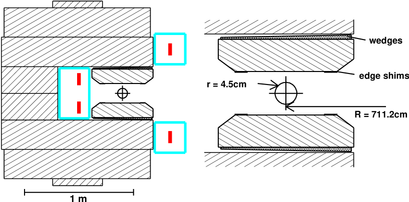
Figure 1: Cross-section of the $(g-2)$ storage ring magnet with an expanded view of the magnet gap region. The superconducting coils run perpendicular to the page in three cryostat boxes as shown. The 9 cm diameter circular beam storage region is indicated.

The electrostatic quadrupoles, which provide the vertical beam focusing, are mounted inside the beam vacuum chamber in four symmetrically placed locations. Each quadrupole consists of four plates traversing $39^{\circ}$ in azimuth and was operated at 24 kV for up to 1.4 ms. This provided a weak-focusing field index of $n\simeq 0.137$, sufficiently removed from beam and spin resonances.

The storage aperture is defined by a set of 9 cm diameter circular collimators. This circular cross-section reduces the coupling of higher order field multipoles to the beam distribution. The collimators are also used to scrape off the tails of the beam distribution during the first 15 $\mu s$ after injection, thus reducing beam losses during the measurement period. This is accomplished by lowering the voltage on the inner and bottom quadrupole plates to shift the central beam orbit by up to several millimeters.

3 Magnetic Field Analysis

The first part of the $a_{\mu}$ analysis requires a detailed measurement of the magnetic field averaged over the ensemble of stored muons. One of the major advances of the BNL experiment is the ability to map out the magnetic field in vacuo throughout the storage region. This is done using a hermetically sealed trolley containing a matrix of 17 NMR probes. The trolley moves on fixed rails inside the vacuum chamber, measuring about 6000 points in azimuth, every 7 mm. Uncertainty in the azimuthal position of the trolley contributes a 0.1 ppm systematic error to the field measurement.

Figure 2 shows the field mapped by the central trolley probe around the storage ring. In 1999, a residual fringe field in the inflector region caused a dip in the central field, visible near $350^{\circ}$, which contributed 0.2 ppm to the field systematic error. This effect is also visible in the lower right corner of figure 3, which shows a typical field profile across the storage region, averaged over azimuth. The inflector was replaced before the 2000 run, thus eliminating this effect.

Figure 2: Magnetic field measured with the central trolley probe relative to an arbitrary reference $B_{0}$ vs. azimuthal angle around the storage ring. The dip due to the inflector occurs near $350^{\circ}$.

Figure 3: Typical multipole expansion of the field as measured by the NMR trolley. The field is averaged over azimuth and one ppm contours are shown with respect to a central field value of $B_{0}=1.451\ 266$ T. The circle indicates the beam storage region and the multipole amplitudes are measured at the 4.5 cm radius.

Field mappings are conducted every 3 days on average. In the interim period, the field is tracked using about 150 NMR probes located in the upper and lower walls of the vacuum chamber. The tracking uncertainty is 0.15 ppm, as determined by comparison of the average field measured by the fixed probes to that measured by the trolley during each field mapping. Before and after data-taking periods, the trolley probes are calibrated in air against a standard spherical water probe with an accuracy of 0.2 ppm. Two largely independent field analyses were conducted using different selections of NMR probes. The results agreed to within 0.03 ppm.

The field integral encountered by the muon beam is studied by tracking 4000 muons for 100 turns through a measured field map. The simulation shows that the average field integral over the muon paths is equivalent, within 0.05 ppm, to the azimuthally averaged field measurement taken at the beam center. The radial center of the beam is known to be $3.7\pm 1$ mm outside of the central orbit based on studies of the bunched beam rotation frequency[14]. The vertical center is measured to be $2\pm 2$ mm above the central orbit using scintillating fiber beam monitors, front scintillator detectors, and the traceback chamber[15]. These measurements contribute an additional 0.12 ppm to the uncertainty in $\widetilde{\omega}_{p}$, as shown in table 3. The final value is $\widetilde{\omega}_{p}=61\ 791\ 256\pm 25$ Hz (0.4 ppm).

Table 3: Systematic errors for the $\widetilde{\omega}_{p}$ analysis

Source of errors	Size [ppm]
Calibration of trolley probes	$0.20$
Inflector fringe field	$0.20$
Interpolation with fixed probes	$0.15$
Others $\dagger$	$0.15$
Uncertainty from muon distribution	$0.12$
Trolley measurements of $B_{0}$	$0.10$
Absolute calibration of standard probe	$0.05$
Total systematic error on $\widetilde{\omega}_{p}$	$0.4\,~{}$

$\dagger$ higher multipoles, trolley temperature and its power supply voltage response, and eddy currents from the kicker.

4 Spin Precession Analysis

The spin precession frequency is obtained from the muon decay time spectrum. In the muon rest frame, the parity violating nature of the weak decay $\mu^{+}\rightarrow e^{+}\nu_{e}\bar{\nu}_{\mu}$ causes the positrons to be emitted preferentially along the muon spin direction. When boosted into the lab frame, this results in a strong correlation between the positron energy and the angle between the muon spin and momentum vectors. The decay positrons, ranging in energy from 0-3.1 GeV, spiral in towards the center of the ring where they are detected by 24 lead/scintillating fiber calorimeters[16] placed symmetrically along the inner wall of the vacuum chamber. The number of positrons observed above an energy $E_{t}$ is modulated by the muon spin precession, yielding a count rate of

$$N(t)=N_{0}(E_{t})e^{-t/\gamma\tau}[1+A(E_{t})\cos(\omega_{a}t+\phi_{a}(E_{t}))]$$ (4)

where $\gamma\tau\approx 64.4\ \mu s$ is the dilated muon lifetime. The normalization, phase and asymmetry all depend on the energy threshold. In fitting to this function, the statistical uncertainty in $\omega_{a}$ goes as $1/(\sqrt{N}A)$. In the BNL experiment, a special scalloped vacuum chamber design ensured that positrons entering the face of the calorimeter would traverse similar paths through the chamber wall. This improves the energy resolution and, therefore, the asymmetry. For an energy threshold of 2 GeV, the asymmetry is $\approx 0.4$.

The calorimeter pulses are sampled by custom-built 400 MHz waveform digitizers (WFD) which are clocked by the same LORAN-C frequency receiver used in the NMR system, thus avoiding possible systematics due to slewing time standards. Pulses above a predetermined hardware energy threshold of $\sim 900$ MeV trigger the WFD to record at least 16 8-bit ADC samples (40 ns) on both the fast-rising edge and slower tail of the pulse. Single pulses have a typical width of $\sim 5$ ns and multiple pulses can be resolved if their separation exceeds 3 to 5 ns. Pulses with energies below the hardware threshold can therefore be seen if they appear within the sampling time around a trigger pulse. This property of the WFD is useful for pileup studies as described below.

The decay spectrum from the 1999 run, containing $\sim 1$ billion measured positrons, is shown in figure 4. With this large a data sample, several effects that cause a deviation from the ideal functional form of equation 4 become statistically significant. Determination of an appropriate functional form is, therefore, an important experimental challenge. Four independent analyses were conducted with somewhat different approaches. All were forced to confront several common issues which are enumerated below.

Figure 4: Observed decay positron spectrum in 1999.

1. Pileup Effects: With the higher data rate in 1999, positron pileup in the calorimeters became a relevant issue in the analysis. Pileup events occur when two positrons arrive within the 3-5 ns deadtime interval of the pulse finding algorithm. This changes the number of counts above threshold in a rate-dependent fashion $(\propto(dN/dt)^{2})$. Thus, the effect is largest early in the fill and dies out exponentially with half the dilated muon lifetime. The effect on the count rate can be positive or negative: two pulses below threshold can overlap to mimic a single pulse above threshold, thus adding a count, or two pulses above threshold can overlap to mimic a single pulse, thus losing a count.

   Aside from affecting the count rate, the pileup pulses arrive with a different phase than $\phi_{a}$ in equation 4. Since the phase is highly correlated with $\omega_{a}$ in the fit, failure to take the pileup into account can lead to a shift in the measured frequency. The pileup functional form can be added to the fit, but the strong correlation with $\phi_{a}$ requires that the pileup phase be fixed. The pileup phase, however, is difficult to measure.

   Another approach is to correct the spectrum for pileup effects prior to fitting. This can be done by subtracting a pileup spectrum that is statistically constructed from the data itself. The technique is based on the presumption that the likelihood of a second pulse arriving within the deadtime window around the first pulse is equal to the likelihood that it will arrive within a similar time interval a few nanoseconds earlier or later. It is made possible due to the extended pulse sampling provided by the WFD, as described above.

   Two equivalent software methods are used to correct the time spectrum. One measures the effect of artificially increasing the deadtime and uses the result to extrapolate back to the zero deadtime case. The other constructs a pileup spectrum out of pulses appearing within a fixed time window on the tail of each trigger pulse, then subtracts it from the original time spectrum. Both methods can only fully correct data sets with energy thresholds of at least twice the hardware trigger threshold. This lead to a choice of $E\geq 2$ GeV in the analysis. With this energy selection, the pileup level is about 1% at the beginning of the fits.

   Pileup pulses below detectable energy thresholds are not corrected by this procedure. Since these pulses affect both the baselines and the pulse heights, they do not change the pulse energies on average. They can, however, change both the measured phase and asymmetry. The asymmetry is more sensitive to this effect, so it is used to set a limit on the shift in $\omega_{a}$.

2. AGS background: Imperfect proton extraction from the AGS sometimes leads to particles coming down the beamline and entering the storage ring during the $\sim 1$ ms data collection period. Some of these particles, mostly positrons, create background pulses in the detectors which can enter the data sample. These pulses appear with a specific time structure, defined by the 2.694 $\mu s$ AGS cyclotron period, and a specific azimuthal distribution around the ring, which can be exploited to enhance their effect and measure the level of contamination. In 1999, the relative AGS background level was $\sim 10^{-4}$ which, simulations show, leads to an uncertainty of $\pm 0.1$ ppm in $\omega_{a}$. In subsequent runs, this background level has been reduced by employing a fast sweeper magnet to close off the beamline, downstream of the target, once the main bunch has passed. Monitoring of the background level has also improved by periodically suppressing the quadrupole voltages for a fill to look for background without the presence of stored beam.

3. Muon Losses: Muon beam losses during the data collection period can distort the exponential decay form. Such losses are minimized by controlled scraping of the beam before the start of the fit, as described above. Remaining losses are taken into account by multiplying the functional form of equation 4 with an extra loss term:

   $$l(t)=1+n_{l}e^{-t/\tau_{l}}$$ (5)

   These losses are also studied using coincident signals in the front scintillation counters mounted on groups of three adjacent calorimeters.

4. Gain and Timing Shifts: Detector gain and timing stability are monitored with a pulsed laser system to strict tolerances. Drifts in gain are also observable through changes in the positron energy spectra. Timing shifts are stable to within 20 ps over the first 200 $\mu$s of the fit (0.1 ppm) while gain changes are below 0.1% for all but two of the detectors. Two of the analyses apply a gain correction, one through the use of a time-dependent energy threshold and one by incorporating the gain dependence into the fitting function.

5. Coherent Betatron Oscillations: The inflector aperture is smaller than the storage ring aperture, so the phase space for betatron oscillations, defined by the acceptance of the storage ring, is not filled. With ideal injection, this leads to a modulation of the horizontal and vertical beam widths at a characteristic frequency defined by the field index. However, because the muon kicker was forced to operate slightly below its design value, the horizontal injection kick was insufficient to place the beam onto the ideal orbit. This resulted in oscillation of the beam centroid around the central orbit at the betatron frequency. These coherent betatron oscillations (CBO) are observed directly using a set of scintillating fiber beam monitors as shown in figure 5. Note that the oscillation frequency is determined by the beam tune ($f\approx f_{c}(1-\sqrt{1-n})$, with $f_{c}$ the cyclotron frequency) and can be changed using different quadrupole settings. In the recently completed 2001 run, two different field indices were used in order to study this effect further.

   The beam oscillation is also visible in the positron time spectrum because the detector acceptance is a function of the muon decay position. Fourier analysis of the positron data yields a frequency of $\omega_{b}/2\pi=(470.2\pm 0.2\ {\rm kHz})$. This effect dies out slowly, with a time constant of $\sim 100\ \mu s$ and can be effectively taken into account by modulating the fit function with a Gaussian envelope:

   $$b(t)=1+A_{b}e^{-t^{2}/\tau_{b}^{2}}\cos(\omega_{b}t+\phi_{b})$$ (6)

   The phase of the CBO changes by $2\pi$ going around the ring, so its effect is strongly reduced when all the detector spectra are summed together before fitting.

   Figure 5: Turn-by-turn evolution of the beam centroid, shortly after injection, as measured by a scintillating fiber beam monitor at a fixed azimuthal position in the storage ring. During the beam scraping period (see text), the quadrupole plates operate with asymmetric voltages, thus changing the betatron tune.

6. Bunched Beam: The beam enters the storage ring with a 25 ns bunch width and debunches over time due to the $\sim 0.6\%$ momentum spread. The measured decay rate is strongly modulated by this bunching effect in the early part of the fit, but can be eliminated by uniformly randomizing the start time for each fill over the range of one cyclotron period.

The internal consistency of the four different analyses was verified through a variety of statistical tests. The results agreed to within 0.3 ppm, which is within the statistical variation expected from the use of slightly different data sets. The final value is a weighted sum of the four results with an error accounting for the strong correlations due to data overlap: $\omega_{a}/2\pi=229072.8\pm 0.3$ Hz (1.3 ppm). This number includes a correction of $+0.81\pm 0.08$ ppm due to (a) the residual effects of the $\vec{\beta}\times\vec{E}$ term in equation 2 for beam particles off the magic momentum and (b) the effect of vertical betatron oscillations tilting the instantaneous angle between the spin and momentum vectors. The systematic errors resulting from all the issues discussed above are summarized in table 4. The overall error is still dominated by statistics.

Table 4: Systematic errors for the $\omega_{a}$ analysis.

Source of errors	Size [ppm]
Pileup	$0.13$
AGS background	$0.10$
Lost muons	$0.10$
Timing shifts	$0.10$
E field and vertical betatron oscillation	$0.08$
Binning and fitting procedure	$0.07$
Coherent betatron oscillation	$0.05$
Beam debunching/randomization	$0.04$
Gain changes	$0.02$
Total systematic error on $\omega_{a}$	$0.3$

5 Results and Outlook

Once the $\omega_{p}$ and $\omega_{a}$ analyses were finalized, separately and independently, the value of $a_{\mu}$ was calculated using equation 3. The result is $a_{\mu^{+}}=11\ 659\ 202(14)(6)\times 10^{-10}$. This agrees with previous measurements, as shown in figure 6. The difference between the weighted mean of the experimental results, $a_{\mu}({\rm exp})=11\ 659\ 203(15)\times 10^{-10}$ (1.3 ppm), and the Standard Model value from table 1 is

$$a_{\mu}({\rm exp})-a_{\mu}(SM)=43(16)\times 10^{-10}$$ (7)

where the experimental and theoretical uncertainties were added in quadrature.

Figure 6: The five most recent measurements of $a_{\mu}$ and the Standard Model prediction from a recent, comprehensive calculation [4].

Many have speculated upon the possible significance of this deviation from the theoretically expected value. The experimental result is certainly expected to improve in the future. The data set from the run conducted in early 2000 has approximately four times the statistics of the 1999 data set. In 2001, the experiment reversed polarity and ran with negative muons, collecting a data sample with about three times the 1999 statistics. Analysis of these data sets is now underway and should carry the experiment a long way towards its stated goal of 0.35 ppm error on the muon anomalous magnetic moment. In this endeavor, the contribution from measurements at low energy $e^{+}e^{-}$ collider facilities to the theoretical interpretation of the result cannot be overstated. We eagerly await the new measurements which are now on the horizon.

6 Acknowledgements

It is a pleasure to thank the organizers of the $e^{+}e^{-}$ Physics at Intermediate Energies Workshop for their invitation and kind hospitality. This work was supported in part by the U.S. Department of Energy, the U.S. National Science Foundation, the German Bundesminister für Bildung und Forschung, the Russian Ministry of Science, and the US-Japan Agreement in High Energy Physics.

References

- [1] R.S. Van Dyck Jr., P.B. Schwinberg, and H.G. Dehmelt, Phys. Rev. Lett. 59, 26 (1987).
- [2] H.N. Brown, et al., Phys. Rev. Lett. 86, 2227 (2001).
- [3] A. Czarnecki and W.J. Marciano, Nucl. Phys. (Proc. Suppl.) B76, 245 (1999).
- [4] M. Davier and A. Höcker, Phys. Lett. B435, 427 (1998).
- [5] J. Bailey, et al., Nucl. Phys. B150, 1 (1979).
- [6] R.R. Akhmetshin, et al., CMD2 Collaboration, Phys. Lett. B475, 190 (2000).
- [7] Z.G. Zhao, int. J. Mod. Phys. A15, 3739 (2000) and J.Z. Bai, et al., BES Collaboration, Phys. Rev. Lett. 84, 594 (2000).
- [8] I. Logaschenko, Z. Zhao — these proceedings.
- [9] A. Czarnecki and W.J. Marciano, Phys. Rev. D64, 013014 (2001).
- [10] W. Marciano, S. Eidelman, J. H. Kühn — these proceedings.
- [11] D.E. Groom, et al., Review of Particle Physics, Eur. Phys. J., C15, 1 (2000).
- [12] F. Krienen, D. Loomba and W. Meng, Nucl. Instrum. Methods, A283, 5 (1989).
- [13] G.T. Danby, et al., Nucl. Instr. Methods A457, 151 (2001).
- [14] R.M. Carey, et al., Phys. Rev. Lett. 82, 1632 (1999).
- [15] E821 Design Report.
- [16] S. Sedykh, et al., Nucl. Instr. Methods A455, 346 (2000).