A New Measurement of the Radiative $K_{e3}$ Branching Ratio and Photon Spectrum

Abstract

We present a new measurement of the branching ratio of the decay $K_{L}\rightarrow\pi^{\pm}e^{\mp}\nu_{e}\gamma$ ($K_{e3\gamma}$) with respect to $K_{L}\rightarrow\pi^{\pm}e^{\mp}\nu_{e}$ ($K_{e3}$), and the first study of the photon energy spectrum in this decay. We find $\rm BR(K_{e3\gamma},E_{\gamma}^{*}>30{\rm\ MeV},\theta_{e\gamma}^{*}>20^{\circ})/\rm BR(K_{e3})=0.908\pm 0.008{\rm(stat.)}^{+0.013}_{-0.012}{\rm(syst.)}\%$. Our measurement of the spectrum is consistent with inner bremsstrahlung as the only source of photons in $K_{e3\gamma}$.

I Introduction

Precise measurements of the properties of radiative decay modes of kaons test theories of kaon structure. Additionally, understanding the phenomenology of these decays enhances the ability to perform other precision measurements and rare decay searches which rely on robust background predictions of which radiative decays may be a component. There are two distinct components in most radiative decays: direct emission (DE), where the photon is irreducibly part of the decay interaction; and inner bremsstrahlung (IB), where the photon is emitted from an external charged leg. The IB component is well understood and dominant in most radiative decays. It is the size and structure of the DE component which is important for understanding kaon structure.

Fearing, Fishbach and Smith (FFS)FFS:1969 ; FFS:1970a ; FFS:1970b and DoncelDoncel:1970 performed the first theoretical studies of radiative $K_{e3}$ decays ($K_{L}\rightarrow\pi^{\pm}e^{\mp}\nu_{e}\gamma$, $K_{e3\gamma}$). FFS present the matrix element with the IB component and a phenomenological model of the DE component:

$$\begin{split}T(K_{e3\gamma})=&T_{\rm IB}+\\ &\frac{A}{M^{2}}(\epsilon\cdot lK\cdot k-\epsilon\cdot Kl\cdot k)+\\ &\frac{B}{M^{2}}(\epsilon_{\mu\nu\alpha\beta}\epsilon^{\mu}l^{\nu}K^{\alpha}k^{\beta})+\\ &\frac{C}{M^{2}}(\epsilon\cdot lQ\cdot k-\epsilon\cdot Ql\cdot k)+\\ &\frac{D}{M^{2}}(\epsilon_{\mu\nu\alpha\beta}\epsilon^{\mu}l^{\nu}Q^{\alpha}k^{\beta})\end{split}$$ (1)

where $T_{\rm IB}$ is the IB portion of the matrix element, $M$ is the kaon mass, $\epsilon$ is photon polarization, $l$ is the electron-neutrino current vector, $k$ is the photon momentum, $K$ is the kaon momentum and $Q$ is the pion momentum. They present a calculation of the relative $K_{e3\gamma}$ branching ratio for photon energies above 30 MeV in the kaon center of momentum frame (CM), using current algebra to estimate the size of the four parameters in Equation (1). FFS estimate a DE component roughly 1% the size of the IB component, but do not include it in their prediction of the $K_{e3\gamma}$ branching ratio. Doncel performs a similar calculation of only the IB component, emphasizing in addition the need to cut on the angle between the electron and photon in the CM in order to avoid a background from bremsstrahlung photons generated in the detector materialDoncel:1970 .

More recently, HolsteinHolstein:1990 and Bijnens et al.Bijnens:1993 have performed Chiral Perturbation Theory ($\chi$PT) calculations. Holstein finds a smaller DE component than FFS, by a factor of 5–10, but like FFS does not include it in a numerical prediction of the branching ratio. His prediction for the branching ratio is the same as FFS. Bijnens et al. do not explicitly separate their calculation into IB and DE pieces.

The NA31 collaborationLeber:1996 performed the most recently published measurement of the $K_{e3\gamma}$ branching ratio. With approximately 1400 events, they measured a radiative fraction $\rm BR(K_{e3\gamma},E_{\gamma}^{*}\geq 30\ \rm MeV,\theta_{e\gamma}^{*}\geq 20^{\circ})/\rm BR(K_{e3})=0.934\pm 0.036^{+0.055}_{-0.039}\%$. With over 15000 $K_{e3\gamma}$ events, KTeV approaches the sensitivity required to see the DE component in this mode.

II The KTeV Detector

This measurement was performed using the KTeV detector at Fermilab, shown in Figure 1. KTeV was designed to measure $\Re(\epsilon^{\prime}/\epsilon)$, the direct component of CP violation in neutral kaon decays, which requires excellent detection capabilities of both charged and neutral particles. Hence, KTeV is an ideal apparatus for studying decays like $K_{e3\gamma}$ which have both charged and neutral particles in the final state. The aspects of the apparatus pertinent to this analysis are described below.

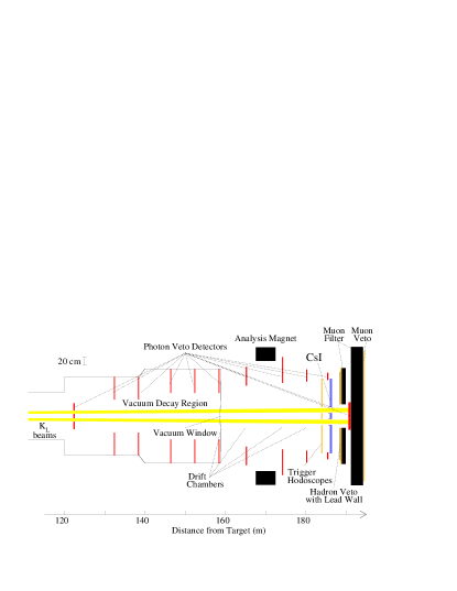
Figure 1: The KTeV Detector, as configured for collecting the data used in this analysis.

The $K_{L}$ beams used in this experiment were produced by an 800 GeV beam of protons striking a beryllium oxide target. Collimators and sweeping magnets downstream of the target produced two, nearly parallel neutral beams. The decay volume for accepted decays began 110 meters from the target to allow the $K_{S}$ component to decay away, and continued to the first drift chamber of the spectrometer at 160 meters. The acceptance for decays upstream of 122 meters was restricted by the “Mask Anti” (MA) anti-coincidence counter which had holes to allow the beams to pass. The kaon beams and decay products traveled through vacuum from the target to the first drift chamber.

The KTeV spectrometer measured the charged decays products. It consisted of four rectangular drift chambers, each with two horizontal and two vertical planes of sense wires, and a large dipole magnet which imparted a transverse momentum of 0.412 GeV/$c$. The drift chambers measured horizontal and vertical track position with a resolution of 110 $\mu$m and momentum with a resolution of 0.4% at a typical momentum of 36 GeV/$c$.

Energy measurements and particle identification were performed by a pure cesium iodide electromagnetic calorimeter (CsI). It consisted of 3100 blocks in a square array 1.9 m on a side and 0.5 m deep. Two 15 cm square beam holes allowed the passage of the neutral beams through the calorimeter. The calorimeter was calibrated using momentum-analyzed electrons, with average energy resolution for electrons of 0.75% (where the momentum resolution has not been subtracted out). The calorimeter was also used to associate tracks between vertical and horizontal views.

Following the CsI was a five meter long iron muon filter. Muons needed to have a momentum greater than 7 GeV/$c$ in order to traverse the filter and deposit energy in the veto scintillation plane.

A series of “photon veto” counters surrounded the fiducial volume of the detector to detect particles missing the CsI. These veto counters suppressed the background from $K_{L}\rightarrow\pi^{+}\pi^{-}\pi^{0}$ ($K_{\pi 3}$) and other decays with extra photons.

The data for this analysis were collected in a dedicated low intensity (10% of nominal $\epsilon^{\prime}/\epsilon$ intensity) run during a 24 hour period in 1997. The low intensity of these runs was crucial to having a manageable accidental background component to our measurement. Only minimal trigger conditions were applied: trigger hodoscope signals indicating the presence of at least two charged tracks, in anti-coincidence with photon veto counters.

III Analysis

The analysis of this decay proceeded in two stages. First, an inclusive $K_{e3}$ sample was isolated, then a subsample containing one photon was identified.

III.1 $K_{e3}$ Sample

The presence of an electron and a pion originating from a common vertex define the $K_{e3}$ normalization sample. Particle identification was performed by comparing the momentum measured by the spectrometer with the energy deposited in the calorimeter: the electron was required to have $0.95<E/P<1.1$; the pion, $E/P<0.7$. Events with extra tracks were rejected. The momentum of each track was required to be above 7 GeV in order to reject muons that stop in the muon filter before reaching the muon veto counter. Fiducial cuts were applied to tracks and clusters to restrict particles to well understood parts of the detector. Activity in the photon veto counters was not allowed (deposited energy $<0.3$ GeV), however, there was no cut on extra energy deposits in the CsI and photons could go down the beam hole without being detected. A plot of the charged particle momentum of the normalization $K_{e3}$ sample is shown in Figure 2 along with a Monte Carlo simulation of the same.

Figure 2: Data/MC comparisons of the total charged momenta ($P_{e\pi}$). The $\chi^{2}/{\rm DOF}=95.5/72.$

III.1.1 The Quadratic Ambiguity

We need to know the photon momentum in the CM for both the branching ratio and spectrum measurements. However, because the neutrino in $K_{e3}$ decays is unobserved, events cannot be reconstructed unambiguously. Kinematic constraints allow one to determine the magnitude of the neutrino’s CM momentum along the kaon flight direction but not the sign (forward or back). This leads to a two-fold ambiguity in determining the kaon’s lab momentum, and hence the photon’s CM momentum.

The acceptances for the two kaon lab momentum solutions are different, favoring one solution over the other. We picked the more likely solution for any pair of momenta based on MC calculations of the acceptance. This procedure resulted in the correct solution 65% of the time.

The quadratic ambiguity is smallest in cases where the neutrino emerges perpendicular to the kaon flight direction. Because of the finite resolution of the spectrometer, $\cos^{2}(\theta_{K\nu}^{*})$ can have non-physical, negative values. However, events in which the kaons scatter in the collimators can also have negative values of $cos^{2}(\theta_{K\nu}^{*})$. To retain most of the unambiguous events while rejecting large, unphysical values from events in which the kaon scattered, we required $\cos^{2}(\theta_{K\nu}^{*})>-0.2$.

III.1.2 Kinematic Cuts and Backgrounds

To increase the purity of the $K_{e3}$ sample, we required $P_{T}^{2}<0.055$ GeV² and $M_{e\pi}<0.5$ GeV, the kinematically allowed values.

$K_{\pi 3}$ events were a background at the tenth of a percent level in the $K_{e3}$ sample because of the small probability (0.3%) for a pion to be misidentified as an electron. $K_{\pi 3}$ events were more significant (a few percent) for the $K_{e3\gamma}$ subsample because the decay also has photons present. The mass of the unseen $\pi^{0}$ in $K_{\pi 3}$ decays, restricts the kinematics of the charged particles. By eliminating events in which the unobserved $\pi^{0}$ would have a physically allowed momentum when analyzed as $K_{\pi 3}$  we removed 99% of this background, while removing only 7% of the $K_{e3\gamma}$ signal.

Likewise, well over 99% of $K_{L}\rightarrow\pi^{+}\pi^{-}$ events with a misidentified pion were removed by cuts on the two pion invariant mass (494–502 MeV) and transverse momentum ($<50$ MeV²).

A few misreconstructed $K_{\pi 3}$ decays remained in the sample and were subtracted using a MC sample of $K_{\pi 3}$ events. This sample was normalized to the data in the case where the kinematic requirement above has been dropped and the signal had been estimated with a sample of MC $K_{e3}$ events. A small $K_{e4}$ background was also subtracted using a MC sample normalized to the inferred data kaon flux. These two subtractions together change the normalization sample by less than 0.1%.

III.2 $K_{e3\gamma}$ Subsample

The $K_{e3\gamma}$ subsample was selected from events in the inclusive $K_{e3}$ sample. The subsample consisted of events with exactly one photon candidate cluster.

The photon candidate cluster was required to be more than 8 cm from the electron cluster in the CsI and more than 40 cm from the pion cluster. The photon-electron distance cut allows for reliable separation of the electron and photon clusters. The photon-pion distance cut removed events in which clusters due to pion shower fluctuations, which are not well modeled in MC, might have mimicked a photon shower. The energy of a photon candidate cluster was required to exceed 3 GeV, while the transverse profile of the cluster was required to be consistent with the hypothesis of a single, electromagnetic shower. A plot of the photon energy in the laboratory frame is shown in Figure 3. The photon cluster was also required to be more than 2 cm away from the electron’s position as projected from the upstream track segment to the CsI. This cut removed photons from physical bremsstrahlung as the electron passed through the detector.

Figure 3: Data/MC comparisons of the photon energy in the laboratory frame at two different scales. The photon energy was required to be above 3 GeV to be included in the $K_{e3\gamma}$ sample. This cut is indicated by the vertical line in each plot. The $\chi^{2}/{\rm DOF}=6.2/14$ for the first plot and $24.4/27$ for the second.

The $K_{e3\gamma}$ events were required to have exactly one photon candidate cluster. In addition, the calorimeter was required to be free of other electromagnetic clusters with energy greater than 1 GeV and which were separated from the electron cluster by more than 4 cm and from the pion cluster by more than 30 cm. The MC does not simulate the multiplicity of these clusters perfectly. A small correction, $C_{V}$, of 0.25% was applied to account for this. The correction was determined by finding the ratio of the number of events with two or more photon candidate clusters to the number of events with one or more photon candidate clusters.

For the branching ratio measurement, additional kinematic cuts on the energy, $E_{\gamma}^{*}>30$ MeV, and the angle between the electron and photon in the CM, $\theta_{e\gamma}^{*}>20^{\circ}$, were used in order to obtain a result with a kinematic range commensurate with the previous experimental result and to emphasize the interesting kinematic region for DE studies.

In our study of the photon CM spectrum (see Section  VI), the cut on the distance between the photon candidate and the electron projection was lowered to 1 cm, to allow us to use looser kinematic cuts $E^{*}>25$ MeV and $\theta_{e\gamma}^{*}>5^{\circ}$.

The background subtractions mentioned above for the inclusive $K_{e3}$ sample were more significant in the $K_{e3\gamma}$ subsample, comprising 0.7% of the total.

IV Monte Carlo Simulation

The detector acceptance used in calculating the branching ratio and in determining the acceptance-corrected photon spectrum was calculated by MC simulation. As mentioned above, the photon momentum in $K_{e3\gamma}$ cannot be constrained due to the unseen neutrino. This ambiguity makes precise MC simulation essential to the success of this analysis. To accurately simulate accidental activity in the detector, a special trigger was used to record events at random times with a frequency proportional to the overall beam intensity. These random events were overlaid on MC generated events for comparisons with the data and for acceptance calculations. We were aided by the low beam intensity conditions under which the data were recorded.

FFSFFS:1970b present a full listing of all terms for the squared matrix element, including both IB and DE components. We used their listing explicitly in our Monte Carlo (MC) simulations. For the branching ratio measurement, all the DE coefficients were set to zero. The MC $K_{e3\gamma}$ sample was combined with a MC sample of non-radiative $K_{e3}$ decays at a level corresponding to NA31’s branching ratio measurementLeber:1996 . The cutoff for generating a physical photon to trace through the detector was 1 keV in the CM. Photons below this energy as well as loop effects were taken into account in the $K_{e3}$ generation. The $K_{e3}$ form factor, used for both radiative and non-radiative events was $\lambda_{+}=0.0274(14)$Tesarek:1999 , based on a preliminary KTeV measurement. Our result depends only weakly on the form factor, and the form factor used is in agreement with the 2000 PDG valuePDG:2000 .

Two other features of the MC simulation are worth mentioning. First, electromagnetic and hadronic showers in the CsI were handled by separate libraries of showers generated with GEANT. Second, the tracking of particles through the detector and beamline accounted for a number of effects including multiple scattering, bremsstrahlung and synchrotron radiation, delta particle emission, photon conversion and kaon regeneration.

V Branching Ratio Calculation

The measured relative branching ratio is simply defined by the ratio of the events we measure in each sample corrected by the acceptance in each case. It is important to realize that our dependence on MC is mitigated by the ratio of acceptances appearing in the calculation. The sample sizes and acceptances are listed in Table 1. Thus we find,

$$\frac{\Gamma(K_{e3\gamma},E_{\gamma}^{*}>30{\rm\ MeV},\theta_{e\gamma}^{*}>20^{\circ})}{\Gamma(K_{e3})}\\ =\frac{\rm N(K_{e3\gamma})}{\rm N(K_{e3})}\frac{\rm Acc(K_{e3})}{\rm Acc(K_{e3\gamma})}C_{V}\\ =0.908\pm 0.008({\rm stat})^{+0.013}_{-0.012}({\rm syst})\%$$ (2)

As mentioned above, the correction, $C_{V}=1.0025\pm 0.0009$, is necessary to take into account the different rates at which $K_{e3\gamma}$ candidate events are vetoed by the cluster multiplicity cut in data and MC. Vetoed events in the MC are not included in the MC calculation of the acceptance and thus require an explicit correction.

$$\begin{array}[]{lr}\hline\cr\hline\cr\lx@intercol\hfil{\rm Normalization,\ }K_{e3}\hfil\lx@intercol\\ \hline\cr{\rm RawEvents}&5760888\\ \qquad K_{\pi 3}{\rm\ background}&267\\ \qquad K_{e4}{\rm\ background}&197\\ {\rm Backgroundsubtractedevents}&5760424\\ K_{e3}{\rm\ Acceptance}&0.1067\\ \hline\cr\lx@intercol\hfil{\rm Signal,\ }K_{e3\gamma}(E_{\gamma}^{*}>30{\rm\ MeV},\theta_{e\gamma}^{*}>20^{\circ})\hfil\lx@intercol\\ \hline\cr{\rm RawEvents}&15575\\ \qquad K_{\pi 3}{\rm\ background}&50\\ \qquad K_{e4}{\rm\ background}&62\\ {\rm Backgroundsubtractedevents}&15463\\ K_{e3\gamma}{\rm Acceptance}&0.03161(14)\\ \hline\cr\hline\cr\end{array}$$

Table 1: Sample sizes used in the branching ratio calculation.

Our result is compared with the other published measurements and predictions in Figure 4. The uncertainties for the theoretical predictions are based solely on the accuracy of the stated results. FFS give a result only for $\theta_{e\gamma}^{*}>0$. We have used our MC (based explicitly on the FFS FFS:1970b matrix element) to calculate the fraction of the events with $\theta_{e\gamma}^{*}>20^{\circ}$ and give the result for this case.

Figure 4: A comparison of our branching ratio measurement with other recent measurements and predictions.

V.1 Systematic Uncertainties

Estimates of the sizes of various significant systematic uncertainties are listed in Table 2. The largest systematic uncertainty comes from the variation of the calculated branching ratio with the $E_{\gamma}$ cut, as the cut was varied by $\pm 1$ GeV about 3 GeV. Photons below 2 GeV are not well reconstructed as we have seen by analyzing large samples of $K_{\pi 3}$ decays. The relative size of this uncertainty reflects the steeply falling photon spectrum at low energies combined with the difficulty of modeling the calorimeter at the lowest energies.

The error associated with picking the right momentum solution was based on the degree of consistency between the subset of the data where momentum solution is unambiguous within resolution, and the data set as a whole. The error on the acceptance was based on the statistics of MC generated. To this was added the variation in acceptance due to the unknown DE parameters studied below. The upper limit on the background due to clusters originating from pion shower fluctuations was determined by studying $K_{\mu 3}$ decays in data.

The contribution of accidental activity in the CsI to the $K_{e3\gamma}$ subsample was small, 0.5%, as determined by generating MC with and without accidental overlays and comparing the number of events with exactly one photon candidate. The number of events with more than one photon candidate agreed between data and MC with accidental overlays at the 20% level, whereas there were differences of orders of magnitude without accidental overlays.

Other errors were estimated from the differences between data and MC shapes of various distributions combined with different expected shapes between normalization and signal samples, and the uncertainty in the measured $K_{e3}$ form factor.

$$\begin{array}[]{lrr}\hline\cr\hline\cr&{\rm Down(\%)}&{\rm Up(\%)}\\ \hline\cr E_{\gamma}{\rm\ cut}&-0.005&+0.008\\ K\ {\rm momentumsolution}&-0.007&+0.007\\ {\rm MCStatistics}&-0.006&+0.006\\ {\rm PionshowerBG}&-0.003&+0.000\\ K_{e3}\ {\rm formfactor}&-0.003&+0.003\\ P_{e}^{*}{\rm\ shape}&-0.003&+0.003\\ P_{T}^{2}{\rm\ shape}&-0.002&+0.002\\ {\rm VetoCorrection}&-0.001&+0.001\\ {\rm PhotonConversions}&-0.001&+0.001\\ \cos^{2}(\theta_{K\nu}^{*}){\rm\ shape}&-0.001&+0.001\\ {\rm AccidentalOverlay}&-0.001&+0.001\\ K_{\pi 3}\ {\rm BGsubtraction}&-0.001&+0.001\\ K_{e4}\ {\rm BGsubtraction}&-0.001&+0.001\\ \hline\cr{\rm TotalSystematicUncertainty}&-0.012&+0.013\\ {\rm StatisticalUncertainty}&-0.008&+0.008\\ \hline\cr{\rm TotalUncertainty}&-0.014&+0.015\\ \hline\cr\hline\cr\end{array}$$

Table 2: A list of significant uncertainties in the branching ratio measurement.

VI Spectrum Measurement

With the statistics available in this experiment, it becomes feasible to compare the FFS model for direct emission (Eq. (1)) with our observed photon CM momentum spectrum. We do not have the sensitivity to consider all four parameters, so we use the soft-kaon approximationHolstein:1999 to set $A=B=0$ and restricted our study to $C$ and $D$ whose terms remain non-zero in this approximation. The soft-kaon approximation assumes that terms in the decay matrix element proportional to the kaon rest mass are negligible.

To determine the values of $C$ and $D$ favored by our data, we used MC to generate spectra at a set of points in $CD$ space. We compared these spectra, bin-by-bin, to the acceptance-corrected spectrum seen in the data to calculate a $\chi^{2}$ value at each point. The only free parameter in this comparison was the normalization of the two spectra. To increase the statistics for these fits the photon-electron angle cut was relaxed to $\theta_{e\gamma}^{*}>5^{\circ}$. This cut is still far from allowing physical bremsstrahlung events into our sample. The fit was done for photon energies between 25 and 200 MeV in seven bins. Below 25 MeV we were limited by the sensitivity of our calorimeter to soft photons. Above 200 MeV, the error due to making the wrong kaon momentum choice became dominant.

The constant $\chi^{2}$ contours corresponding to $\sigma=1$ ($\chi^{2}-\chi_{\rm min}^{2}=1$) and $\sigma=2$ ($\chi^{2}-\chi_{\rm min}^{2}=4$) as a function of $C$ and $D$ are shown in Figure 5. A polynomial interpolation was done to estimate the values $\chi^{2}$ between sampled points. We find $C=-5\pm{10}$ and $D=5^{+19}_{-21}$, with a strong correlation between the two parameters.

Figure 5: The $\sigma=1$ ($\chi^{2}-\chi_{\rm min}^{2}=1$) and $\sigma=2$ ($\chi^{2}-\chi_{\rm min}^{2}=4$) contours of the fit/interpolated $\chi^{2}$ surface as a function of $C$ and $D$. The dot shows the position of the minimum, while the cross shows the IB-only point. The region within the oblique rectangle is rotated and redisplayed in the inset. The new axes $C^{\prime}$ and $D^{\prime}$ are obtained from $C$ and $D$ after a rotation of $\theta=25.8^{\circ}$.

We are most sensitive to the linear combination of $C$ and $D$ which approximates a linear perturbation of the IB-only spectrum. The precision of our result is more apparent when one chooses axes aligned with this combination. Choosing axes $C^{\prime}$ and $D^{\prime}$ rotated by $\theta=25.8^{\circ}$, we find $C^{\prime}=-2.5^{+1.5}_{-1.0}$ and $D^{\prime}=6^{+22}_{-24}$. This is illustrated in the inset of Figure 5.

The observed acceptance-corrected $E_{\gamma}^{*}$ spectrum is shown in comparison with the generated spectrum at the best-fit lattice point in Figure 6. The $\chi^{2}$ value for this point is 4.3 with four degrees of freedom. At the IB-only point (0,0), the $\chi^{2}$ is 7.4.

Figure 6: Data/MC comparison of the acceptance-corrected $E_{\gamma}^{*}$ spectrum at the best $CD$ point. The $\chi^{2}/{\rm DOF}=4.3/4$, where the 0–25 MeV bin has not been included in the comparison.

Knowledge of the acceptance correction is the dominant systematic error contributing to our measurement of $C^{\prime}$ and $D^{\prime}$. Physical backgrounds are very low and insignificant in the spectrum measurement. We estimated the systematic uncertainty associated with $C^{\prime}$ (the large statistical uncertainty in $D^{\prime}$ makes the systematic uncertainty insignificant) by multiplying the measured acceptance profile by a linear factor and renormalizing to keep the overall acceptance constant. The allowed size of the linear factor was determined by statistical consistency with the measured acceptance. By varying the acceptance in this manner we find a systematic uncertainty in $C^{\prime}$ of 1.5 and in $D^{\prime}$ of 1.0.

VII Conclusion

We have measured the relative branching ratio for radiative $K_{e3}$ decays and fit the photon spectrum to place limits on the size of DE components in the $K_{e3\gamma}$ matrix element. Our measurement, $\rm BR(K_{e3\gamma},E_{\gamma}^{*}>30{\rm\ MeV},\theta_{e\gamma}^{*}>20^{\circ})/\rm BR(K_{e3})=0.908\pm 0.008({\rm stat})^{+0.013}_{-0.012}({\rm syst})\%$, is nearly five times more precise than the previous measurement, and in agreement with it. It is significantly lower than all published theoretical predictions.

This is the first attempt to measure DE terms by studying the photon spectrum. The spectrum measurement is consistent with IB as the only source of photons in $K_{e3\gamma}$ decays. In the soft-kaon approximation, we find $C=-5\pm{10}$ and $D=5^{+19}_{-21}$, or, in a frame rotated by $25.8^{\circ}$, $C^{\prime}=-2.5^{+1.5}_{-1.0}({\rm stat})\pm 1.5({\rm syst})$ and $D^{\prime}=6^{+22}_{-24}\pm 1.0({\rm syst})$.

- (1) H. Fearing and J. Smith, Phys. Rev. 184, 1645 (1969).
- (2) H. Fearing et al., Phys. Rev. Lett. 24, 189 (1970).
- (3) H. Fearing et al., Phys. Rev. D 2, 542 (1970).
- (4) M. G. Doncel, Phys. Lett. 32B, 623 (1970).
- (5) B. R. Holstein, Phys. Rev. D 41, 2829 (1990).
- (6) J. Bijnens et al., Nucl. Phys. B369, 81 (1993).
- (7) F. Leber et al., Phys. Lett B 369, 69 (1996).
- (8) R. Tesarek, Scalar and tensor couplings in kaon decays (1999), hep-ex/9903069.
- (9) D. E. Groom et al., European Physical Journal C15, 1 (2000).
- (10) B. R. Holstein, private communication.