Improved Upper Limits on the FCNC Decays $B\rightarrow K\ell^{+}\ell^{-}$ and $B\rightarrow K^{*}(892)\ell^{+}\ell^{-}$

Abstract

We have searched a sample of 9.6 million $B\bar{B}$ events for the flavor-changing neutral current decays $B\rightarrow K\ell^{+}\ell^{-}$ and $B\rightarrow K^{*}(892)\ell^{+}\ell^{-}$. We subject the latter decay to the requirement that the dilepton mass $m_{\ell\ell}$ exceed 0.5 GeV. There is no indication of a signal. We obtain the 90% confidence level upper limits ${\cal B}(B\rightarrow K\ell^{+}\ell^{-})<1.7\times 10^{-6}$ and ${\cal B}(B\rightarrow K^{*}(892)\ell^{+}\ell^{-})_{m_{\ell\ell}>0.5{\rm GeV}}<3.3\times 10^{-6}$. We also obtain an upper limit on the weighted average $0.65{\cal B}(B\rightarrow K\ell^{+}\ell^{-})+0.35{\cal B}(B\rightarrow K^{*}(892)\ell^{+}\ell^{-})_{m_{\ell\ell}>0.5{\rm GeV}}<1.5\times 10^{-6}$. The weighted-average limit is only 50% above the Standard Model prediction.

S. Anderson,¹ V. V. Frolov,¹ Y. Kubota,¹ S. J. Lee,¹ R. Poling,¹ A. Smith,¹ C. J. Stepaniak,¹ J. Urheim,¹ S. Ahmed,² M. S. Alam,² S. B. Athar,² L. Jian,² L. Ling,² M. Saleem,² S. Timm,² F. Wappler,² A. Anastassov,³ E. Eckhart,³ K. K. Gan,³ C. Gwon,³ T. Hart,³ K. Honscheid,³ D. Hufnagel,³ H. Kagan,³ R. Kass,³ T. K. Pedlar,³ J. B. Thayer,³ E. von Toerne,³ M. M. Zoeller,³ S. J. Richichi,⁴ H. Severini,⁴ P. Skubic,⁴ A. Undrus,⁴ V. Savinov,⁵ S. Chen,⁶ J. W. Hinson,⁶ J. Lee,⁶ D. H. Miller,⁶ E. I. Shibata,⁶ I. P. J. Shipsey,⁶ V. Pavlunin,⁶ D. Cronin-Hennessy,⁷ Y. Kwon,^7, A.L. Lyon,⁷ W. Park,⁷ E. H. Thorndike,⁷ T. E. Coan,⁸ Y. S. Gao,⁸ Y. Maravin,⁸ I. Narsky,⁸ R. Stroynowski,⁸ J. Ye,⁸ T. Wlodek,⁸ M. Artuso,⁹ K. Benslama,⁹ C. Boulahouache,⁹ K. Bukin,⁹ E. Dambasuren,⁹ G. Majumder,⁹ R. Mountain,⁹ T. Skwarnicki,⁹ S. Stone,⁹ J.C. Wang,⁹ A. Wolf,⁹ S. Kopp,¹⁰ M. Kostin,¹⁰ A. H. Mahmood,¹¹ S. E. Csorna,¹² I. Danko,¹² K. W. McLean,¹² Z. Xu,¹² R. Godang,¹³ G. Bonvicini,¹⁴ D. Cinabro,¹⁴ M. Dubrovin,¹⁴ S. McGee,¹⁴ A. Bornheim,¹⁵ G. Eigen,^15, E. Lipeles,¹⁵ S. P. Pappas,¹⁵ A. Shapiro,¹⁵ W. M. Sun,¹⁵ A. J. Weinstein,¹⁵ D. E. Jaffe,¹⁶ R. Mahapatra,¹⁶ G. Masek,¹⁶ H. P. Paar,¹⁶ A. Eppich,¹⁷ R. J. Morrison,¹⁷ R. A. Briere,¹⁸ G. P. Chen,¹⁸ T. Ferguson,¹⁸ H. Vogel,¹⁸ J. P. Alexander,¹⁹ C. Bebek,¹⁹ B. E. Berger,¹⁹ K. Berkelman,¹⁹ F. Blanc,¹⁹ V. Boisvert,¹⁹ D. G. Cassel,¹⁹ P. S. Drell,¹⁹ J. E. Duboscq,¹⁹ K. M. Ecklund,¹⁹ R. Ehrlich,¹⁹ P. Gaidarev,¹⁹ L. Gibbons,¹⁹ B. Gittelman,¹⁹ S. W. Gray,¹⁹ D. L. Hartill,¹⁹ B. K. Heltsley,¹⁹ L. Hsu,¹⁹ C. D. Jones,¹⁹ J. Kandaswamy,¹⁹ D. L. Kreinick,¹⁹ M. Lohner,¹⁹ A. Magerkurth,¹⁹ H. Mahlke-Krüger,¹⁹ T. O. Meyer,¹⁹ N. B. Mistry,¹⁹ E. Nordberg,¹⁹ M. Palmer,¹⁹ J. R. Patterson,¹⁹ D. Peterson,¹⁹ D. Riley,¹⁹ A. Romano,¹⁹ H. Schwarthoff,¹⁹ J. G. Thayer,¹⁹ D. Urner,¹⁹ B. Valant-Spaight,¹⁹ G. Viehhauser,¹⁹ A. Warburton,¹⁹ P. Avery,²⁰ C. Prescott,²⁰ A. I. Rubiera,²⁰ H. Stoeck,²⁰ J. Yelton,²⁰ G. Brandenburg,²¹ A. Ershov,²¹ D. Y.-J. Kim,²¹ R. Wilson,²¹ B. I. Eisenstein,²² J. Ernst,²² G. E. Gladding,²² G. D. Gollin,²² R. M. Hans,²² E. Johnson,²² I. Karliner,²² M. A. Marsh,²² C. Plager,²² C. Sedlack,²² M. Selen,²² J. J. Thaler,²² J. Williams,²² K. W. Edwards,²³ A. J. Sadoff,²⁴ R. Ammar,²⁵ A. Bean,²⁵ D. Besson,²⁵ and X. Zhao²⁵

The flavor-changing neutral current (FCNC) decay $b\rightarrow s\ell^{+}\ell^{-}$ is sensitive to physics beyond the Standard Model[1], and, like the radiative penguin decay $b\rightarrow s\gamma$, is more amenable to calculation than purely hadronic FCNC decays. The decay $b\rightarrow s\ell^{+}\ell^{-}$ depends on the magnitude and sign of the three Wilson coefficients $C_{7}$, $C_{9}$, and $C_{10}$ in the effective Hamiltonian, while $b\rightarrow s\gamma$ depends only on the magnitude of $C_{7}$. These three Wilson coefficients are likely places for New Physics to appear, as they come from loop and box diagrams. Upper limits on the branching fraction for $b\rightarrow s\ell^{+}\ell^{-}$ thus place constraints on New Physics, while observation of $b\rightarrow s\ell^{+}\ell^{-}$ at a rate in excess of that predicted by the Standard Model would provide evidence for New Physics. Just as we first observed $b\rightarrow s\gamma$ through its exclusive decay $B\rightarrow K^{*}(892)\gamma$[2], and only later in an inclusive fashion[3], so we search for $b\rightarrow s\ell^{+}\ell^{-}$ through the decays $B\rightarrow K\ell^{+}\ell^{-}$ and $B\rightarrow K^{*}(892)\ell^{+}\ell^{-}$. Existing published upper limits come from CDF[4], and from earlier work by us[5]. Here we present improved upper limits.

The $B\rightarrow K^{*}\ell^{+}\ell^{-}$ decay rate peaks at low dilepton mass $m_{\ell\ell}$, due to the photon pole from $B\rightarrow K^{*}\gamma_{virtual},\ \gamma_{virtual}\rightarrow\ell^{+}\ell^{-}$. Because the decay $B\rightarrow K^{*}\gamma$ is already well studied, and $|C_{7}|$ thus reasonably well known, we require $B\rightarrow K^{*}\ell^{+}\ell^{-}$ candidates to have dilepton mass above 0.5 GeV, to reduce the contribution from the virtual photon diagram and thus the dependence on $|C_{7}|$.

The data used in this analysis were taken with the CLEO detector[6] at the Cornell Electron Storage Ring (CESR), a symmetric $e^{+}e^{-}$ collider operating in the $\Upsilon({\rm 4S})$ resonance region. The data sample consists of 9.2 ${\rm fb}^{-1}$ at the resonance, corresponding to 9.6 million $B\bar{B}$ events, and 4.5 ${\rm fb}^{-1}$ at a center-of-mass energy 60 MeV below the resonance. The sample below the resonance provides information on the background from continuum processes $e^{+}e^{-}\rightarrow q\bar{q},\ q=u,d,s,c$.

We search for $B\rightarrow K^{(*)}\ell^{+}\ell^{-}$ both in the $\mu^{+}\mu^{-}$ and $e^{+}e^{-}$ modes, for $B\rightarrow K\ell^{+}\ell^{-}$ in both the $K^{\pm}$ and $K^{0}$ modes, and for $B\rightarrow K^{*}\ell^{+}\ell^{-}$ in the $K^{*0}\rightarrow K^{+}\pi^{-}$ and $K^{0}\pi^{0}$ modes and in the $K^{*\pm}\rightarrow K^{\pm}\pi^{0}$ and $K^{0}\pi^{\pm}$ modes, a total of 12 distinct final states. $K^{0}$ is detected via the $K^{0}\rightarrow K^{0}_{S}\rightarrow\pi^{+}\pi^{-}$ decay chain.

There are three main sources of background: $B\rightarrow K^{(*)}\psi^{(\prime)},\ \psi^{(\prime)}\rightarrow\ell^{+}\ell^{-}$, and other $B\rightarrow\psi^{(\prime)}X$ decays; continuum processes with two apparent leptons (either real leptons or hadrons misidentified as leptons); and $B\bar{B}$ decays other than $B\rightarrow\psi^{(\prime)}X$, with two apparent leptons. We suppress $B\rightarrow K^{(*)}\psi^{(\prime)}$ events with vetoes on the dilepton mass around $\psi$ and $\psi^{\prime}$, in particular $2.80<m_{ee}<3.23$ GeV, $2.90<m_{\mu\mu}<3.20$ GeV, $3.51<m_{ee}<3.77$ GeV, and $3.55<m_{\mu\mu}<3.74$ GeV. These very wide cuts are needed because of the low-side radiative tail from internal and external bremsstrahlung from $\psi^{(\prime)}\rightarrow e^{+}e^{-}$, and to a lesser extent the low-side radiative tail from internal bremsstrahlung from the $\mu^{+}\mu^{-}$ decay.

We suppress the background from $B\bar{B}$ semileptonic decays with a cut on the event missing energy, $E_{miss}$, since events with leptons from semileptonic $B$ or $D$ decay contain neutrinos. Distributions in $E_{miss}$ for Monte Carlo samples of signal and background are shown in Fig. 1. We suppress continuum events with a cut on a Fisher discriminant, a linear combination of $R_{2}$ (the ratio of second and zeroth Fox-Wolfram moments[7] of the event), $\cos\theta_{tt}$ ($\theta_{tt}$ the angle between the thrust axis of the candidate $B$ and the thrust axis of the rest of the event), S (the sphericity), and $\cos\theta_{B}$ ($\theta_{B}$ the production angle of the candidate $B$, relative to the beam direction). In particular, ${\cal F}=R_{2}+0.117|\cos\theta_{tt}|+0.779(1-S)+0.104|\cos\theta_{B}|$. The coefficients of all terms but $R_{2}$ were determined by the standard Fisher discriminant procedure[8]. The relative weight given to $R_{2}$ was determined visually, from a scatter plot of $R_{2}$ vs. the Fisher discriminant from the other three variables. Distributions in ${\cal F}$ for Monte Carlo samples of signal and background are shown in Fig. 1.

For those decay modes involving a charged kaon, we use specific ionization ($dE/dX$) and time-of-flight information to identify the kaon, cutting loosely (3 standard deviations) if those variables deviate from the mean for kaons in the direction away from the mean for pions, and harder (by a variable number, denoted $kID^{cut}$, of standard deviations) if they deviate on the side towards the pions.

All cuts have been determined from Monte Carlo samples: continuum events, $B\bar{B}$ events with no signal, and $B\bar{B}$ events with a $B\rightarrow K^{(*)}\ell^{+}\ell^{-}$ signal. We optimized cuts on ${\cal F}$, $E_{miss}$, and, where appropriate, kaon identification simultaneously. We found that the optimum curve in efficiency vs. background space was traced out if we required that cuts on ${\cal F}$, $E_{miss}$, and $kID$ were tightened or loosened together. In particular, we found that the optimum curve was well described by $E^{cut}_{miss}=1.0+6.67\times({\cal F}^{cut}-0.8)$ GeV, $kID^{cut}=3.0-0.66\times(3.0-E^{cut}_{miss})$. With this formulation, we have a single cut variable, ${\cal F}^{cut}$, to optimize.

We optimized the cuts to obtain either the best upper limit, assuming no signal, or to see the smallest possible signal. These two different optimization procedures led to similar cuts, and we took the average. In the optimization we allowed the value of ${\cal F}^{cut}$ to vary from decay mode to mode. The final cuts on ${\cal F}$ are shown in Table I. The corresponding cuts on $E_{miss}$ and $kID$ can be obtained from the expressions given above.

Our final discrimination between signal and background comes from the $B$ reconstruction variables conventionally used for decays from the $\Upsilon(4S)$, beam-constrained mass $M_{cand}\equiv\sqrt{E^{2}_{beam}-P^{2}_{cand}}$ and $\Delta E\equiv E_{cand}-E_{beam}$. Our resolution in $M_{cand}$ is 2.5 MeV, and in $\Delta E$, 20 MeV. We define a signal box in $M_{cand}-\Delta E$ space, $\pm$ 6.5 MeV around the $B$ mass by $\pm$ 60 MeV ($\mu^{+}\mu^{-}$) or $\pm$ 70 MeV ($e^{+}e^{-}$). The signal box for $e^{+}e^{-}$ events is shifted off zero by 5 MeV in $\Delta E$, because radiation losses cause $B\rightarrow K^{(*)}e^{+}e^{-}$ signal events to peak at –5 MeV in $\Delta E$ rather than at zero.

Background from $B\rightarrow\psi^{(\prime)}X$ is estimated from Monte Carlo simulation. Background from other $B$ decay processes and from continuum processes is determined using a large sideband region in $M_{cand}-\Delta E$ space: $5.20<M_{cand}<5.29$ GeV, $|\Delta E|<0.25$ GeV, but excluding the signal box. From Monte Carlo simulation, we found that the ratio of events in the signal region to events in the sideband region is 0.024 for $B\bar{B}$ background events other than $B\rightarrow\psi^{(\prime)}X$, and 0.027 for continuum background, in both cases smaller than the ratio of areas, 0.038, because backgrounds fall off as the candidate mass approaches the beam energy. Recognizing that this ratio must be larger for continuum background than for $B\bar{B}$ background because the more jet-like continuum events will not fall off as rapidly as candidate mass approaches beam energy, and recognizing that using a lower background in an upper limit computation gives a more conservative answer, we take the continuum scaling factor to be equal to the $B\bar{B}$ scaling factor, rather than using 0.027.

The $e^{+}e^{-}$ events suffer a degradation in resolution due to internal and external bremsstrahlung from the electrons. We partially recover that resolution by adding to each electron energy the energy of those photons found nearby in angle. This procedure improves the $\psi$ veto, and resolution in $E_{miss}$, $M_{cand}$, and $\Delta E$.

The number of events that satisfy all cuts and land in the signal box is given, for each mode, in Table I, along with the background estimate. We find 3 $B\rightarrow K\ell^{+}\ell^{-}$ candidates, with an expected background of 2.0; we find 4 $B\rightarrow K^{*}\ell^{+}\ell^{-}$ candidates, with an expected background of 3.8. Thus there are a total of 7 events with an expected background of 5.8. The probability that a true mean of 5.8 will fluctuate up to 7 or more events is 36%. Thus, there is no indication of signal. A scatter plot of $M_{cand}$ vs. $\Delta E$ for events passing all other cuts and landing in the signal or sideband region is shown in Fig. 2. Again, no indication of a signal. We obtain upper limits.

We calculate upper limits, at 90% confidence level, taking backgrounds into account[9]. To allow for the uncertainty in the background estimate, we use a value for the background which is reduced below our actual estimate. For individual modes, we use half the estimated background. For $B\rightarrow K\ell^{+}\ell^{-}$ and $B\rightarrow K^{*}\ell^{+}\ell^{-}$ totals, we use the estimated background minus 1.28 standard deviations of its combined statistical and systematic error. (The factor 1.28 gives a 90% confidence level lower estimate of the background, assuming its uncertainty has a Gaussian distribution.) Results are given in Table I.

We gain experimental sensitivity to the underlying $b\rightarrow s\ell^{+}\ell^{-}$ interaction by calculating a weighted average over the two decay modes studied. To account for the difference in the experimental precision for each mode, we weight them by our relative efficiencies, that is, we compute an upper limit on the sum over all the individual sub-modes. This gives an upper limit on $0.65{\cal B}(B\rightarrow K\ell^{+}\ell^{-})+0.35{\cal B}(B\rightarrow K^{*}\ell^{+}\ell^{-})$, where the coefficients 0.65 and 0.35 are the relative efficiencies we have for the two modes.

We use Monte Carlo simulation to determine the efficiency for detecting the signal modes. The decays $B\rightarrow K\ell^{+}\ell^{-}$ and $B\rightarrow K^{*}\ell^{+}\ell^{-}$ are generated using the model of Ali et al.[1]. The helicity of the $K^{*}$ is taken into account. Final-state radiation is included, using the CERNlib subroutine Photos[10]. We have also generated decays with the two extreme variations that Ali et al. suggest for their model, and with several other models[11, 1]. We find the model-to-model variation in efficiency to be small, with a relative r.m.s. variation of $\pm$3%.

To check our procedures, we have looked for the decays $B\rightarrow J/\psi K^{(*)}$ rather than vetoing them. We compare the branching fractions obtained with those from prior CLEO measurements. There is good agreement – differences are at or below the one-standard-deviation level.

Systematic errors are of two varieties – those on the estimate of signal detection efficiencies, and those on the estimate of backgrounds. The contributors to the former are lepton identification uncertainties (contributing $\pm$5%, relative, in the efficiency), missing-energy-simulation uncertainties ($\pm$3.5%), and simulation uncertainties for $M_{cand}$, $\Delta E$, $dE/dX$, time of flight, and ${\cal F}$ ($\pm$3.0%), giving a $\pm$7% relative uncertainty in the overall efficiency. To this we add in quadrature $\pm$3% for the model dependence of the efficiency, discussed earlier. The contributors to the background uncertainties are the modelling of $B\rightarrow\psi^{(\prime)}X$ ($\pm$10%), and uncertainties in the scale factors from sideband region to signal region in $M_{cand}\ -\ \Delta E$ space. We assign a systematic error to the $B\bar{B}$ background scale factor by determining it with different methods, obtaining 0.024 $\pm$ 0.004. Recognizing that the scale factor for continuum should be larger than that for $B\bar{B}$, we conservatively set it equal to the $B\bar{B}$ scale factor, with the same (correlated) systematic error. The errors shown on the backgrounds in Table I include statistical errors and the systematic errors just described.

There is no universally agreed-upon procedure for including systematic errors in upper-limit estimates. We conservatively reduce the background by 1.28 standard deviations, and decrease the efficiency by 1.28 standard deviations. In this way we obtain our final results:

$${\cal B}(B\rightarrow K\ell^{+}\ell^{-})<1.7\times 10^{-6}\ ,$$

$${\cal B}(B\rightarrow K^{*}(892)\ell^{+}\ell^{-})_{m_{\ell\ell}>0.5{\rm GeV}}<3.3\times 10^{-6}\ ,\ \ {\rm and}$$

$$0.65{\cal B}(B\rightarrow K\ell^{+}\ell^{-})+0.35{\cal B}(B\rightarrow K^{*}(892)\ell^{+}\ell^{-})_{m_{\ell\ell}>0.5{\rm GeV}}<1.5\times 10^{-6}\ ,$$

all at 90% confidence level. These results are significant improvements over previously published limits[4, 5].

The Standard Model values for these branching fractions, as given by Ali et al.[1], are $0.6\times 10^{-6}$ for ${\cal B}(B\rightarrow K\ell^{+}\ell^{-})$ and $1.8\times 10^{-6}$ for ${\cal B}(B\rightarrow K^{*}\ell^{+}\ell^{-})_{m_{\ell\ell}>0.5GeV}$, and thus $1.0\times 10^{-6}$ for the 0.65 / 0.35 weighted average. The limit on the branching fraction for $B\rightarrow K\ell^{+}\ell^{-}$ is therefore about three times its Standard Model prediction, the limit on the branching fraction for $B\rightarrow K^{*}\ell^{+}\ell^{-}$, subject to the requirement that $m_{\ell\ell}>0.5$ GeV, is about twice its Standard Model prediction, and the 0.65 / 0.35 weighted average is only 50% larger than its Standard Model prediction.

In summary, we have searched for the decays $B\rightarrow K\ell^{+}\ell^{-}$ and $B\rightarrow K^{*}(892)\ell^{+}\ell^{-}$. We find no indication of a signal, and obtain upper limits on the branching fractions. These limits are consistent with Standard Model predictions, but not far above them.

We gratefully acknowledge the effort of the CESR staff in providing us with excellent luminosity and running conditions. This work was supported by the National Science Foundation, the U.S. Department of Energy, the Research Corporation, the Natural Sciences and Engineering Research Council of Canada, the Texas Advanced Research Program, and the Basic Science program of the Korea Research Foundation.

mode	${\cal F}^{cut}$	observed	background	efficiency	${\cal B}\times 10^{6}$
		events			upper Lim.
$K^{0}e^{+}e^{-}$	0.938	1	0.10	0.053	7.6
$K^{0}\mu^{+}\mu^{-}$	0.925	0	0.21	0.041	7.8
$K^{+}e^{+}e^{-}$	0.925	1	0.95	0.165	2.3
$K^{+}\mu^{+}\mu^{-}$	0.850	1	0.74	0.111	3.4
$K\ell^{+}\ell^{-}$		3	1.99 $\pm$0.35	0.370	1.49
$K^{0}\pi^{+}e^{+}e^{-}$	0.925	0	0.35	0.019	12.8
$K^{0}\pi^{+}\mu^{+}\mu^{-}$	0.900	0	0.27	0.015	15.6
$K^{+}\pi^{0}e^{+}e^{-}$	0.800	3	0.27	0.015	46.0
$K^{+}\pi^{0}\mu^{+}\mu^{-}$	0.750	0	0.49	0.008	29.3
$K^{+}\pi^{-}e^{+}e^{-}$	0.925	1	0.97	0.071	5.0
$K^{+}\pi^{-}\mu^{+}\mu^{-}$	0.875	0	1.24	0.052	4.6
$K^{0}\pi^{0}e^{+}e^{-}$	0.900	0	0.11	0.007	35.8
$K^{0}\pi^{0}\mu^{+}\mu^{-}$	0.750	0	0.10	0.002	117.3
$K^{*}\ell^{+}\ell^{-}$		4	3.80$\pm$0.57	0.188	2.94
Sum		7	5.79$\pm$0.83	0.558	1.35

TABLE I.: Value of ${\cal F}^{cut}$, number of events observed in signal window, the expected background, efficiency, and upper limit on the branching fraction, for the 12 modes, and for $B\rightarrow K\ell^{+}\ell^{-}$, $B\rightarrow K^{*}\ell^{+}\ell^{-}$, and 0.65${\cal B}(B\rightarrow K\ell^{+}\ell^{-})+0.35{\cal B}(B\rightarrow K^{*}\ell^{+}\ell^{-})$. Note, the upper limits given in this table have been corrected for systematic error in background, but not corrected for the systematic error in efficiency.

FIG. 1.: Distributions in $E_{miss}$ (upper) and ${\cal F}$ (lower) for Monte Carlo samples of signal events (solid), $B\bar{B}$ background events (dotted), and continuum background events (dashed). The vertical scale is arbitrary.

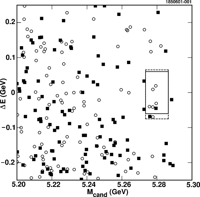
FIG. 2.: Scatter plot of $M_{cand}$ vs. $\Delta E$ for $ee$ events (open circles) and $\mu\mu$ events (solid squares) passing all other cuts, for data on the $\Upsilon(4S)$ resonance. The smaller box (solid) is the $\mu^{+}\mu^{-}$ signal box, while the larger box (dashes), shifted 5 MeV toward negative $\Delta E$, is the $e^{+}e^{-}$ signal box.

REFERENCES

- [1] A. Ali, P. Ball, L. T. Handoko, and G. Hiller, Phys. Rev. D 61, 074024 (2000) and references therein; C. Greub, A. Ioannissian, and P. Wyler, Phys. Lett. B 346, 149 (1995).
- [2] R. Ammar et al. (CLEO), Phys. Rev. Lett. 71, 674 (1993).
- [3] M. S. Alam et al. (CLEO), Phys. Rev. Lett. 74, 2885 (1995).
- [4] T. Affolder et al. (CDF), Phys. Rev. Lett. 83, 3378 (1999).
- [5] T. Skwarnicki, Proceedings of the XXIX Int. Conf. on High Energy Physics, Vancouver, Canada, 1998, edited by A. Astbury, D. Axen, and J. Robinson (World Scientific, Singapore, 1999), p. 1057; S. Glenn et al. (CLEO), Phys. Rev. Lett. 80, 2289 (1998).
- [6] Y. Kubota et al. (CLEO), Nucl. Instrum. Methods Phys. Res., Sect. A 320, 66 (1992); T. Hill, Nucl. Instrum. Methods Phys. Res., Sect. A 418, 32 (1998).
- [7] G. Fox and S. Wolfram, Phys. Rev. Lett. 41, 1581 (1978).
- [8] R. A. Fisher, Ann. Eugen. 7, 179 (1936); M. C. Kendall and A. Stuart, The Advanced Theory of Statistics, Second Edition (Hafner, New York, 1968) Vol III.
- [9] R. M. Barnett et al. (Particle Data Group), Phys. Rev. D 54 Part I, 1 (1996).
- [10] E. Barberio and Z. Was, Comput. Phys. Commun. 79, 291 (1994).
- [11] P. Ball and V. M. Braun, Phys. Rev. D 58, 094016 (1998); Patricia Ball, Journ. High Energy Phys., 9809, 005 (1998), hep-ph/9802394; D. Melikhov and N. Nikitin, hep-ph/9609503; P. Colangelo et al., Phys. Rev. D 53, 3672 (1996); erratum, Phys. Rev. D 57, 3186 (1998).