T24 Production at Intermediate Energies and Lund Area Law

Abstract

The Lund area law was developed into a Monte Carlo program LUARLW. The important ingredients of this generator was described. It was found that the LUARLW simulations are in good agreement with the BEPC/BES $R$ scan data between 2–5 GeV.

1 Introduction

The hadron production mechanism in particles collisions is one of the important subjects in the study of strong interaction. Quantum chromodynamics (QCD) is considered as the theory of strong interaction. However, the hadronization processes belong to nonperturbative problem for which no practicable calculation based on the first principle available. Some phenomenological hadronization models were thus built up, which play important roles in the studies toward the final understanding of strong interaction. The famous Lund string fragmentation model is one of the successful hadronization schemes, which contains several nontrivial dynamical features and describes the general semi-classical picture of hadron production. At high energies, the Lund generator, JETSET, can simulate the processes of hadron production via single photon annihilation and predicts the many properties of the final states correctly. But the application of Lund model at intermediate energies has been blank. A direct way out of this situation is to start from the basic assumptions of Lund model and find the solutions of the area law without adopting any high-energy approximation. Based on the Lund area law, a new generator LUARLW was compiled, which agrees with BES data between $2-5$ GeV well (see Figure 1 on page 1).

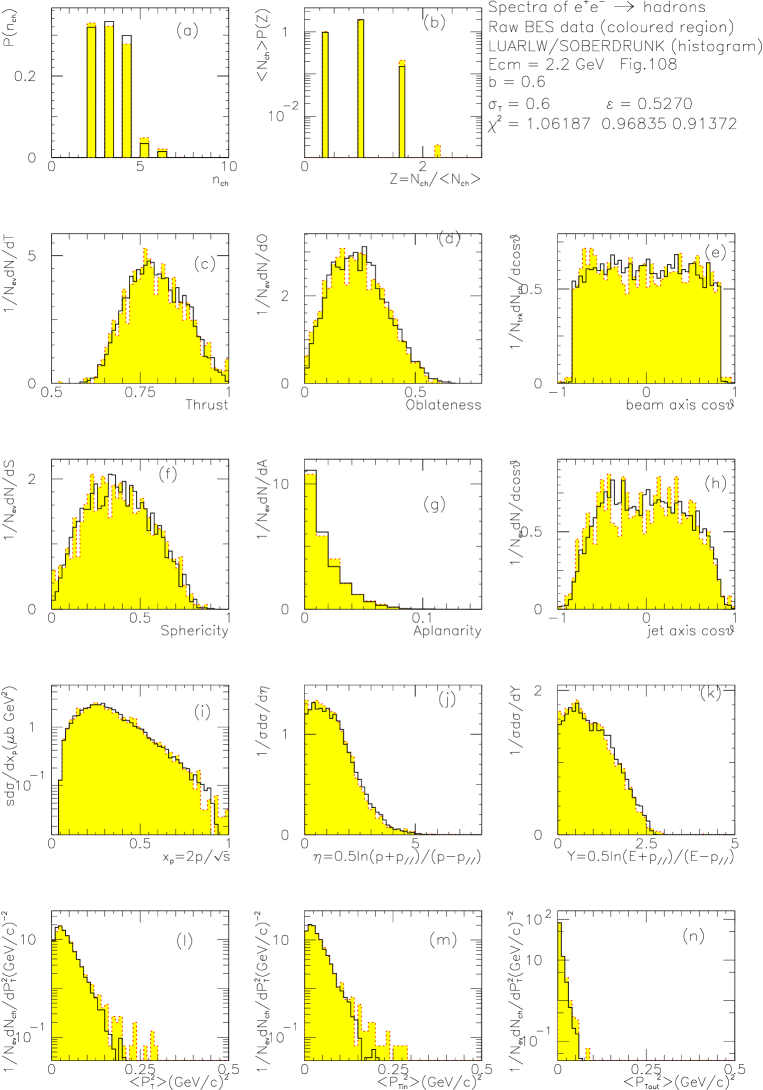
Figure 1: $e^{+}e^{-}\rightarrow$ hadrons spectrum of raw BES data (hatched region) and LUARLW/SOBDRUNK (black line) at $Ecm=2.2$ GeV.

2 Lund string fragmentation

The foundations of Lund model (relativity, causality and quantum mechanics) are universal. The basic hadron production picture is string fragmentation. The produced new pairs $(q\bar{q})$ and $(q\bar{q}q\bar{q})$ may form mesons and baryons if they carry with the correct flavor quantum numbers, otherwise they just behave like the vacuum fluctuations and do not lead any observable effects in experiments (see Figure 2).

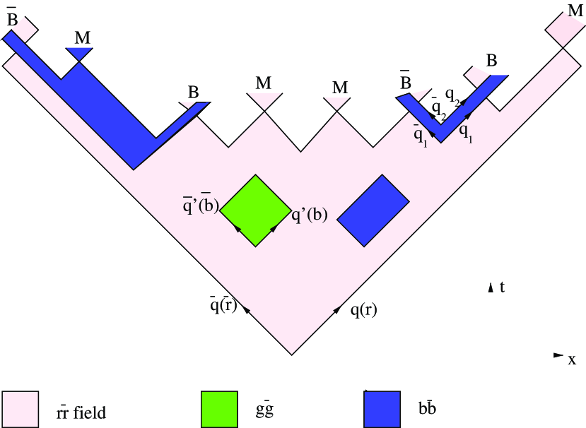
Figure 2: String fragmentation by a set of new pairs $(q\bar{q})$ and $(q\bar{q}q\bar{q})$ production, hadrons form at vertices

Using the assumptions of very high energy approximation (the remaining string always has large energy scale), left–right symmetry (fragmentation from $q_{0}$ end or $\bar{q}_{0}$ end are identical) and iterative fragmentation (string fragmentation may be treated iteratively), Lund fragmentation function $f(z)$ was derived uniquely,

$$f(z)=\frac{N}{z}(1-z)^{a}\exp\left(-\frac{bm^{2}}{z}\right),$$ (1)

where, $a$ and $b$ are fragmentation parameters, $m$ is the (transverse) mass of fragmentation hadron, and $z$ is the fraction of light-cone momentum. $f(z)$ is used in JETSET to govern string fragmentation. Lund fragmentation function $f(z)$ has the characteristics of inclusive distribution, and the single particle production is independent of anything else before and after. The applicable region of $f(z)$ is the remnant string still has large invariant mass. At intermediate energies, the mass-shell conditions should be the component part of the fragmentation dynamics, and the string usually fragments into $2\sim 6$ hadrons. Therefore the string fragmentation have to be treated as exclusive one instead of inclusive like in JETSET.

3 Lund area law

Lund string fragmentation process is Lorentz invariant and factorizable. The finite energy ($s$) system containing $n$ hadrons may be viewed as a cluster of infinite string fragmentation system with energy ($s_{0}\to\infty$) (see Figure 3). According to the general properties of iterative cascade, the combined distribution is the product of fragmentation functions for every steps

$$d\tilde{\wp}_{n} = \prod_{j=1}^{n}f_{j}(z_{j})dz_{j}$$ (2)

$$= C_{n}\cdot d\wp_{\mathrm{ext}}(s,z)\cdot d\wp_{n}(u_{1},\cdots,u_{n}),$$

where, $C_{n}$ is normalization constant. We know from (2) that a subsystem may be split up from the total system, the processes occurring in the subsystem is the same as it be a complete system starting at the some original energy $s$. The external part

$$d\wp_{\mathrm{ext}}(s,z)=ds\frac{dz}{z}(1-z)^{a}\cdot\exp(-b\Gamma)$$ (3)

corresponds to the probability that the cluster will occur. The internal part

$$d\wp_{n}(u_{1},\ldots,u_{n})=\delta^{2}\left(P_{n}-\sum_{j=1}^{n}p_{\circ j}\right)$$

$$\qquad\cdot\prod_{j=1}^{n}d^{2}p_{\circ j}\delta(p_{\circ j}^{2}-m_{\perp j}^{2})\exp(-b\mathcal{A}_{n})$$ (4)

then corresponds to the exclusive probability that the cluster will decay into the particular channel containing the given $n$ particles with energy-momentum $\{p_{\circ j}\}$ and nothing else. $\mathcal{A}_{\mathrm{rest}}=\mathcal{A}_{n}$ is the area enclosed by the quark and antiquark light-cone energy-momentum lines of $n$ particles.

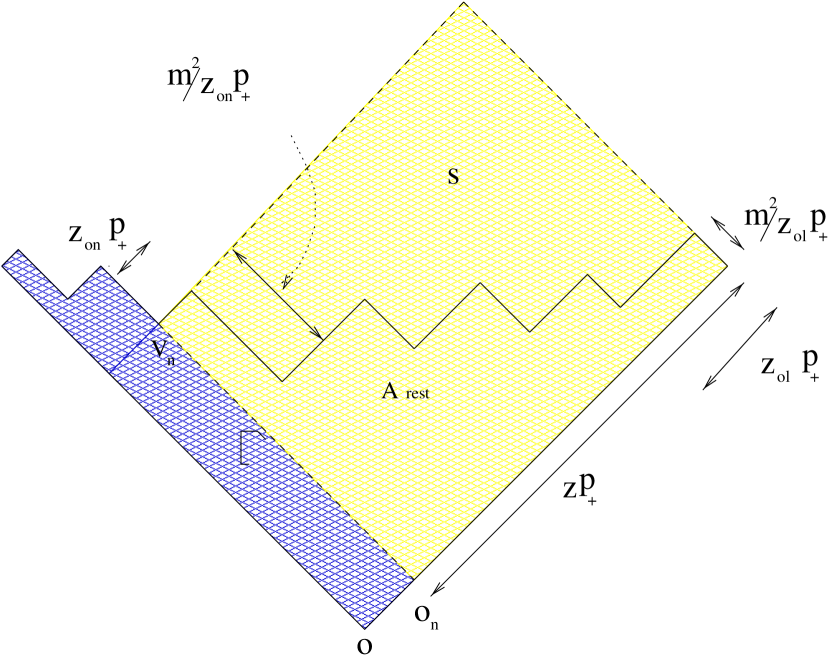
Figure 3: The situation after $n$ steps fragmentation.

The factor

$$|M|^{2}\equiv\exp(-b\mathcal{A}_{n})$$ (5)

may be viewed as the squared matrix element, the other parts are phase-space elements. In formulas, $b$ is fundamental color-dynamical parameters. Distribution (3) is called Lund area law. The total area

$$\mathcal{A}_{\mathrm{tot}}=\sum_{j=1}^{n}\mathcal{A}_{j}=\mathcal{A}_{n}+\Gamma,\qquad\Gamma=\frac{s(1-z)}{z}$$ (6)

and

$$\mathcal{A}_{n}=\sum_{j=1}^{n}\frac{m_{\perp j}^{2}}{z_{j}}\cdot\left(\sum_{k=j}^{n}z_{k}\right).$$ (7)

Finishing the integral over kinematic variables of $n-$particles, area law has following forms:

• String $\Rightarrow$ 2 hadrons

  $$\wp_{2}=\frac{C_{2}}{\sqrt{\lambda}}\left[\exp(-b\mathcal{A}_{2}^{(1)})+\exp(-b\mathcal{A}_{2}^{(2)})\right].$$ (8)

• String $\Rightarrow$ 3 hadrons

  $$d\wp_{3}=\frac{C_{3}}{\sqrt{\Lambda}}\exp(-b\mathcal{A})d\mathcal{A},$$ (9)

• String $\Rightarrow 4,5,6$ hadrons

  $$d\wp_{n}(s) = \frac{ds_{1}ds_{2}}{\sqrt{\lambda(s,s_{1},s_{2})}}\exp(-b\Gamma)$$ (10)

  $$\cdot \wp_{n_{1}}(s_{1},\mathcal{A}_{1})\wp_{n_{2}}(s_{2},\mathcal{A}_{2}).$$

In above fragmentation distributions, the gluon effects are neglected. At intermediate and low energies, the emitted gluons from initial quark or antiquark are usually soft, most of which will stop before the string starts to break, the effect of the gluon will then essentially be small transverse broadening of two-jet system, the gluon and quark will then look as single quark jet. The gluon emissions do not significantly change the topological shapes (sphericity and thrust) of final states, and therefore no observable jet effects.

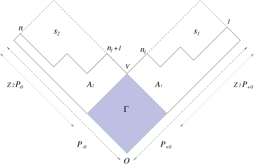
Figure 4: The vertex $V$ divides the $n$-body string fragmentation into two clusters which contain $n_{1}$ and $n_{2}$ hadrons and with squared invariant masses $s_{1}$ and $s_{2}$ separately.

4 Multiplicity

Lund area law may give the expression of the multiplicity distribution of fragmental hadrons. Define dimensionless $n$-particle partition function

$$Z_{n}=s\int dR_{n}\cdot\exp(-b\mathcal{A}),$$ (11)

where $dR_{n}$ is the $n$-particle phase space element. The relation between $Z_{n}$ and the multiplicity distribution $\tilde{P}_{n}$ for primary hadrons is

$$\tilde{P}_{n}=\frac{Z_{n}}{\sum Z_{n}}.$$ (12)

$\tilde{P}_{n}$ has the approximative expression

$$\tilde{P}_{n} = \frac{\mu^{n}}{n!}\cdot\exp[c_{0}+c_{1}(n-\mu)$$ (13)

$$\qquad+c_{2}(n-\mu)^{2}],\qquad(c_{2}<0).$$

Quantity $\mu$ may written as the energy-dependent form phenomenologicaly

$$\mu=a+b\cdot\exp(c\sqrt{s}),$$ (14)

or

$$\mu=a+b\ln(s)+c\ln^{2}(s).$$ (15)

All parameters $a$, $b$, $c$, $c_{0}$, $c_{1}$, and $c_{2}$ need to be determined by experimental data and have been tunned with BES data samples of $R$ scan.

5 Exclusive distribution

There are some different production channels for $n$-particle states, such as 4-body states may be $\pi^{+}\pi^{-}\pi^{+}\pi^{-}$, $\pi^{+}\pi^{-}\pi^{\circ}\pi^{\circ}$, $\rho^{+}\rho^{-}\pi+\pi^{-}$, etc. The exclusive probability for the special channel is

$$\hat{P}_{n}=B_{n}\cdot(VPS)\cdot(SUD)\cdot\wp_{n}(m_{\perp 1},\ldots,m_{\perp n};s).$$ (16)

• $B_{n}$ is the combinatorial number stemming from may be more than one string configurations lead to this state.

• (VPS) is the vector to pseudoscalar rate.

• (SUD) is the strange to up and down quark pair probability.

6 Transverse momentum distribution

Above results are obtained when the transverse momentums of all primary hadrons have given. In LUARLW, two transverse momentum distributions were used alternatively.

6.1 Scheme I

In Lund model, quantum mechanical tunneling effect is was used to explain the production of new pairs $q_{i}\bar{q}_{i}$. Particles obtain their transverse momenta from the constituents. At each production point the $(q_{i}\bar{q}_{i})$-pair is given $\pm{\bf q}_{i}$ and the particle momenta are

$$\mathbf{p}_{\perp 1}=\mathbf{q}_{1},\ldots\mathbf{p}_{\perp j}=\mathbf{q}_{j}-\mathbf{q}_{j-1},\ldots\mathbf{p}_{\perp n}=-\mathbf{q}_{n}.$$ (17)

Based on the Lund model, the following distribution with forward–backward symmetric correlation was derived

$$F^{(n)}(\mathbf{q}_{1},\ldots,\mathbf{q}_{n})$$

$$=C_{n}\exp\left\{-\frac{1}{2\sigma^{2}}\left[\mathbf{q}_{1}^{2}+\frac{(\mathbf{q}_{2}-\rho_{2}\mathbf{q}_{1})^{2}}{1-\rho_{2}^{2}}\cdots\right]\right\}$$

$$=C_{n}\exp\left\{-\frac{1}{4\sigma^{2}}\left[\mathbf{q}_{1}^{2}+\mathbf{q}_{n}^{2}\vphantom{\sum}\right.\right.$$

$$\qquad\left.\left.+\sum A_{j}(\mathbf{q}_{j}^{2}+\mathbf{q}_{j-1}^{2}-2\varepsilon_{j}\mathbf{q}_{j}\cdot\mathbf{q}_{j-1})\right]\vphantom{\frac{1}{4\sigma^{2}}}\right\},$$

with

$$A_{j}=\frac{(1+\rho_{j}^{2})}{(1-\rho_{j}^{2})},\qquad\varepsilon_{j}=\frac{2\rho_{j}}{(1+\rho_{j}^{2})}.$$ (18)

The correlations $\rho_{j}$ are phenomenological parameters, which in general are small. The covariant matrices

$$V_{2} = \sigma^{2}\left(\begin{array}[]{cc}1&\rho_{2}\\ \rho_{2}&1\end{array}\right),$$

$$V_{3} = \sigma^{2}\left(\begin{array}[]{ccc}1&\rho_{2}&\rho_{2}\rho_{3}\\ \rho_{2}&1&\rho_{3}\\ \rho_{2}\rho_{3}&\rho_{3}&1\end{array}\right),$$

$$V_{n} =$$

$$\sigma^{2}\left(\begin{array}[]{cccc}1&\rho_{2}&\cdots&\rho_{2}\rho_{3}\cdots\rho_{n}\\ \rho_{2}&1&\cdots&\rho_{3}\cdots\rho_{n}\\ \cdots&\cdots&\cdots&\cdots\\ \rho_{2}\cdots\rho_{n-1}&\rho_{3}\cdots\rho_{n-1}&\cdots&\rho_{n}\\ \rho_{2}\cdots\rho_{n}&\rho_{3}\cdots\rho_{n}&\cdots&1\end{array}\right)$$

give the correlations $\langle p_{xi}p_{xj}\rangle$ and $\langle p_{yi}p_{yj}\rangle$.

6.2 Scheme II

An available Gaussian-like transverse momentums distribution as options in LUARLW for $n-$particles fragmentation reads

$$F^{(n)}(\mathbf{p}_{\perp 1},\ldots,\mathbf{p}_{\perp n}) = \delta\left(\sum\limits_{j=1}^{n}\mathbf{p}_{\perp j}\right)$$ (22)

$$\theta\left(\sqrt{s}-\sum_{j=1}^{n}\sqrt{m_{j}^{2}+\mathbf{p}_{\perp j}^{2}}\right)$$

$$\cdot\prod_{j=1}^{n}\exp\left(-\frac{\mathbf{p}_{\perp j}^{2}}{2\sigma^{2}}\right).$$

The conditional distribution of $\mathbf{p}_{\perp 1}$, $\mathbf{p}_{\perp 2},\ldots,\mathbf{p}_{\perp j}$ are

$$f_{1}^{(n)}(\mathbf{p}_{\perp 1}) = N_{1}\cdot\exp\left[-\frac{n}{n-1}\frac{\mathbf{p}_{\perp 1}^{2}}{2\sigma^{2}}\right],$$

$$f_{2}^{(n)}(\mathbf{p}_{\perp 2}) = N_{2}\exp\left[-\frac{n-1}{n-2}\frac{(\mathbf{p}_{\perp 2}+\frac{\mathbf{p}_{\perp 1}}{n-1})^{2}}{2\sigma^{2}}\right],$$

$$f_{j}^{(n)}(\mathbf{p}_{\perp j}) =$$

$$N_{j}\exp\left[-\frac{(n-j+1)}{(n-j)}\frac{(\mathbf{p}_{\perp j}+\sum_{i=1}^{j-1}\frac{\mathbf{p}_{\perp j}}{n-j+1})^{2}}{2\sigma^{2}}\right].$$

The final $\mathbf{p}_{\perp n}$ is determined by energy-momentum conservation.The effective variance of $\mathbf{p}_{\perp j}$ is

$$\sigma_{j}^{\mathrm{(eff)}}=\sqrt{\frac{n-j}{n-j+1}}\sigma,\qquad(j=1,\ldots,n-1).$$ (23)

The transverse momentum distribution in this scheme is not exact Gaussian type due to the transverse momentum conservation and the threshold conditions.

7 Summary

The well-know Monte Carlo simulation packet JETSET is not built in order to describe few-body states at the few GeV level in $e^{+}e^{-}$ annihilation as at BEPC. We develop the formalism to use the basic Lund Model area law directly for Monte Carlo program LUARLW, which will be satisfied to treat two-body up to six-body states. In LUARLW, the effects of all gluonic emissions were neglected. The LUARLW predicts more than 14 distributions totally agree with BES data well.

Acknowledgement

This work was done under the instruction by Prof. Bo Andersson. All the knowledge about Lund model may be fond in The Lund Model by Bo Andersson, Cambridge University Press, Cambridge, 1998.