The Drift Chambers Of The Nomad Experiment

Abstract

We present a detailed description of the drift chambers used as an active target and a tracking device in the NOMAD experiment at CERN. The main characteristics of these chambers are a large area ($\rm 3\times 3~{}m^{2}$), a self supporting structure made of light composite materials and a low cost. A spatial resolution of $\rm 150~{}\mu m$ has been achieved with a single hit efficiency of $97\%$ .

Contents

1	Introduction	2
2	The drift chamber layout	3
3	The drift chamber electronics	10
4	The drift chamber construction	13
5	Gas system and slow control	17
6	The drift chamber performances	18
7	The drift chamber reconstruction software	25
8	Check of the drift chamber performances using experimental data	35
9	Conclusions	40
	Acknowledgements	40
	References	40

1 Introduction

The NOMAD experiment [1] was built to search for $\rm\nu_{\mu}\rightarrow\nu_{\tau}$ oscillations in the CERN SPS neutrino beam predominantly composed of $\rm\nu_{\mu}$’s with a mean energy of 24 GeV. The search [2] was based on the identification of $\rm\tau$’s produced by $\rm\nu_{\tau}$’s charged current (CC) interactions: $\rm\nu_{\tau}+N\rightarrow\tau^{-}+X$.
Given the $\rm\tau$ lifetime and the average energy of the CERN SPS neutrino beam, $\rm\tau$’s travel about 1 $\rm mm$ before decaying.
The spatial resolution of the NOMAD detector, though good, is not sufficient to resolve such short tracks. Instead, the decaying $\rm\tau$’s are identified through the kinematics of their decay products. The presence of at least one neutrino in the final state allows using momentum balance in the plane perpendicular to the neutrino beam direction in order to select $\rm\nu_{\tau}$ CC interaction candidates in a copious $\rm\stackrel{{\scriptstyle(-)}}{{\nu}}_{e,\mu}$ CC and NC background [3]. By studying correlations between the sizes and directions of three vectors in the transverse plane ($\rm\vec{p}_{T}^{\ miss}$, $\rm\vec{p}_{T}^{\ lepton}$ and $\rm\vec{p}_{T}^{\ hadrons}$) one can distinguish events containing $\tau^{-}$ decays from different sources of background, provided that the event kinematics is well reconstructed. This method of oscillation search therefore necessitated an excellent quality of measurement of all the secondary particles produced in the neutrino interactions and identification of electrons and muons. This was made possible thanks to an active target located inside a dipole magnet [4], and consisting of a set of large drift chambers, providing at the same time the neutrino target material and the charged particles tracker. Given this dual role, the chambers had to meet two conflicting requirements: their walls had to be as massive as possible in order to maximize the number of neutrino interactions and as light as possible to limit multiple scattering, secondary particle interactions and photon conversions. These conditions imposed the use of a low $Z$ material with good mechanical properties, mainly composite plastic materials.
The end result of the various necessary compromises was a target of 2.7 tons fiducial mass over a total volume of $\rm 2.6\times 2.6\times 4.5~{}m^{3}$. This gave a low average density of about 0.1 $\rm g/cm^{3}$ and less than 1% of a radiation length between two consecutive measurements.

The NOMAD detector was built over a period of 4 years starting in 1991 and was in operation during the next 4 years from 1995 to 1998. This paper is devoted to a description of the drift chambers used in this experiment.

2 The drift chamber layout

2.1 Introduction

The use of drift chambers for large detection areas appears to be the best solution for the reconstruction of charged particle trajectories. The event rate in neutrino experiments is such that no serious problem of pile-up can occur. The main requirement for the physics studied in NOMAD was to have a high density of coordinate measurements with good spatial resolution in order to apply the kinematic selection method described above, as well as to obtain a good determination of the neutrino interaction point and to be able to distinguish an electron from $\rm\tau$ decay from a converted gamma ray. The traditional solution is to weave wires over a rigid frame in order to produce the drift field. In our case the overall dimensions were limited by the internal size of the available magnet. Rigid frames would have reduced further the active area. The retained solution uses rigid panels of composite material on which glued aluminium strips produce the shaping field in the drift cell. Each chamber consists of three measurement planes allowing the reconstruction of one space point.

2.2 General overview

The fiducial volume of the NOMAD detector [5] consists of 44 drift chambers which act both as a low-density target and a tracking device. It is placed in a dipole magnet of internal volume $\rm 7\times 3.5\times 3.5~{}m^{3}$ operated at 0.4 Tesla. A sideview of the NOMAD detector is shown in figure 1. The magnetic field direction which is horizontal and orthogonal to the beam axis has been chosen as the X reference axis. The vertical axis is called the Y reference axis and the Z axis is obtained by the vectorial product of the X and Y directions (see figure 1). Downstream of the 4 m long target, 5 extra drift chambers are inserted in between the modules of the transition radiation detector (TRD) [6] in order to complete the tracking down to the preshower detector placed in front of the electromagnetic calorimeter [7], and to improve the momentum measurement resolution.

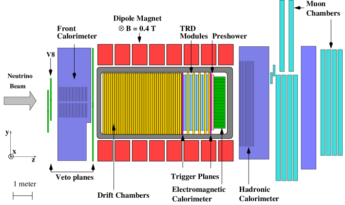
Figure 1: A sideview of the NOMAD detector. Z axis is horizontal and nearly coincides with the neutrino beam direction. Y axis is vertical and points to the top of the figure. X axis is along the magnetic field direction.

Figure 2: A sideview of one NOMAD drift chamber cut by a plane orthogonal to the X axis.

Each drift chamber has an active area of about $\rm 3~{}m$ by $\rm 3~{}m$ and consists of four panels enclosing 3 drift gaps of $\rm 8~{}mm$ (see figure 2) filled with an $\rm Ar(40\%)-C_{2}H_{6}(60\%)$ gas mixture at atmospheric pressure. The central gap (Y plane) is equipped with 44 sense wires parallel to the X axis and the outer gaps have 41 wires at $\rm-5^{\circ}$ (U plane) and $\rm+5^{\circ}$ (V plane) with respect to the X axis. For a high momentum track crossing the chambers along the Z axis the Y coordinate is obtained from the Y plane whereas the X coordinate is calculated combining the U and V plane measurements. Because of the small stereo angle, the resolution in X is about 10 times worse than the one in Y.

We start from a mechanical description of the drift chambers, while a detailed description of the drift cell will be given in subsection 2.5 (figure 4).

2.3 The panels

The design was studied in order to get self supporting chambers which act as a neutrino target. The challenge was to obtain a rigid and flat surface of $\rm 3\times 3~{}m^{2}$ which is at the same time as “transparent” as possible to particles and massive enough to yield a significant number of neutrino interactions. For these reasons, the panels have a composite sandwich structure of low Z materials. Each of them is composed of two $\rm 0.5~{}mm$ kevlar-epoxy ($\rm 0.57~{}kg/m^{2}$) skins surrounding an aramid honeycomb core structure ($\rm 32~{}kg/m^{3}$, 15 $\rm mm$ thick). Other solutions like polystyrene skins with rohacell or polystyrene foam have been tested and excluded because of rigidity and flatness considerations, although both solutions worked for small area (less than 3 $\rm m^{2}$) prototypes.

The total amount of material in each panel corresponds to 0.5% of a radiation length. The total thickness of a chamber is about $\rm 10~{}cm$ in Z and each chamber contributes 2% of a radiation length. The total fiducial mass (including the glue and the strips) of the 44 chambers is 2.7 tons over an area of $\rm 2.6\times 2.6~{}m^{2}$. The target is nearly isoscalar ($\rm N_{protons}\ :\ N_{neutrons}\ =\ 52.4\%\ :\ 47.6\%$). The material composition is shown in table 1.

Atom	prop./weight (%)	protons (%)	neutrons (%)
C	64.30	32.12	32.18
H	5.14	5.09	0.05
O	22.13	11.07	11.07
N	5.92	2.96	2.96
Cl	0.30	0.14	0.16
Al	1.71	0.82	0.89
Si	0.27	0.13	0.14
Ar	0.19	0.09	0.10
Cu	0.03	0.01	0.02
Total	99.99	52.43	47.56

Table 1: Drift chamber composition by weight (in percent).

The panel structure is reinforced by replacing locally the honeycomb with melamine inserts in the center and at the corners. 9 spacers ($\rm 10~{}mm$ in diameter) placed between two panels maintain the $\rm 8~{}mm$ drift gap. Nine insulated screws, $\rm 2~{}mm$ in diameter, cross the chambers in the center of the spacers in order to reinforce the whole structure. Four $\rm 10~{}mm$ diameter screws go through the whole chamber (one at each corner) and are used both for chamber assembly and panel positioning.

2.4 The drift field strips

To form an appropriate electric field in the drift cells, a polyester skin with aluminium strips is glued on each side of a drift gap. The strips are $\rm 2.8~{}mm$ wide, $\rm 12~{}\mu m$ thick and separated by a $\rm 1.2~{}mm$ gap large enough to avoid any sparking due to potential differences between strips. The sparking potential difference is 2200 V whereas the applied potential difference between adjacent strips is 400 V. The strips are obtained by a serigraphic technique. Ink is deposited on an aluminized polyester band with a 144 strip pattern. The band is then chemically treated in order to remove the aluminium between the strips. Finally the ink is washed off. The 5 strip bands needed to cover the full plane are tilted as the wires, with respect to the X axis by $\rm-5^{\circ}$, $\rm 0^{\circ}$ and $\rm+5^{\circ}$ depending on the drift gap. A gas-tight frame of bakelized paper, $\rm 4~{}mm$ thick, is glued on the panel to close the drift gap. At one end the strips go beyond the frame and the 16 strips corresponding to each drift cell (see subsection 2.5) are connected to a flexible high voltage bus using staples (see figure 3). The 6 HV buses of each chamber are connected to a high voltage distribution board located at the bottom of the chamber (see figure 4). Each pair of HV buses corresponding to a drift plane has its own resistor chain connected to a HV power supply. For the U and V planes ($\rm-5^{\circ}$ and $\rm+5^{\circ}$) a triangular zone of $\rm 25~{}cm$ by $\rm 3~{}m$ is left unequipped and is covered with glue in order to avoid any gas leaks through the panel. The residual distribution of the measured strip band positions with respect to the design values has an RMS of $\rm 250~{}\mu m$ and the positioning accuracy has been kept better than $\rm 500~{}\mu m$. We tried two methods for gluing of the strip bands. The first one was to use adhesive techniques because of easy manipulation during the construction. We tested the stability with time of this gluing technique in a vessel filled with an $\rm Ar(40\%)-C_{2}H_{6}(60\%)$ gas mixture during more than 2 years. This test was also used to check the aging of different materials (polystyrene, kevlar, rohacell, etc.). No change was observed. However, chambers built with this technique suffered from short circuits after several weeks of operation. Opening the chambers, we saw gas bubbles between the panels and the strip bands. This is probably due to the moisture gradient between the outside of the chamber and the dry gas in the drift gap. About 25 chambers suffered from the problem and they had to be modified both at Saclay and in a special workshop set up at CERN. The final gluing technique used a bi-component polyurethane glue to provide a stronger and more reliable attachment of the strip bands.

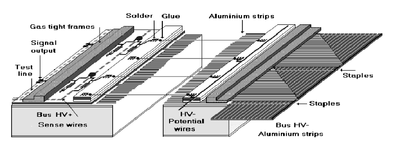
Figure 3: A cut view of a panel equipped as a Y plane.

2.5 The drift cells

The $\rm 20~{}\mu m$ diameter gold-plated tungsten sense wires placed in the center of the drift cells are held at a typical voltage of $\rm+1750~{}V$ through a $\rm 4.7~{}M\Omega$ resistor (see figure 4). The corresponding gain is of the order of $10^{5}$. The sense wire signal is readout by a preamplifier located on a board connected directly to the chamber printed board and AC coupled through a $\rm 1~{}nF$ capacitor. The preamplifier signal goes through a discriminator and is sent via a $\rm 30~{}m$ long cable to the TDC’s (see section 3). A test line located on the chamber printed board outside of the gas tight frames (see figure 3) allows to inject a signal just at the entrance of the amplifiers for test purposes.

Two Cu-Be potential wires, $\rm 100~{}\mu m$ in diameter, are placed at a distance of $\rm\pm 32~{}mm$ with respect to the sense wire and held at $\rm-3200~{}V$ (see figure 4) through a $\rm 10~{}M\Omega$ resistor which is shared by all potential wires of a drift plane.

The strips directly in front of the sense wires are grounded whereas those in front of the potential wires are held at $\rm-3200~{}V$. The strips in-between have a potential equally distributed so that the drift field perpendicular to the sense wire is of the order of $\rm 1~{}kV/cm$ in most of the cell (see figure 5). The measured drift velocity is approximately $\rm V_{drift}=50~{}\mu m/ns$ as expected from [8]. However, close to the sense and potential wires, the drift field changes drastically introducing non-linearities in the time to distance relation which are taken into account as second order corrections.

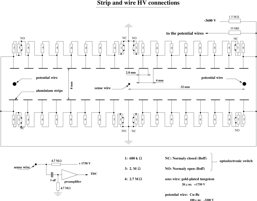
Figure 4: A close-up of a drift cell and its HV connections.

Since the drift chambers have to be operated inside a magnet delivering a field of 0.4 Tesla, the drift direction is tilted due to the Lorentz force. This effect is compensated for by shifting the potential on opposite strips by $\rm\pm 100$ V [9, 10] (see figure 5). Field configurations for field on and field off operation modes are obtained through an optoelectronic switch located on the HV distribution board (see figure 4).

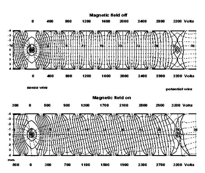
Figure 5: Potential and field lines along the drift cell for the two modes of operation: field OFF (top) and field ON (bottom).

The 3 $\rm m$ long potential and sense wires are soldered and glued at both ends (see figure 3) with a precision of about $\rm 100~{}\mu m$. Since the time to distance relation is extremely sensitive to the relative position of the wires with respect to the strips, the dominant error comes from the strip positioning. The final knowledge of the wire position in the experiment will be the result of a software alignment procedure described in section 6: in order to reduce the gravitational and electrostatic sagitta, the wires are glued on 3 epoxy-glass rods of 5 $\rm mm$ width which are in turn glued (parallel to the Y axis) over the strips. The free wire length is therefore reduced by a factor of 4 at the price of three dead regions, each less than $\rm 1~{}cm$ wide. To avoid having the dead regions aligned in the detector, the positions of the support rods are staggered along X by $\rm-5~{}cm$ (U plane), $\rm 0~{}cm$ (Y plane) and $\rm+5~{}cm$ (V plane).

2.6 The gas supply

The argon-ethane mixture is provided from the bottom of each chamber at 3 millibars above atmospheric pressure by two plastic pipes (one at each chamber side). The gas enters a $\rm 20~{}mm$ diameter distribution pipe which goes across the chamber. At each drift plane, the gas diffuses through $\rm 5~{}mm$ holes into the gap. On top of the chamber a similar system collects the gas. The gas tightness of each drift gap is ensured by inserting a string of polymerized silicon joint between the two frames. A second method using clamps and elastic o-ring joints has been tested and also used. The gas leaks were slightly higher with this method.

2.7 The chambers and modules

In each drift cell, the hit position ($\rm d_{h}$) with respect to the wire is obtained using the measured drift time ($\rm t_{d}$) and the time to distance relation ($\rm d_{h}=V_{drift}\times t_{d}$ in first approximation). However, we do not know if the track has crossed the cell above or below the sense wire (up-down ambiguity). In order to reduce this ambiguity we have built two types of chambers differing only by the position of the drift wires along the Y axis. The so-called Up chambers are moved upward by $\rm+32~{}mm$ in Y (half a cell) with respect to the Down chambers. In the target region, the chambers are grouped in modules of 4 chambers with a pattern corresponding to Up, Down, Down, Up, thus avoiding aligned sense wires. In the TRD region the distance between two chambers is large (about $\rm 25~{}cm$); they are alternatively of type Up and Down. The chambers grouped in modules are held together by 6 stainless steel screws, $\rm 16~{}mm$ in diameter, crossing the chambers (3 at the top and 3 at the bottom). The modules and individual chambers are supported by rails fixed on the top of the overall central detector support, the so-called basket [5].

3 The drift chamber electronics

3.1 The preamplifier

The signal generated by an avalanche on the sense wire can be considered as a current generator. Therefore a transimpedance amplifier, connected to one end of the wire through a capacitor, is well adapted to our problem. The $20~{}\mu$m diameter gold-plated tungsten wire has a resistance of $165~{}\mathrm{\Omega}$ per meter. The characteristic impedance is not real and for high frequencies (larger than $100~{}\mathrm{MHz}$) has a value of $360~{}\mathrm{\Omega}$. It is therefore difficult to match the line in order to avoid reflections, which are small due to the large attenuation of such lines. After several tests, the best solution turned out to leave the other end of the wire unconnected. The schematic of the preamplifier is shown in figure 6. The input impedance is always small compared to the line impedance at high frequency.

Figure 6: Schematic diagram of the preamplifier.

The amplifier is linear in the range 0 to $120~{}\mathrm{\mu A}$ input current. The high frequency cut off is $200~{}\mathrm{MHz}$. In order to improve the double pulse separation, the C6 capacitor (see figure 6) was set to $220~{}\mathrm{pF}$. This value fixed the lower frequency cut off of the amplifier to $1.76~{}\mathrm{MHz}$. It corresponds to a derivative of the signal with a time constant of $90~{}\mathrm{ns}$. In this frequency range the input impedance is below $\rm 10\ \Omega$. The preamplifier drives a LeCroy MVL 4075 comparator. The threshold of the comparator can be adjusted to correspond to input currents between 1 and $\rm 100~{}\mu$A. During data taking this threshold was fixed at $10~{}\mu A$ in order to keep pickup noise at a minimum. The threshold corresponds to approximately 15 electrons (i.e. 5 primary pairs). The comparator differential ECL output goes true whenever the input signal is above the chosen threshold. The output signal is sent through a $30~{}\mathrm{m}$ long twisted pair line to the control room and drives a TDC described later.

All the options described previously have been tested with a ruthenium source which delivers electrons in the energy range up to $3.5~{}\mathrm{MeV}$, able to cross one chamber panel easily. Figure 7 shows the signal at the entrance of the comparator as well as the shaped signal. The small positive offset is the consequence of the derivative imposed on the signal. The price to pay for this better pulse separation capability is an increase of multiple ECL pulses when a particle crosses the chamber near the sense wire (see section 6.3).

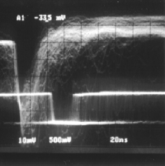
Figure 7: Chamber signal at the entrance of the comparator and the shaped signal.

The $3~{}\mathrm{m}$ long sense wires are very efficient antennas and collect easily radio emitters and noise. The drift cell field shaping strips provide already a good shielding which has been reinforced by a complete shielding of the chamber with a $12~{}\mathrm{\mu m}$ thick aluminium foil. Tests have shown that thicker shielding does not improve the situation. The chamber is essentially composed of insulating material. It is therefore necessary to define properly ground references. For this purpose, the amplifiers have been mounted on a board whose ground support covers the entire board. On the side of the chamber panels, $3~{}\mathrm{mm}$ thick copper bars have been implanted and the ground plane of each electronic board is connected to them. We found experimentally that the strips in front of the sense wires had to be connected directly to the electronic ground of the board. Although the strip was already connected to ground through the voltage divider, this operation reduces the radio and noise background by more than one order of magnitude.

3.2 The TDC’s

The signals from the discriminators are encoded by modified LeCroy multi-hit TDCs 1876 [12] operated in a “common stop” mode. The TDCs hold in memory at most the last 16 hits for each channel over a time period of $\rm 64~{}\mu s$.

To encode the signal on sixteen bits ($\rm 1~{}ns$ lsb corresponding approximately to $\rm 50~{}\mu m$ drift distance), these TDCs :

1. record the arrival time $t_{start}$ of the “hits”, i.e. pulses from the drift chamber comparators. A counter performs a fourteen bit coarse measurement at twice the board clock frequency ($125\,\mathrm{MHz}$). Three delay lines give an additional 2 bit resolution.

2. record the arrival time $t_{stop}$ of the stop signal, i.e. the pulse from the experimental trigger, delayed to encompass the maximum drift time.

3. store the difference $t_{stop}-t_{start}$ for each valid hit. Thus, small TDC values correspond to large drift times.

The counter structure guarantees that the integral non-linearity of the encoded time difference depends only on the main clock oscillator stability. The differential non-linearity on the individual input signals is induced by the internal delay lines and the clock interleaving. Each board and channel was individually qualified in the lab using a digital delay as reference [14]. The integral non linearity was found to be negligible. The overall error on each channel was smaller than $800\,\mathrm{ps}$.

The TDCs were modified to store all converted informations from successive events in internal buffers during the neutrino spills ($4~{}\mathrm{ms}$), so the dead-time is limited to the time needed to handle the Common Stop ($1~{}\mathrm{\mu s}$) and to transfer the data from the encoding chip to the buffer ($150~{}\mathrm{ns}$ per hit). Thus the dead time $T_{D}$ induced by the readout of the drift chambers can be expressed as :

$$T_{D}=1\,\mathrm{\mu s}+150\,\mathrm{ns}*maximum\,\#hits\,per\,module\,per\,event$$

To reduce the dead time and to insure that no buffer overflow occurs, the signals from a given chamber were distributed across different TDC modules. The minimal time between successive hits was found to be $9.5~{}\mathrm{ns}$ with a standard deviation of $0.9~{}\mathrm{ns}$ across all TDCs. Extremum values were $5~{}\mathrm{ns}$ and $20~{}\mathrm{ns}$.

4 The drift chamber construction

The goal was to build more than 50 chambers within one and a half year. The production line was split into 6 main phases with 6 corresponding main shops:

• panel drilling

• strip positioning and gluing

• frame and printed circuit board gluing

• strip connections

• wire positioning and soldering

• electric tests and assembly

Each phase had to be carried out within 5 days and was operated by two technicians. A chamber needed about 5 weeks to be built. Finally the chamber was tested with cosmic particles.

4.1 Panel selection and drilling

After sand-papering and a visual control of the state of the surfaces, concavity and thickness were taken into account to select the panels.

In more than 200 panels, 19 holes had to be drilled: 4 in order to assemble the chamber and for precise positioning measurements, 9 for the spacers and 6 to build a module (as described in subsection 2.3). A $\rm 9~{}m^{2}$ gauge built with the same materials as the panels (aramid honeycomb + kevlar epoxy skins) was used. On this gauge metallic inserts supported drilling barrels.

4.2 Strip gluing

The straightness of the strip bands was checked before gluing them on the panels with a bi-component polyurethane glue. The glue toxicity led us to build a special closed area around the stripping shop with fast air replacement. The operators had to wear breathing masks and appropriate gloves. To glue with precision the strips on the panels, we used a table with a frame allowing precise relative indexing between the panels and the strip laying tool developed by our CERN collaborators. After gluing each band of 144 strips (5 bands per panel), a measurement of the strip positions was performed with a position gauge attached to the frame and parallel to the strips. In case of bad positioning, it was possible to quickly remove the band from the panel. After gluing of the 5 bands, a strip position measurement with respect to the reference holes was performed again.

4.3 Frames and printed circuit boards

A week later, gas tight frames as well as printed boards for high voltage and signal connections were glued on the strips and the panels (see figure 3) using epoxy glue.

4.4 Strip connections

Before connecting the strips to the flexible high voltage bus, an electric test was performed to find short-circuits between strips. An automatic pneumatic stapler was used to establish 4000 connections per chamber. Thereafter, the 3 wire supporting epoxy-glass rods were glued perpendicularly over the strips to reduce the gravitational and electrostatic sagitta of the wires. Finally, another electric test was performed to check the continuity and insulation of the connected strips and the bus.

4.5 Wire positioning and soldering

Using a position gauge, reference lines for wire positioning were engraved on the printed circuits at the two ends of the chambers. Then the wires were brought into alignment with engraved lines using a video camera equipped with a zoom. The tensions were adjusted to $\rm 50~{}$g for the sense wires (just below the limit of elastic deformation) and $\rm 200~{}g$ for the field wires. After soldering and gluing the wires on printed circuits at both ends, tensions were checked by a resonance frequency measurement. After possible replacement of some wires showing bad tension, all wires were glued on the 3 perpendicular epoxy-glass rods. Then the position of 10 sense wires with respect to the 4 pins used to close the chamber (one at each corner of the chamber) were measured using an optical ruler. These measurements were used later on as a starting point for the global geometrical alignment.

4.6 Electric test and assembly

We checked that the test lines running on the chamber side induced signals on all the sense wires by capacitive coupling (see figure 3). Then some electrical tests were performed on each plane.

First, the insulation resistance between the strips was measured. Then a negative high voltage ($\rm-7000~{}V$) was applied to the strips and to the field wires. Measurements were performed on the field wires in order to check the leakage current. In case of a large leakage current cleaning of the board was necessary. After decreasing the HV to $\rm-3200~{}V$ (the nominal value) positive high voltage was applied to the sense wires to check the leakage current. Then during about 2 hours, a sense wire cleaning was performed by applying a negative high voltage on the sense wires and no voltage on the strips and field wires. We observed a current decreasing with time on the sense wires. When no more current variation was detected we stopped the cleaning process. After these tests, the chamber was assembled. The planes were glued together with a silicon joint laid down along the gas tight frames. After closing a gap, the same electrical tests were done before closing the next one. Once the three gaps were closed, the nine insulated screws corresponding to the nine spacers and the gas connectors were put into place. Three days later, the chamber was filled with argon in order to verify the gas tightness.

4.7 Cosmic test

Before being sent to CERN for the final installation in the experimental area, each chamber was tested with cosmic rays [15]. The experimental setup is shown in figure 8. The chamber was completely equipped with preamplifiers and filled with $\rm Ar(40\%)-C_{2}H_{6}(60\%)$ gas mixture at atmospheric pressure. A first data taking was done by sending signals on the test lines with a pulser to check that the electronic chain (preamplifiers, cables, TDC) was functioning correctly. Then data taking with cosmic particles was performed. The coincidence of three scintillation counters, $\rm 3~{}m$ long and $\rm 30~{}cm$ wide, defined the crossing of a particle through the chamber. The drift times and the number of hits on each wire were recorded. With the signal hit map it was possible to identify some potential problems: noisy wires, dead wires, efficiency losses, etc. We had to open some chambers to replace bad wires. Drift time distributions could show some possible problems related to strip band positioning. Figure 9 shows a non uniform drift time distribution observed with a bad strip band positioning following a mistake made during the gluing of the strips as compared to a normal drift time distribution. The chamber was dismounted and new strip bands were glued on the panel.

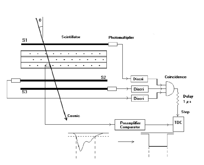
Figure 8: The cosmic test setup.

Figure 9: Drift time distribution as measured by the cosmic test setup. Top: for correctly aligned strip bands. Bottom: for misaligned ones.

5 Gas system and slow control

In order to ensure a stable operation of the drift chambers during long periods of time, a large number of parameters have to be kept under control, such as the quality of the gas mixture, high and low voltages, temperature, pressure, etc. A dedicated slow control system has been developed to monitor these parameters and raise alarms when necessary.

It was decided to use a common gas system for the target drift chambers and the muon chambers of the NOMAD experiment. The latter were muon chambers recycled from the UA1 experiment [16], with a total volume of 40 m³ compared to 10 m³ for the target drift chambers, and both systems used a 40% argon - 60% ethane gas mixture. Such a mixture exhibits a large plateau in drift velocity as a function of the ratio of electric field over pressure, so that the effect of atmospheric pressure variations is minimized. The common input gas flow, whose composition was monitored every 10 mn, was split between the two subsystems. The gas was then distributed to each drift chamber, individual flows being adjusted using a manual valve. Cheap quarter turn valves were used and showed a good stability during the 4 years of operation. A flowmeter on each chamber with digital reading (AWM3300 by Honeywell) allowed to perform the initial setup or subsequent adjustments of the valves. Another flowmeter on the return circuit of each chamber allowed to determine the output flow. All these flowmeters had previously been individually calibrated both for the standard argon-ethane mixture and for pure argon. The flowmeters were interfaced with a MacIntosh running Labview [17] for a permanent monitoring of individual input and output gas flows.
Any significant departure from reference values for input or output flows of individual chambers generated an alarm in the control room of the experiment. The typical input flow for each chamber was set around 25 liters/hour (the gas volume is 200 liters per chamber). The typical leak rate was about 5 liters/hour. Some chambers had leaks up to 12 liters/hour (in which case the input flow was increased to 30 liters/hour). Such high leak rates are inherent to the conception of these chambers (due to the porosity of the panels), but no loss in efficiency was observed for the chambers with higher leak rates. The oxygen content in the output gas mixture was about 500 ppm in the global return circuit of all drift chambers and was continuously monitored to insure that there was no loss in efficiency. A strong ventilation of the internal volume of the magnet ensured that no accumulation of gas from the chambers could occur (safety gas detectors were installed in this volume). To avoid accidental overpressure, each chamber was protected by bubblers, set up in parallel both on input and output circuits. The gas flow through the drift chambers was assisted by an aspirator pump. The gas from the return circuit was partly recycled after going through oxygen and water traps, in order to save on ethane consumption.

The monitoring program was also controlling the correct value of the low voltages for the electronics of the chambers, including discriminator thresholds and the setting of the $B/\bar{B}$ switch for strip high voltages (corresponding to the magnetic field being on or off, see subsection 2.5); it also controlled the values of the high voltages (through a CAMAC interface to the CAEN power supply), for cathodes and anode wires. In particular, automatic tripoffs of wire planes due to transitory overcurrents generated an alarm in the control room.
Such trips occured on a very small number of planes for which the electrostatic insulation had some weaknesses, very difficult to localize as the overcurrent appeared after several hours or days of perfect operating conditions. Only 2 such planes out of 147 had to be permanently switched off towards the end of the data taking.

The quality of the alignment (subsection 6.1) for the chambers was checked daily with a sample of 10,000 muons, and a complete realignment was done when a wider residual distribution was observed. Typically each yearly run was divided in 5 to 10 periods with different alignment parameters. This was found sufficient to adequately take care of slow changes in the gas composition as well as of significant variations of the atmospheric pressure during some periods.

6 The drift chamber performances

The chambers are operated at 100 V above the beginning of the efficiency plateau, which was found to be 200 V wide. Under these conditions, the typical wire efficiency is 0.97, most of the loss being due to the wire supporting rods. The TDC’s measure a time difference with a common stop technique:

$$\Delta t=t_{stop}-t_{start},$$

where

$$t_{start}=t_{interaction}+\Delta t_{tof}+\Delta t_{drift}+\Delta t_{wire}+\Delta t_{elect}$$

which takes into account the interaction time ($t_{interaction}$), the time of flight of the measured particle between the interaction point and the measurement plane ($\Delta t_{tof}$), the drift time of electrons ($\Delta t_{drift}$), the signal propagation time along the sense wire ($\Delta t_{wire}$) and the signal propagation time in the electronic circuits ($\Delta t_{elect}$).

$$t_{stop}=t_{interaction}+\Delta t_{tof\_trig}+\Delta t_{delay}$$

consists of the time of flight of the triggering particle ($\Delta t_{tof\_trig}$) and a delay ($\Delta t_{delay}$) long enough that the stop signal arrives after all possible start signals. $\Delta t_{delay}$ is of the order of one microsecond. The time measured by a TDC is then

$$\Delta t=(\Delta t_{tof\_trig}+\Delta t_{delay})-(\Delta t_{tof}+\Delta t_{drift}+\Delta t_{wire}+\Delta t_{elect})$$

This time can be corrected for $\Delta t_{delay}$ (see subsection 3.2), $\Delta t_{elect}$ and $\Delta t_{wire}$ (as soon as the $x$ coordinate of the hit along the wire is known), so that the true drift time is extracted.

The coordinate $c$ is obtained from the coordinate $c_{w}$ of the wire and from the drift distance $d$, which is a function of both the drift time $\Delta t_{drift}$ and the local angle $\phi$ of the track in the plane perpendicular to the wires. The drift distance is either added to or subtracted from $c_{w}$. This is known as the up-down ambiguity:

$$c=c_{w}\pm d(\Delta t_{drift},\phi)$$

and this ambiguity is only resolved at the level of track reconstruction and fit.

6.1 Spatial resolution

The spatial resolution depends on the precise knowledge of the wire positions and of the time-to-distance relation. Since the wires are glued at both ends and on 3 vertical rods as mentioned in subsection 2.5, the wire shape is approximated by 4 segments joining these points. The vertical positions of these 5 points for each of the 6174 wires have then to be precisely determined.

One time-to-distance relation is defined for each plane independently, as different planes could work under different gas and high voltage conditions. The precise determination of the drift velocity is important because a mistake of one percent leads to a bias in the spatial resolution of the order of several hundred microns ($d_{max}\cdot\frac{\Delta V_{drift}}{V_{drift}}={3.2\ \rm{cm}}\cdot 0.01=320\ \mu$m).

A special alignment procedure [18] was set up to measure wire positions and shapes, time-to-distance relationship and other relevant quantities using muons crossing the NOMAD detector.

Track reconstruction details are given in the next section. Our alignment procedure is based on the residual distributions of reconstructed tracks (a residual is the difference between the hit coordinate and the reconstructed track coordinate at a given measurement plane). Initial wire positions are first taken from the geometers’ survey and the mechanical measurements, and then corrected to minimize any systematic offset in an iterative way: typically 3 to 5 iterations on 100,000 muons samples are needed for the procedure to converge.

The procedure then focuses on the time-to-distance relation. A model used to describe the main time-to-distance relation is shown schematically in figure 10: ionization electrons first drift parallel to the strip plane with velocity $V_{1}$ and then radially to the wire with velocity $V_{2}$. For each plane these 2 velocities are extracted again by minimizing offsets in signed residual distributions. The dispersion of $V_{1}$ values measured for different planes was found to be 1.7%.

Figure 10: A model used to describe the drift of electrons in the drift cell.

The $z$ positions of the measurement planes are also updated during this global alignment procedure.

Figure 11: Residuals for a sample of normal incidence tracks similar to the ones used for the alignment of the drift chambers.

Figure 12: The dependence of the track residuals on the drift distance for different crossing angles.

At the end of this procedure (typically 10-15 iterations over samples of 100,000 muons) the distribution of the residuals for tracks perpendicular to the chambers is shown in figure 11. This distribution has a $\sigma$ of about 150 $\mu$m (for normal incidence tracks) and confirms the good spatial resolution of the NOMAD drift chambers. The spatial resolution averages to 200 $\mu$m for tracks originating from neutrino interactions (the average opening angle is 7 degrees). The dependence of the resolution on the drift distance and the crossing angle $\phi$ is shown in figure 12. At small drift distances, the angular dependence is essential due to the electronic threshold (see subsection 3.1). At large drift distances, because of the non-uniformity of the electric field near the strips, the angular effect is enhanced.

6.2 Efficiency

The drift chamber efficiency and its dependence on the track angle and track position in the drift cell were carefully studied using muons crossing the detector between two neutrino spills.

The inefficiency was computed as a function of the $x$-coordinate (along the wire). The results are given in figure 13. This distribution can be well fitted by a constant ($\approx 2.4\%$) and three gaussian functions with a width of $\approx 6$ mm centered at the supporting rod positions. As a result, the efficiency in the region between supporting rods is $\varepsilon_{min}\approx 97.6\%$ consistent with our expectations and we confirm that the inefficiency is caused mainly by the presence of the rods.

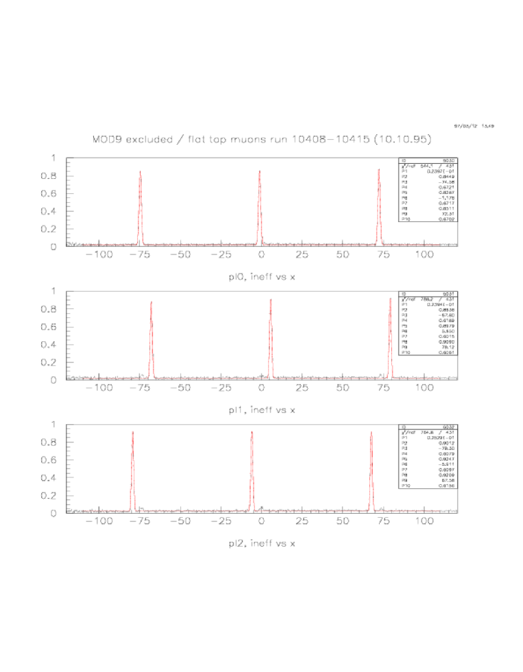
Figure 13: The inefficiency (1-$\varepsilon_{min}$) as a function of the $x$-coordinate (along the wire). Peaks correspond to the wire supporting rods. The small bumps in the second (pl1) and third (pl2) planes are due to spacers used as chamber supports.

Further studies show that the major efficiency loss is not due to the absence of the hit in a measurement plane but due to the non-Gaussian tails in the residual distributions. If one extends the road for the hit collection during the track reconstruction a maximal drift chamber efficiency of $\varepsilon_{max}\approx 99.7\%$ can be obtained. One can also study the efficiency as a function of the track position in the drift cell (figure 14): the main loss occurs at the edge of the cell where the drift field is less uniform (see figure 5) .

Figure 14: The dependence of the hit finding efficiency on the track position in the drift cell.

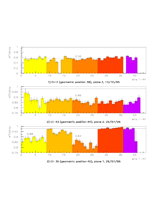
Figure 15: Examples of hardware efficiency losses for some pathological drift chamber planes. The horizontal solid line shows an efficiency $\varepsilon=0.98$ for normal chambers. The different shaded areas indicate different strip bands. (1) for planes with short circuits between strips: the efficiency loss is $\approx 42\%$; (2) for disconnected field wires: the efficiency loss is $\approx 12\%$; (3) for misaligned strip bands: the efficiency loss is $\approx 10\div 15\%$.

There are other hardware effects which cause efficiency losses: planes with short circuits between strips, disconnected field wires, misalignment of a wire with respect to the facing strip band. These effects have been studied in details (see figure 15 for a particular example) and the following typical values have been obtained:
- planes with short circuits between strips: efficiency loss $\approx 40\%$,
- disconnected field wires: efficiency loss $\approx 10\%$,
- misaligned strip bands: efficiency loss $\approx 10\div 15\%$.

We did not notice any correlation of the loss in efficiency with oxygen contamination in the gas mixture or chamber leak rate.

As an example, the overall hardware performance of the NOMAD drift chambers during the 1996 run data taking period was the following: among 147 planes, 1 to 2 planes were switched off due to unrecoverable problems (such as a broken wire), 2 to 3 planes suffered from short circuits between strips and 3 planes had disconnected field wires.

6.3 Afterpulses

The problem of afterpulses (or bounces) was present in the drift chambers response: some of the hits can be accompanied by one or several other hits on the same wire. The time difference between the hit included in a given track and the other hit on the same wire is shown in the distribution of figure 16. We have noticed two contributions: the first one is symmetric in time and the second one is concentrated at about 50 ns after the first digitization. The former contribution was attributed to the emission of low-energy $\delta$-rays which produce random hits in the drift cell crossed by the track, while the latter contribution was associated with the smearing of the electron cloud consisting of several clusters which could trigger another digitization after the arrival of the first electron.

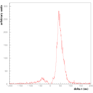
Figure 16: Example of the time difference (in ns) between a second hit on the same wire and the hit included in a given track.

It was found that the rate of afterpulses depends on the track angle and track position in the drift cell. These afterpulses were included in the simulation program.

The knowledge gained by the studies of resolution, efficiency and the presence of afterpulses was used during the track reconstruction in the drift chambers. The dependence of the resolution on the drift distance and track angle was parametrized and implemented at the level of track search and fit. A special bounce filter was developed to cope with the presence of afterpulses for the hit selection.

7 The drift chamber reconstruction software

In the NOMAD experiment trajectories of charged particles are reconstructed from the coordinate measurements provided by the drift chamber (DC) system. The main purpose of the drift chamber reconstruction program is to determine the event topology and to measure the momenta of charged particles. The reconstruction program for the NOMAD drift chambers is extremely important for the performance and sensitivity of the experiment. A very high efficiency of the track reconstruction is required in order to provide good measurement of event kinematics for the oscillation search. We have also to be sure that the measured track parameters do not deviate significantly from the true particle momenta, i.e. the reconstruction program should provide good momentum resolution. The amount of ghost tracks should be minimized. Since in the NOMAD setup the amount of matter crossed by a particle between two measurement planes cannot be neglected, the effects of energy losses and multiple scattering must be carefully taken into account.

The task of the reconstruction program is two-fold. First, it should perform pattern recognition (track search), namely to decide which individual measurements provided by the detector should be associated together to form an object representing a particle trajectory. At the next stage, a fitting procedure should be applied to this set of measurements in order to extract the parameters describing the trajectory out of which the physical quantities can be computed.

The track finding procedure consists of two loosely coupled tasks: the first one guesses possible tracks from hit combinatorics, and provides initial track parameters. The second task attempts to build a track from the given parameters by repeatedly collecting hits, fitting and rejecting possible outliers. The track is claimed to be fitted when no more hits can be added to it. We developed several approaches to the first task which are summarized in [19]. A short overview is given here.

7.1 Searching for candidate tracks

7.1.1 The DC standalone pattern recognition

The algorithm presented here does not make use of any prior information for the track search: the parameter space has 5 dimensions (or even 6 if one adds the trigger time jitter). The combinatorics from hits to likely track parameters goes in two steps: we first associate hits from the 3 planes of the same chamber in triplets, which provide some 3-dimensional (3D) information; we then search combinations of 3 triplets belonging to the same helix.

DC Triplets
A drift chamber is made of 3 sensitive planes measuring the U, Y and V coordinates, where:

$u\;=\;y\cdot\cos 5^{\circ}\;-\;x\cdot\sin 5^{\circ}$ and $v\;=\;y\cdot\cos 5^{\circ}\;+\;x\cdot\sin 5^{\circ}$

Four parameters define locally the track (across one chamber, one can neglect its curvature): we use 2 coordinates in the central Y plane $x,y$ and 2 slopes $\alpha_{x}$, $\alpha_{y}$ (with respect to Z). From 3 hits in the 3 planes and 3 chosen signs (we decide if the track crossed above or below each involved sense wire), we have 3 measured coordinates U, Y and V. With 3 measurements, we cannot estimate the 4 local parameters. The measured combinations are:

$$y = Y$$

$$2\Delta z\ \alpha_{x}\sin 5^{\circ} = U\;+\;V\;-\;2Y\cos 5^{\circ}$$

$$x+\Delta z\ \ cotg5^{\circ}\ \alpha_{y} = (V-U)/(2\sin 5^{\circ})$$

where $\Delta z$ is the distance between two consecutive measurement planes (about 2.5 cm). The second equation can be turned into a constraint by assuming that $\alpha_{x}$ does not exceed a certain bound (e.g. $|\alpha_{x}|<1$). Since $\sin 5^{\circ}\simeq 0.087$, this constraint becomes the first tool to assemble triplets. The third equation shows that $x$ remains poorly known as long as the $y$-slope ($\alpha_{y}$) of the track is unknown: changing $\alpha_{y}$ by 1 shifts $x$ by about 30 cm.

To build triplets, we compute $\Delta=U\;+\;V\;-\;2Y\cos 5^{\circ}$ for all hits and sign combinations inside a chamber, and solve ambiguities by keeping no more than 2 triplets per signed hit, possible triplets being ranked by increasing $|\Delta|$.

Helix search
Triplets are used to initiate the track search. With 3 triplets we are able to test whether they belong to the same trajectory. At this step, we still ignore the magnetic field variations and check the 3 triplet combinations against a perfect helix. From the 3 $y$ positions, we compute 3 slopes in the YZ plane which enable to compute 3 $x$ coordinates from the third equation above. We can then reliably compute drift distances, including a sensible time correction due to the signal propagation along the sense wire and using the known track slope for the time-to-distance relation (see subsection 6.1). We then recalculate the 3 triplet ($x,y$) positions from these precise drift distances and slopes.

The most sensitive criterion is to check by how much the $x$ coordinates depart from the same helix. Calling $\phi$ the angle with respect to (e.g) horizontal in the YZ plane, the residual is:

$x^{extrap}-x_{2}=x_{1}+(\phi_{1}-\phi_{2})\cdot\frac{x_{3}-x_{1}}{\phi_{3}-\phi_{1}}-x_{2}$

where the subscript refers to the triplet number. For accepted combinations, we compute the track parameters at the central triplet position and feed it to the track construction task.

7.1.2 The coupled TRD and DC track search

The TRD detector [6] is located downstream of the target and has a total length of 1.5 m in Z. Five drift chambers are interleaved in the TRD modules, which measure the $x$ coordinate of tracks by means of vertical cylindrical xenon filled straws, 1.6 cm in diameter without drift time information. These additional drift chambers allow to improve the momentum resolution for reconstructed tracks and provide more precise track extrapolation to the preshower and electromagnetic calorimeter front face.

The first step of the coupled TRD-DC track search algorithm [19] consists in reconstructing TRD tracks (in XZ projection) using the 9 planes of straws. The coarse spatial sampling enables to ignore the effects of curvature in the XZ plane: a TRD track defines a position and a slope in the XZ plane. These TRD tracks can only be used in the most downstream part of the target, and this TRD seeded track search only applies to the 10 most downstream drift chambers. In those chambers, and for every TRD track, we can build triplets using the $x$ and $\alpha_{x}$ values, thus triplets are now constrained. We can even build doublets, a combination of two hits in a given chamber. The helix search can then be carried out in the same way as for the DC standalone case. In a later version, we slightly improved the reconstruction quality of complicated events by searching circles among DC hits projected on a vertical plane containing the TRD track. This was made possible by the increase of CPU power of low cost computers.

7.1.3 Track search using vertex information.

Advanced track construction algorithms which take into account the information about reconstructed vertices have also been developed [20].

Tracks from 1 vertex
Searching a track that emerges from a vertex reduces the parameter space dimension by 2 units. Since the vertex is already a 3D point (much better defined than any triplet), we can find a short track which only has 2 triplets. The triplets are here searched for with $x$, $\alpha_{x}$, $y$ and $\alpha_{y}$ loosely constrained to point back to the vertex at hand. This enables to find tracks at large angles with respect to the beam direction. Having constructed these triplets, the triplet combinatorics for helix search can be run in the same way as described previously. The vertex is considered as a triplet for which the $x$ position does not depend on the YZ slope. The new track is only accepted if it enters the seed vertex with an acceptable $\chi^{2}$ increase.

Tracks joining 2 vertices
Hadron interactions may be reconstructed as secondary vertices or hanging secondary tracks without the primary hadron being found. We designed a track search algorithm to find tracks either between 2 actual vertices (i.e. vertices with at least 2 attached tracks) or between an actual vertex and a starting point of a standalone track (in which case its actual vertex may slide along the track direction). This is a track search with 1 or 2 free track parameters which does not go through triplets.

7.2 Building tracks

This task uses track parameters (given by the previous track search) at any given plane as a seed and tries to build a track.

The first step consists in collecting hits upwards and backwards from a given plane within a road (typically 3 mm). The hit search makes use of all available information by computing drift distances corrected for slope and $x$ position. The track global time offset with respect to the trigger time is still unknown and its average value is taken first. Later on, the time offset of the highest momentum track already found is used for all the tracks in the event. The collection stops when too many measurement planes are crossed without a matching hit or when several hits are found within a control road in the same plane. Missing hits can be “excused” if the wire or plane at the expected position is dead, or if a hit with a smaller drift time on the wire may hide the expected digitization. A track may go to the next step if it has enough hits, and a high enough average efficiency. At this last step, we first fit the hit list. The candidate track disappears if the fit diverges or if the $\chi^{2}$ is too high. We then discard hits that exhibit a too high $\chi^{2}$ contribution (the cut is usually 10). From now on, the track gets re-fitted whenever we add one hit, and the $\chi^{2}$ increment decides whether a hit may enter a track. Using the Kalman filter technique makes this approach acceptable in terms of CPU. We then try to collect hits in planes crossed by the track but where hits are originally missing. We finally collect hits downstream and upstream, and iterate collection over the track, downstream and upstream until the track hit list stops evolving. We store the track in the track repository, and mark its hits as no longer available for triplet construction or hit collection by other tracks. They however still remain examined for the hit “excuse” mechanism.

7.3 Track model

The track model describes first the dependence of the measurements on the initial values in the ideal case of no measurement errors and of deterministic interactions of a particle with matter. During its flight through the detector a particle however encounters various influences coming from the materials of which the detector is built. There are effects which can be taken into account in a deterministic way: average energy loss and average multiple scattering. They depend in general on the mass of the particle, its momentum, the thickness and nature of the traversed material. The detailed information on the track model used for the track reconstruction in the NOMAD drift chamber system can be found in [21].

The track model has been used to develop an extrapolator package which is heavily used for the track construction and fit [21]: there, a precise track model and a good magnetic field description are important to ascertain that the fitting procedure is unbiased. The magnetic field inside the magnet has been carefully measured and parameterized. In the detector fiducial volume the main component of the field $B_{x}$ has been found to vary within 3%. Uncertainties in the track model predictions due to small non-zero values of the two other components ($B_{y}$ and $B_{z}$) are negligible compared to the effect of multiple scattering. This allows to use only the local value of the main field component $B_{x}$ for the track model calculations [22].

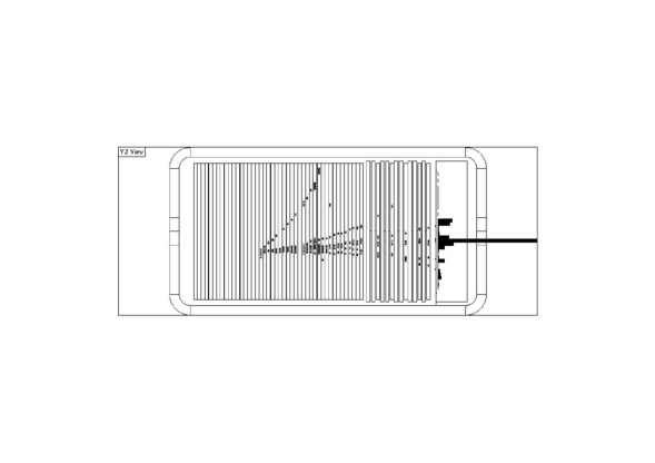
Figure 17: Raw hits before the reconstruction in a real data event. One can easily see a dead drift chamber plane in the middle of the detector.

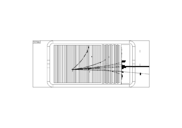
Figure 18: The same event as on figure 17 after performing DC reconstruction and particle identification.

7.4 Track fit

After pattern recognition, one has to determine the track parameters, in particular charged particle momenta. The Kalman filter technique [23, 24] is adapted to fulfill this task. Some details on the implementation of the Kalman filter for the NOMAD drift chambers can be found in [22].

The track fit proceeds in 3 steps: forward filtering, backward filtering and smoothing [23]. The smoothing provides the best possible track position estimate at any measurement location, thus allowing to efficiently remove wrong associations.

The fitting routine performs those 3 steps until the $\chi^{2}$ modification between 2 fits is below a typical value of 0.1.

The Kalman filter technique was implemented in two different ways: using weight and covariance matrices. The latter was found faster since it allows to avoid several matrix inversions per hit when the effect of multiple scattering is taken into account.

A raw event from real data can be seen in the figure 17. The result of DC reconstruction and particle identification is shown in figure 18.

An algorithm developed on the basis of the Kalman filter technique to search for potential break points corresponding to hard bremsstrahlung photons emission is discussed in [22].

7.5 Vertex reconstruction

7.5.1 Vertex finding and fitting

The vertex reconstruction is performed with reconstructed tracks. The major tasks of the vertex package are:

• to determine the event topology (deciding upon which tracks should belong to which vertex);

• to perform a fit in order to determine the position of the vertex and the parameters of each track at the vertex;

• to recognize the type of a given vertex (primary, secondary, $V^{0}$, etc.).

The vertex search algorithm proceeds as follows. For both ends of each track one calculates the minimal weighted distances to all the other tracks. Then one takes the point corresponding to the minimal distance as a starting vertex position; tracks close enough to the chosen point are added to the list of tracks of the candidate vertex. A fit algorithm (Kalman filter) is applied next to reject unmatching tracks. Finally, one defines the topology of the reconstructed vertex assuming the direction of the incoming particle and the balance of momenta between tracks belonging to this vertex: e.g., a track connected by its end to a vertex could be either a parent track (scattering vertex or decay of a charged particle) or a track going backwards (in that case it has to be reversed, i.e. refitted taking into account energy losses in the right way). Additional vertices are searched for and reconstructed starting from unused track ends. The Kalman filter technique is used to allow fast vertex fit and provides a simple way to add or remove tracks from an existing vertex without completely refitting it.

7.5.2 Vertex position resolution

Most neutrino interactions in the active target occur in the passive panels of the drift chambers. Figure 19 shows the distribution of primary vertices in a plane perpendicular to the beam. A fiducial cut of $-120\leq~{}{x,y}~{}\leq 120$ cm is imposed. The gradual decrease of the beam intensity with radius can be easily seen. The 9 dark spots of high intensity are caused by the spacers which are inserted in the chambers in order to increase their rigidity and maintain the gap width (see subsection 2.3).

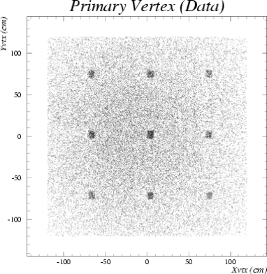
Figure 19: The positions of reconstructed neutrino interaction vertices from experimental data in a plane perpendicular to the beam direction; see text for details.

Figure 20 shows the distribution of primary vertices along the beam direction. The information from all drift chambers has been folded to cover the region of $\sim$10 cm around the centre of each chamber. One can easily see that the bulk of neutrino interactions occurs in the walls of the drift chambers. The eight spikes in this distribution correspond to the kevlar skins of the drift chambers (see figure 2). Regions in $z$ with a smaller number of reconstructed vertices correspond to the honeycomb panels and the three gas-filled drift gaps.

Figure 20: The positions of reconstructed neutrino interaction vertices in the experimental data as measured along the beam direction; see text for details.

The vertex position resolution was checked using MC simulation. The results are presented in figure 21. Resolutions of 600 $\mu$m, 90 $\mu$m and 860 $\mu$m in $x$, $y$ and $z$ respectively are achieved.

Figure 21: The vertex position resolution for reconstructed $\nu_{\mu}$ CC MC events. The resolution is 600 $\mu$m, 90 $\mu$m and 860 $\mu$m for $x$, $y$ and $z$ respectively.

7.6 Implementation

The drift chamber reconstruction is a software package written in C language in an object oriented way. It includes track and vertex search and fit, track extrapolation package and a graphical display which was found very useful to check the performances of the pattern recognition algorithms and to study possible improvements.

7.7 CPU considerations

The overall CPU time needed for the event reconstruction in the drift chambers strongly depends on the complexity of the event. Events with more than 1000 hits are not reconstructed. Genuine neutrino interactions are reconstructed in about 10 s on a PC at 300 MHz. Half of the time is spent in combinatorics, the other half in the extrapolation of candidate track parameters (and of the error matrix when needed) which is necessary when collecting hits and fitting tracks.

The reconstruction algorithms have been explicitely optimized to reduce the CPU time required. However, this optimization became less critical with a very fast increasing performance of low cost computers along the duration of the experiment.

8 Check of the drift chamber performances using experimental data

It was important to validate the claimed performances of the drift chambers using experimental data.

8.1 Momentum resolution

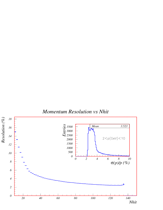
Figure 22: Average momentum resolution as a function of the track length (number of hits in the fiducial volume of drift chambers). The insert shows the distribution of the number of tracks at a given resolution.

The momentum resolution provided by the drift chambers is a function of momentum and track length. For charged hadrons and muons travelling normal to the plane of the chambers, it can be approximated by

$$\frac{\sigma_{p}}{p}\approx\frac{0.05}{\sqrt{L}}\oplus\frac{0.008\times p}{\sqrt{L^{5}}}$$

where the momentum $p$ is in GeV/c and the track length $L$ in m. The first term is the contribution from multiple scattering and the second term comes from the single hit resolution of the chambers. For a momentum of 10 GeV/c, the multiple scattering contribution is the larger one as soon as the track length is longer than 1.3 m.

Figure 22 shows the resolution as a function of the number of hits (related to the track length) as obtained from a fit of real tracks. A momentum resolution of $3.5\%$ in the momentum range of interest ($\rm 2<p(GeV/c)<10$) is achieved.

For electrons, the tracking is more difficult because they radiate photons via the bremsstrahlung process when crossing the tracking system. This results sometimes in a drastically changing curvature. In this case, the momentum resolution as measured in the drift chambers is worse and the electron energy is measured by combining information from the drift chambers and the electromagnetic calorimeter [7, 21].

8.2 Neutral strange particles

A study of neutral strange particles can provide some information related to the performance of the drift chambers.

A decay of a neutral strange particle appears in the detector as a $V^{0}$-like vertex: two tracks of opposite charge emerging from a common vertex separated from the primary neutrino interaction vertex [18, 25, 26]. Figure 23 shows an example of a reconstructed data event with two such $V^{0}$’s.

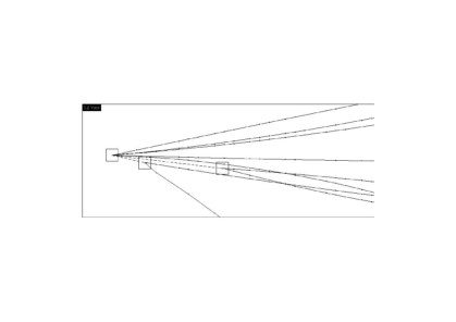
Figure 23: A reconstructed data event (zoom on the primary vertex) containing 2 $V^{0}$ vertices identified as $\rm\Lambda$ and $\rm\overline{\Lambda}$ decays. The scale on this plot is given by the size of the vertex boxes ($3\times 3$ cm²).

The quality of the reconstruction in the NOMAD drift chambers allows a precise determination of the $V^{0}$ decay kinematics as can be seen on the so-called Armenteros’ plot (figure 24). This figure is obtained by plotting for each neutral decay the internal transverse momentum ($P_{t}^{+}$) versus $\rm\alpha$, the asymmetry of the longitudinal momenta of the two outgoing tracks ($\alpha=\frac{P_{l}^{+}-P_{l}^{-}}{P_{l}^{+}+P_{l}^{-}}$). Without any cut, each type of neutral strange particle appears clearly on the figure.

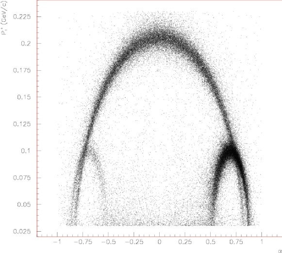
Figure 24: Armenteros’ plot for reconstructed $V^{0}$’s: $\rm K^{0}_{s}$’s cluster on the large central ellipse, $\rm\Lambda$’s on the small right ellipse and the smaller sample of $\rm\overline{\Lambda}$’s on the left one.

$V^{0}$’s allow to check the quality of the drift chamber reconstruction by computing invariant masses corresponding to different neutral strange particle hypotheses ($\rm K^{0}_{s}$, $\rm\Lambda$, $\rm\overline{\Lambda}$):

$$M^{2}=M^{2}_{+}+M^{2}_{-}+2(E^{+}E^{-}-P^{+}P^{-}\cos\theta)$$

where $M_{+}$ and $M_{-}$ are the masses of positive and negative outgoing particles, $E^{+}$ and $E^{-}$ are their energies and $\theta$ is the angle between them. Figure 25 shows $\rm K^{0}_{s}$ and $\rm\Lambda$ normalized invariant mass distributions for both data and Monte Carlo. The widths of these distributions are related to the momentum resolution and are in good agreement with what is expected from figure 22.

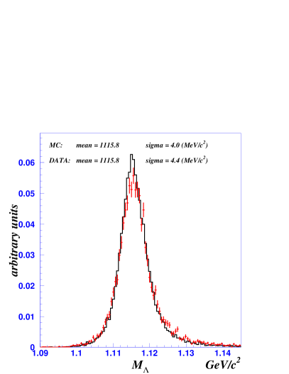
Figure 25: Invariant mass distributions for identified $\rm K^{0}_{s}$’s  (left) and $\rm\Lambda$’s (right).

8.3 Test of the global alignment of the drift chambers

The alignment procedure described in section 6 may lead to a systematic displacement of the calculated wire positions with respect to the real positions, so that a straight track would appear to be slightly curved. This would obviously bias the momentum measurement. We show now how we used $V_{0}$ decays to measure such a bias and eventually correct for it.

If we call the curvature bias $\varepsilon$ ($\varepsilon=<1/p_{rec}-1/p_{true}>$), its influence on the above mentioned reconstructed invariant mass can be written as:

$$M\simeq M_{T}+\varepsilon\frac{\partial M}{\partial\varepsilon}=M_{T}+\frac{\varepsilon}{M}\left(\frac{1}{2}\frac{\partial M^{2}}{\partial\varepsilon}\right)$$

where $M$ stands for reconstructed and $M_{T}$ for the world average experimental value [27] of the invariant mass. The term $\frac{1}{2}\frac{\partial M^{2}}{\partial\varepsilon}$ can be expressed as:

$$\frac{1}{2}\frac{\partial M^{2}}{\partial\varepsilon}=\left(P^{+}-P^{-}\right)\left(P^{+}P^{-}\cos\theta-E^{+}E^{-}+\frac{M_{+}^{2}M_{-}^{2}}{E^{+}E^{-}}\right)+\frac{P^{+}P^{-}}{E^{+}E^{-}}\left(P^{-}M_{+}^{2}-P^{+}M_{-}^{2}\right)$$

The evaluation of the momentum bias consists in fitting the distribution $M=f(\partial M/\partial\varepsilon)$ by a straight line. The fitted $M_{T}$ must be in good agreement with what is expected from [27] and the momentum bias $\varepsilon$ is given by the slope parameter of the fit.

From all $V^{0}$ decays reconstructed in the NOMAD setup, only the $\rm K^{0}_{s}$’s are symmetric in the decay phase space and have the same energy loss (dE/dx) for the daughter particles. The bias evaluation has been performed using a sample of 10540 $\rm K^{0}_{s}$’s with a purity of 99% [26].

The obtained results (see figure 26) are the following: in units $\rm(TeV/c)^{-1}$ $\varepsilon\ =\ 0.1\pm 0.2$ in data and $\varepsilon\ =\ 0.2\pm 0.1$ in simulated events. It is only by chance that the value measured in real data comes out to be compatible with zero, and we did not have to correct the wire positions obtained by the alignment procedure (section 6).

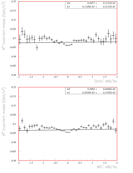
Figure 26: Invariant mass as a function of $\partial M/\partial\varepsilon$ for both data and Monte Carlo. The result of the fit is also shown. One notices that the distribution significantly departs from a straight line, however in the same way in the simulation and the data, and symmetrically around zero. Since the measurement of the curvature bias only relies on the difference between negative and positive sides of the distribution, we can measure the bias using the procedure described in the text. The systematic variations around the fit are below 1%, and we interpret them as small inaccuracies in the track model used in the track fit, which show up when averaging over a large number of tracks.

The results show that there is no momentum bias. One can give a physical interpretation of the found values. A bias of 0.1 $\rm(TeV/c)^{-1}$ corresponds to a 10 $\rm TeV/c$ particle reconstructed as a straight track (infinite momentum). The bias on the momentum measurement of a 100 $\rm GeV/c$ track is of the order of 1 % and it falls down to 0.1 % for a 10 $\rm GeV/c$ track (both values are below the intrinsic resolution of the drift chambers).

The mean momentum of secondary particles produced in neutrino interactions in the NOMAD detector is lower than 10 $\rm GeV/c$. We can consider that the momentum bias has a negligible effect on the estimation of track momenta.

9 Conclusions

The primary aim of the NOMAD experiment was to search for $\rm\nu_{\mu}\rightarrow\rm\nu_{\tau}$ oscillations, using kinematical criteria to sign the presence of the $\tau$ production and decay. This was made possible thanks to a set of large drift chambers which at the same time provided the target material for neutrino interactions and the tracker of charged particles. The technology used to produce the drift field allowed the high density of measurement points which would be difficult to achieve by conventional techniques. Furthermore, these chambers were built at a reasonable cost. The chambers ran satisfactorily during 4 years, and the NOMAD experiment was able to push by more than one order of magnitude the previous limits on $\rm\nu_{\mu}\rightarrow\rm\nu_{\tau}$ [2] and $\rm\nu_{e}\rightarrow\rm\nu_{\tau}$ [28] oscillation probability in a region of neutrino masses relevant for cosmology. The chambers played also a crucial role in several precise studies of particle production in neutrino interactions [29].

References

- [1] P.Astier et al., “Search for the Oscillation ”, CERN-SPSLC/91-21, CERN-SPSLC/91-48, CERN-SPSLC/91-53.
-
[2]
J.Altegoer et al., [NOMAD Collaboration],
Phys. Lett. B431 (1998) 219
P.Astier et al., [NOMAD Collaboration], Phys. Lett. B453 (1999) 169
P.Astier et al., [NOMAD Collaboration], Phys. Lett. B483 (2000) 387 - [3] C.H.Albright, R.E.Shrock, Phys. Lett. B84 (1979) 123
-
[4]
The magnet was previously used in the UA1 experiment.
M. Barranco-Luque et al., Nucl. Instr. and Meth. A 176 (1980) 175. - [5] J.Altegoer et al., [NOMAD Collaboration], Nucl. Instr. and Meth A404 (1998) 96
-
[6]
G.Bassompierre et al., Nucl. Instr. and Meth. A403 (1998) 363;
G.Bassompierre et al., Nucl. Instr. and Meth. A411 (1998) 63 -
[7]
D.Autiero et al., Nucl. Instr. and Meth. A373 (1996) 358;
D.Autiero et al., Nucl. Instr. and Meth. A387 (1997) 352;
D.Autiero et al., Nucl. Instr. and Meth. A411 (1998) 285 - [8] A.Peisert and F.Sauli, CERN 84-08, 13 July 1984.
- [9] G.Charpak, F.Sauli and W.Duinker, Nucl. Instr. and Meth. A108 (1973) 413
- [10] A.Breskin, G.Charpak, F.Sauli, M.Atkinson and G.Schultz, Nucl. Instr. and Meth. A124 (1975) 189
- [11] V.Uros, Ph.D. Thesis, Paris VI (1995), in French
- [12] LeCroy Corp., ”Model 1876, 96 Channels Fastbus TDC manuals”.
- [13] J.-P. Meyer, Thèse d’habilitation, Paris VII (1999), in French.
- [14] Stanford Research Systems, ” Model DG535 Digital delay/Pulse generator manuals”.
- [15] M.Vo, Ph.D. Thesis, Paris VII (1996), in French
- [16] K. Eggert et al., Nucl. Instr. and Meth. A 176 (1980) 217.
- [17] LabView User Manual for Sun (September 1994 Edition), National Instruments Corporation, Austin, TX, 1992, 1994.
- [18] K.Schahmaneche, Ph.D. Thesis, Paris VI (1997), in French
- [19] E.Gangler, Ph.D. Thesis, Paris VI (1997), in French
- [20] N.Besson, Ph.D. Thesis, DAPNIA-SPP-99-1005 (1999), in French
-
[21]
B.A.Popov, Ph.D. Thesis, Paris VII (1998)
http://www-lpnhep.in2p3.fr/Thesards/lestheses.html
http://nuweb.jinr.ru/popov - [22] P.Astier, A.Cardini, R.D.Cousins, A.Letessier-Selvon, B.A.Popov, T.Vinogradova, Nucl. Instr. and Meth. A450 (2000) 138
- [23] R.Frühwirth, Application of Filter Methods to the Reconstruction of Tracks And Vertices in Events of Experimental High Energy Physics, HEPHY-PUB 516/88 Vienna, December 1988
- [24] P.Billoir et al., Nucl. Instr. and Meth. A241 (1985) 115
- [25] P.Rathouit, Ph.D. Thesis, DAPNIA/SPHN-97-03T (1997), in French
- [26] C.Lachaud, Ph.D. Thesis, Paris VII (2000), in French
- [27] Review of Particle Properties, Eur. Phys. J. C15 (2000)
- [28] P.Astier et al., [NOMAD Collaboration], Phys. Lett. B471 (2000) 406
-
[29]
J.Altegoer et al., [NOMAD Collaboration],
Phys. Lett. B428 (1998) 197
J.Altegoer et al., [NOMAD Collaboration], Phys. Lett. B445 (1999) 439
P.Astier et al., [NOMAD Collaboration], Phys. Lett. B479 (2000) 371
P.Astier et al., [NOMAD Collaboration], Phys. Lett. B486 (2000) 35
P.Astier et al., [NOMAD Collaboration], Nucl. Phys. B588 (2000) 3
P.Astier et al., [NOMAD Collaboration], Nucl. Phys. B601 (2001) 3
P.Astier et al., [NOMAD Collaboration], Nucl. Phys. B605 (2001) 3