Abstract

This paper discusses hadron energy reconstruction for the ATLAS barrel prototype combined calorimeter (consisting of a lead-liquid argon electromagnetic part and an iron-scintillator hadronic part) in the framework of the non-parametrical method. The non-parametrical method utilizes only the known $e/h$ ratios and the electron calibration constants and does not require the determination of any parameters by a minimization technique. Thus, this technique lends itself to an easy use in a first level trigger. The reconstructed mean values of the hadron energies are within $\pm 1\%$ of the true values and the fractional energy resolution is $[(58\pm 3)\%/\sqrt{E}+(2.5\pm 0.3)\%]\oplus(1.7\pm 0.2)/E$. The value of the $e/h$ ratio obtained for the electromagnetic compartment of the combined calorimeter is $1.74\pm 0.04$ and agrees with the prediction that $e/h>1.7$ for this electromagnetic calorimeter. Results of a study of the longitudinal hadronic shower development are also presented. The data have been taken in the H8 beam line of the CERN SPS using pions of energies from 10 to 300 GeV.
Codes PACS: 29.40.Vj, 29.40.Mc, 29.85.+c.
Keywords: Calorimetry, Combined Calorimeter, Shower Counter, Compensation, Energy Measurement, Computer Data Analysis.

1 Introduction

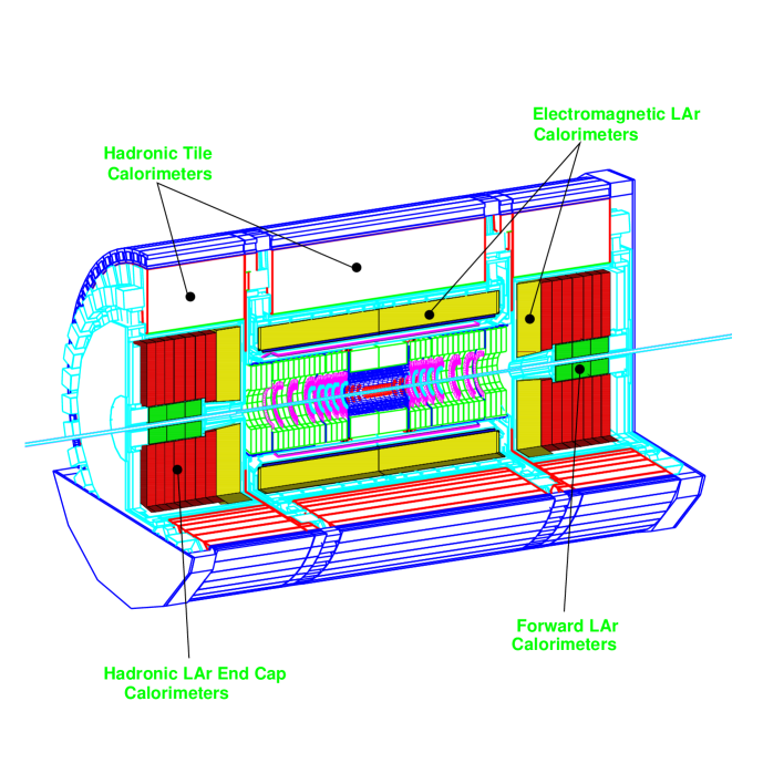
The key question for calorimetry in general, and hadronic calorimetry in particular, is that of energy reconstruction. This question becomes especially important when a hadronic calorimeter has a complex structure incorporating electromagnetic and hadronic compartments with different technologies. This is the case for the central (barrel) calorimetry of the ATLAS detector which has the electromagnetic liquid argon accordion and hadronic iron-scintillator Tile calorimeters [1, 2, 3]. A view of the ATLAS detector, including the two calorimeters, is shown in Fig. 1.

In this paper, we describe a non-parametrical method of energy reconstruction for a combined calorimeter known as the $e/h$ method, and demonstrate its performance using the test beam data from the ATLAS combined prototype calorimeter. For the energy reconstruction and description of the longitudinal development of a hadronic shower, it is necessary to know the $e/h$ ratios, the degree of non-compensation, of these calorimeters. Detailed information about the $e/h$ ratio for the ATLAS Tile barrel calorimeter is presented in [2, 4, 5, 6, 7] while much less was done so far for the liquid argon electromagnetic calorimeter [8, 9, 10]. An additional aim of the present work, then, is to also determine the value of the $e/h$ ratio for the electromagnetic compartment.

Another important question for hadron calorimetry is that relating to the longitudinal development of hadronic showers. This question is especially important for a combined calorimeter because of the different degrees of non-compensation for the separate calorimeter compartments. Information about the longitudinal hadronic shower development is very important for fast and full hadronic shower simulations and for fast energy reconstruction in a first level trigger. This work is also devoted to the study of the longitudinal hadronic shower development in the ATLAS combined calorimeter.

This work has been performed using the 1996 combined test beam data [11, 12] taken in the H8 beam line of the CERN SPS using pions of energies from 10 to 300 GeV.

2 Combined Calorimeter

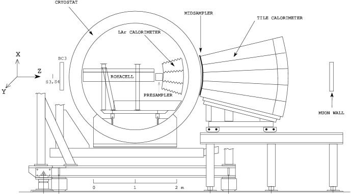
The combined calorimeter prototype setup is shown in Fig. 2, along with a definition of the coordinate system used for the test beam. The LAr calorimeter prototype is housed inside a cryostat with the hadronic Tile calorimeter prototype located downstream.

The beam line is in the $YZ$ plane at 12 degrees from the $Z$ axis. With this angle the two calorimeters have an active thickness of 10.3 interaction lengths ($\lambda_{I}$). The beam quality and geometry were monitored with a set of scintillation counters S1 – S4, beam wire chambers BC1 – BC3 and trigger hodoscopes (midsampler) placed downstream of the cryostat. To detect punchthrough particles and to measure the effect of longitudinal leakage a “muon wall” consisting of 10 scintillator counters (each 2 cm thick) was located behind the calorimeters at a distance of about 1 metre.

The liquid argon electromagnetic calorimeter prototype consists of a stack of three azimuthal modules, each module spanning $9^{\circ}$ in azimuth and extending over 2000 mm along the $Y$ direction. The calorimeter structure is defined by 2.2 mm thick steel-plated lead absorbers folded into an accordion shape and separated by 3.8 mm gaps filled with liquid argon. The signals are collected by three-layer copper-polyamide electrodes located in the gaps. The calorimeter extends from an inner radius of 1315 mm to an outer radius of 1826 mm, representing (in the $Z$ direction) a total of 25 radiation lengths ($X_{0}$), or 1.22 $\lambda_{I}$ for protons. The calorimeter is longitudinally segmented into three compartments of $9\ X_{0}$, $9\ X_{0}$ and $7\ X_{0}$, respectively. The $\eta\times\phi$ segmentation is $0.018\times 0.02$ for the first two longitudinal compartments and $0.036\times 0.02$ for the last compartment. Each read-out cell has full projective geometry in $\eta$ and $\phi$. The cryostat has a cylindrical shape, with a 2000 mm internal diameter (filled with liquid argon), and consists of an 8 mm thick inner stainless-steel vessel, isolated by 300 mm of low-density foam (Rohacell), which is itself covered by a 1.2 mm thick aluminum outer wall. A presampler was mounted in front of the electromagnetic calorimeter. The presampler has fine strips in the $\eta$ direction and covers $\thickapprox 11\times 8$ in $\eta\times\phi$ LAr calorimeter cells in the region of the beam impact. The active depth of liquid argon in the presampler was 10 mm and the strip spacing 3.9 mm. Early showers in the liquid argon were kept to a minimum by placing light foam material (Rohacell) in the cryostat upstream of the LAr electromagnetic calorimeter. The total amount of material between BC3 and LAr calorimeter is near $0.2\lambda_{I}$. More details about this prototype can be found in [1, 10].

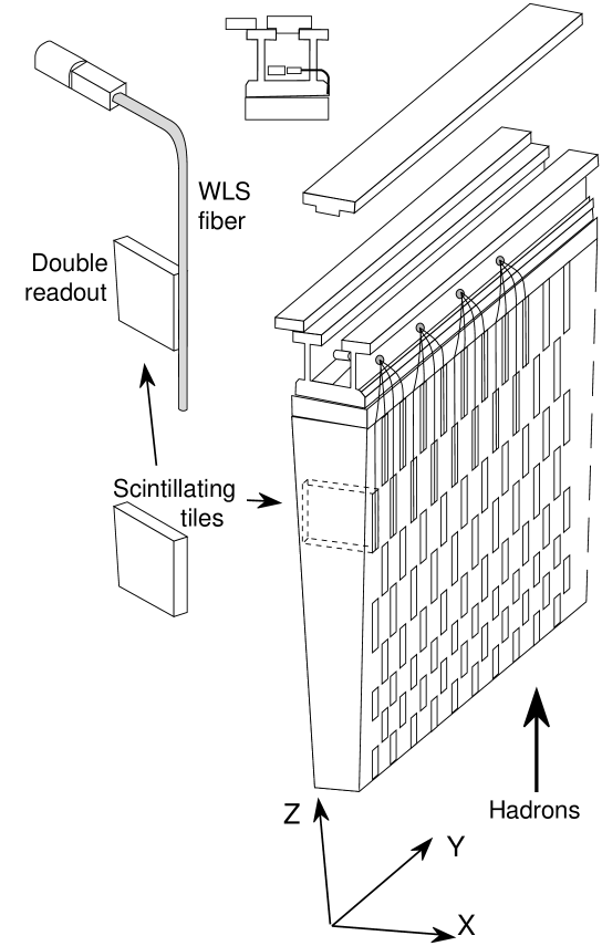
The hadronic Tile calorimeter is a sampling device which uses steel as the absorber and scintillating tiles as the active material [2]. A conceptual design of this calorimeter geometry is shown in Fig.  3. The innovative feature of the design is the orientation of the tiles which are placed in planes perpendicular to the $Y$ direction [13]. The absorber structure is a laminate of steel plates of various dimensions stacked along $Y$. The basic geometrical element of the stack is denoted as a period. A period consists of a set of two master plates (large trapezoidal steel plates, 5 mm thick, spanning along the entire $Z$ dimension) and one set of spacer plates (small trapezoidal steel plates, 4 mm thick, 100 mm wide along $Z$). During construction, the half-period elements are pre-assembled starting from an individual master plate and the corresponding 9 spacer plates. The relative position of the spacer plates in the two half periods is staggered in the $Z$ direction, to provide pockets in the structure for the subsequent insertion of the scintillating tiles. Each stack, termed a module, spans $2\pi/64$ in the azimuthal angle ($X$ dimension), 1000 mm in the $Y$ direction and 1800 mm in the $Z$ direction (about 9 $\lambda_{I}$ or about 80 $X_{0}$). The module front face, exposed to the beam particles, covers 1000$\times$200 mm². The scintillating tiles are made out of polystyrene material of thickness 3 mm, doped with scintillating and wavelength-shifting dyes. The iron to scintillator ratio is $4.67:1$ by volume. The tile calorimeter thickness along the beam direction at the incidence angle of $12^{\circ}$ (the angle between the incident particle direction and the normal to the calorimeter front face) corresponds to 1.5 m of iron equivalent length.

Wavelength shifting fibers collect the scintillation light from the tiles at both of their open (azimuthal) edges and transport it to photo-multipliers (PMTs) at the periphery of the calorimeter (Fig. 3). Each PMT views a specific group of tiles through the corresponding bundle of fibers. The prototype Tile calorimeter used for this study is composed of five modules stacked in the $X$ direction, as shown in Fig.  2.

The modules are longitudinally segmented (along $Z$) into four depth segments. The readout cells have a lateral dimension of 200 mm along $Y$, and longitudinal dimensions of 300, 400, 500, 600 mm for depth segments 1 – 4, corresponding to 1.5, 2, 2.5 and 3 $\lambda_{I}$, respectively. Along the $X$ direction, the cell sizes vary between about 200 and 370 mm depending on the $Z$ coordinate (Fig. 2). More details of this prototype can be found in [1, 14, 15, 4, 16, 17]. The energy release in 100 different cells was recorded for each event [14].

The data have been taken in the H8 beam line of the CERN SPS using pions of energy 10, 20, 40, 50, 80, 100, 150 and 300 GeV. We have applied some cuts similar to [11, 12] in order to eliminate the non-single track pion events, the beam halo, the events with an interaction before the liquid argon calorimeter, and the electron and muon events. The set of cuts adopted is as follows: single-track pion events were selected by requiring the pulse height of the beam scintillation counters and the energy released in the presampler of the electromagnetic calorimeter to be compatible with that for a single particle; the beam halo events were removed with appropriate cuts on the horizontal and vertical positions of the incoming track impact point and the space angle with respect to the beam axis as measured with the beam chambers; a cut on the total energy rejects incoming muons.

3 The $e/h$  Method of Energy Reconstruction

An hadronic shower in a calorimeter can be seen as an overlap of a pure electromagnetic and a pure hadronic component. In this case an incident hadron energy is $E=E_{e}+E_{h}$. The calorimeter response, $R$, to these two components is usually different [18, 19] and can be written as:

$$R=e\cdot E_{e}+h\cdot E_{h}\ ,$$ (1)

where $e$ ($h$) is a coefficient to rescale the electromagnetic (hadronic) energy content to the calorimeter response. A fraction of an electromagnetic energy of a hadronic shower is $f_{\pi^{0}}=E_{e}/E$, than $R=e\cdot f_{\pi^{0}}\cdot E+h\cdot(E-f_{\pi^{0}}\cdot E)=e\cdot[1+(e/h-1)\cdot f_{\pi^{0}}]/(e/h)\cdot E$. From this one can gets formulae for an incident energy

$$E=\frac{1}{e}\cdot\Biggl{(}\frac{e}{\pi}\Biggr{)}\cdot R\ ,$$ (2)

where

$$\Biggl{(}\frac{e}{\pi}\Biggr{)}=\frac{e/h}{1+(e/h-1)\cdot f_{\pi^{0}}}\ .$$ (3)

The dependence of $f_{\pi^{0}}$ from the incident hadron energy can be parameterized as in Ref. [20]:

$$f_{\pi^{0}}=k\cdot\ln{E}\ .$$ (4)

In the case of the combined setup described in this paper, the total energy is reconstructed as the sum of the energy deposit in the electromagnetic compartment ($E_{LAr}$), the deposit in the hadronic calorimeter ($E_{Tile}$), and that in the passive material between the LAr and Tile calorimeters ($E_{dm}$). Expression (2) can then be rewritten as:

$$E=E_{LAr}+E_{dm}+E_{Tile}=\frac{1}{e_{LAr}}\Biggl{(}\frac{e}{\pi}\Biggr{)}_{LAr}R_{LAr}+E_{dm}+\frac{1}{e_{Tile}}\Biggl{(}\frac{e}{\pi}\Biggr{)}_{Tile}R_{Tile}\ ,$$ (5)

where $R_{LAr}$ ($R_{Tile}$) is the measured response of the LAr (Tile) calorimeter compartment and $1/e_{Tile}$ and $1/e_{LAr}$ are energy calibration constants for the LAr and Tile calorimeters respectively [11].

Similarly to the procedure in Refs. [11, 21], the $E_{dm}$ term, which accounts for the energy loss in the dead material between the LAr and Tile calorimeters, is taken to be proportional to the geometrical mean of the energy released in the third depth of the electromagnetic compartment and the first depth of the hadronic compartment ($E_{dm}=\alpha\cdot\sqrt{E_{LAr,3}\cdot E_{Tile,1}}$). The validity of this approximation has been tested using a Monte Carlo simulation along with a study of the correlation between the energy released in the midsampler and the $E_{dm}$ [12, 22, 23].

The ratio $(e/h)_{Tile}=1.30\pm 0.03$ has been measured in a stand-alone test beam run [6] and is used to determine the $(e/\pi)_{Tile}$ term in equation 5. To determine the value of the $1/e_{Tile}$ constant we selected events which started showering only in the hadronic compartment, requiring that the energy deposited in each sampling of the LAr calorimeter and in the midsampler is compatible with that of a single minimum ionization particle. The result is $1/e_{Tile}=0.145\pm 0.002$.

The response of the LAr calorimeter has already been calibrated to the electromagnetic scale; thus the constant $1/e_{LAr}=1$ [11, 12]. The value of $(e/h)_{LAr}$ has been evaluated using the data from this beam test, selecting events with well developed hadronic showers in the electromagnetic calorimeter, i.e. events with more than 10% of the beam energy in the electromagnetic calorimeter. Using the expression (5), the $(e/\pi)_{LAr}$ ratio can be written as:

$$\Biggl{(}\frac{e}{\pi}\Biggr{)}_{LAr}=\frac{E_{beam}-E_{dm}-E_{Tile}}{R_{LAr}/e_{LAr}}\ .$$ (6)

Fig.  4 shows the distributions of the $(e/\pi)_{LAr}$ ratio for different energies, and the mean values of these distributions are plotted in Fig. 5 as a function of the beam energy. From a fit to this distribution using expression (3) and (4) we obtain $(e/h)_{LAr}=1.74\pm 0.04$ and $k=0.108\pm 0.004$, thereby taking $(e/h)_{LAr}$ to be energy independent. For a fixed value of the parameter $k=0.11$ [20], the result is $(e/h)_{LAr}=1.77\pm 0.02$. The quoted errors are the statistical ones obtained from the fit. The systematic error on the $(e/h)_{LAr}$ ratio, which is a consequence of the uncertainties in the input constants used in the equation (6) as well as of the shower development selection criteria, is estimated to be $\pm 0.04$.

Figure 6 compares our values of the $(e/\pi)_{LAr}$ ratio to the ones obtained in Refs. [8, 9, 10] using a weighting method. The results are in good agreement below 100 GeV but disagree above this energy because the weighting method leads to a distortion of the $(e/\pi)_{LAr}$ ratios. Despite this disagreement, fitting expression (3) to the old data leads to $(e/h)_{em}=1.73\pm 0.10$ for [9] and $(e/h)_{em}=1.64\pm 0.18$ for [10] (parameter $k$ fixed at 0.11). These values are in agreement with our result within error bars.

In the Ref. [20] it was demonstrated that the $e/h$ ratio for non-uranium calorimeters with high-$Z$ absorber material is satisfactorily described by the formula:

$$\frac{e}{h}=\frac{e/mip}{0.41+f_{n}\cdot n/mip}\ ,$$ (7)

where $f_{n}$ is a constant determined by the $Z$ of the absorber (for lead $f_{n}=0.12$) [24, 25], and $e/mip$ and $n/mip$ represent the calorimeter response to electromagnetic showers and to MeV-type neutrons, respectively. These responses are normalized to the one for minimum ionizing particles. The Monte Carlo calculated $e/mip$ and $n/mip$ values [18] for the lead liquid argon electromagnetic calorimeter [26] are $e/mip=0.78$ and $n/mip<0.5$, leading to $e/h>1.66$. The measured value of the $(e/h)_{em}$ ratio agrees with this prediction. Using expression (7) and measured value of $e/h$ we can find that $n/mip$ is $\simeq 0.3$.

Formula (7) indicates that $e/mip$ is very important for understanding compensation in lead liquid argon calorimeters. The degree of non-compensation increases when the sampling frequency is also increased [24]. A large fraction of the electromagnetic energy is deposited through very soft electrons ($E<1$ MeV) produced by Compton scattering or the photoelectric effect. The cross sections for these processes strongly depend on $Z$ and practically all these photon conversions occur in the absorber material. The range of the electrons produced in these processes is very short, $\sim 0.7$ mm for 1 MeV electron in lead. Such electrons only contribute to the calorimeter signal if they are produced near the boundary between the lead and the active material. If the absorber material is made thinner this effective boundary layer becomes a larger fraction of the total absorber mass and the calorimeter response goes up. This effect was predicted by EGS3 simulation [27]. It leads to predictions for the GEM [28] accordion electromagnetic calorimeter (1 mm lead and 2 mm liquid argon) that $e/mip=0.86$ and $e/h>1.83$. The Monte Carlo calculations also predict that the electromagnetic response for liquid argon calorimeters (due to the larger $Z$ value of argon) is consistently larger than for calorimeters with plastic-scintillator readout. The signal from neutrons ($n/mip$) is suppressed by a factor $0.12$ and the $n-p$ elastic scattering products do not contribute to the signal of liquid argon calorimeters. These detectors only observe the $\gamma$’s produced by inelastic neutron scattering (thermal neutron capture escapes detection because of fast signal shaping) [24].

To use expression (5) for reconstructing incident hadron energies, it is necessary to know the $(e/\pi)_{Tile}$ and $(e/\pi)_{LAr}$ ratios, which themselves depend on the hadron energy. For this purpose, a two cycle iteration procedure has been developed. In the first cycle, the $(e/\pi)_{Tile}$ ratio is iteratively evaluated using the expression:

$$\Biggl{(}\frac{e}{\pi}\Biggr{)}_{Tile}=\frac{(e/h)_{Tile}}{1+((e/h)_{Tile}-1)\cdot k\cdot\ln{(1/e_{Tile}\cdot(e/\pi)_{Tile}\cdot R_{Tile})}}\ .$$ (8)

using the value of $(e/\pi)_{Tile}$ from a previous iteration. To start this procedure, a value of 1.13 (corresponding to $f_{\pi}^{0}=0.11\ln(100$ GeV$)$) has been used.

In the second cycle, the first approximation of the energy, $E$, is calculated using the equation (5) with the $(e/\pi)_{Tile}$ ratio obtained in the first cycle and the $(e/\pi)_{LAr}$ ratio from equation (3), where again the iteration is initiated by $f_{\pi^{0}}=0.11\ln(100$ GeV$)$.

In both cycles the iterated values are arguments of a logarithmic function; thus the iteration procedure is very fast. After the first iteration, an accuracy of about $0.1\%$ has been achieved for energies in the range 80$\div$150 GeV, while a second iteration is needed to obtain the same precision for the other beam energies. In Fig. 7 the energy linearity, defined as the ratio between the mean reconstructed energy and the beam energy, is compared, after a first iteration, to the linearity obtained after iterating to a $\epsilon=0.1\%$ accuracy, showing a good agreement. For this reason, the suggested algorithm of the energy reconstruction can be used for the fast energy reconstruction in a first level trigger.

Fig. 7 also demonstrates the correctness of the mean energy reconstruction. The mean value of $E/E_{beam}$ is equal to $(99.5\pm 0.3)\%$ and the spread is $\pm 1\%$, except for the point at 10 GeV. However, as noted in [11], result at 10 GeV is strongly dependent on the effective capability to remove events with interactions in the dead material upstream and to separate the real pion contribution from the muon contamination.

Fig.  8 shows the pion energy spectra reconstructed with the $e/h$ method proposed in this paper for different beam energies. The mean and $\sigma$ values of these distributions are extracted with Gaussian fits over $\pm 2\sigma$ range and are reported in Table 1 together with the fractional energy resolution.

Fig. 9 shows the comparison of the linearity as a function of the beam energy for the $e/h$ method and for the cells weighting method [29]. Comparable quality of the linearity is observed for these two methods.

Fig. 10 shows the fractional energy resolutions ($\sigma/E$) as a function of $1/\sqrt{E}$ obtained by three methods: the $e/h$ method (black circles, also presented on the Table 1), the benchmark method [11] (crosses), and the cells weighting method [11] (open circles). The energy resolutions for the $e/h$ method are comparable with the benchmark method and only $30\%$ worse than for the cells weighting method. A fit to the data points gives the fractional energy resolution for the $e/h$ method obtained using the iteration procedure with $\epsilon=0.1\%$,

$$\sigma/E=[(58\pm 3)\%/\sqrt{E}+(2.5\pm 0.3)\%]\oplus(1.7\pm 0.2)/E$$ (9)

for the $e/h$ method using the first approximation,

$$\sigma/E=[(56\pm 3)\%/\sqrt{E}+(2.7\pm 0.3)\%]\oplus(1.8\pm 0.2)/E,$$ (10)

for the benchmark method,

$$\sigma/E=[(60\pm 3)\%/\sqrt{E}+(1.8\pm 0.2)\%]\oplus(2.0\pm 0.1)/E,$$ (11)

and, for the cells weighting method,

$$\sigma/E=[(42\pm 2)\%/\sqrt{E}+(1.8\pm 0.1)\%]\oplus(1.8\pm 0.1)/E,$$ (12)

where E is in GeV and the symbol $\oplus$ indicates a sum in quadrature. The sampling term is consistent between the $e/h$ method and the benchmark method and is smaller by a factor of 1.5 for the cells weighting method. The constant term is the same for the benchmark method and the cells weighting method and is larger by $(0.7\pm 0.3)\%$ for the $e/h$ method. The noise term of about $1.8$ GeV coincide for all four cases within errors that reflect its origin in electronic noise. Note, that from the pedestal trigger data the total noise for the two calorimeters was estimated to be about 1.4 GeV.

4 Hadronic Shower Development

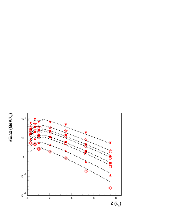
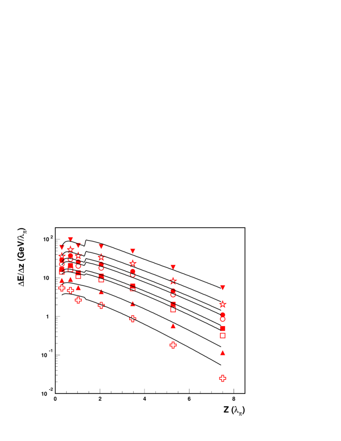
The $e/h$ method for energy reconstruction has been used to study the energy depositions, $E_{i}$, in each longitudinal calorimeter sampling. Table 2 lists (and Fig. 11 shows) the differential mean energy depositions $(\Delta E/\Delta z)_{i}=E_{i}/\Delta z_{i}$ as a function of the longitudinal coordinate $z$ for energies from 10 to 300 GeV, with $z$ expressed in interaction length units.

A well known parameterization of the longitudinal hadronic shower development from the shower origin is suggested in Ref. [30]:

$$\frac{dE_{s}(z)}{dz}=N\ \Biggl{\{}\omega\ \biggl{(}\frac{z}{X_{0}}\biggr{)}^{a-1}\ e^{-b\frac{z}{X_{0}}}\ +\ (1-\omega)\ \biggl{(}\frac{z}{\lambda_{I}}\biggr{)}^{a-1}\ e^{-d\frac{z}{\lambda_{I}}}\Biggr{\}}\ ,$$ (13)

where $N$ is the normalization factor, and $a,\ b,\ d,\ \omega$ are parameters ($a=0.6165+0.3183\cdot\ln{E}$, $b=0.2198$, $d=0.9099-0.0237\cdot\ln{E}$, $\omega=0.4634$). In this parameterization, the origin of the $z$ coordinate coincides with shower origin, while our data are from the calorimeter face and, due to insufficient longitudinal segmentation, the shower origin can not be inferred to an adequate precision. Therefore, an analytical representation of the hadronic shower longitudinal development from the calorimeter face has been used [31]:

$$\frac{dE(z)}{dz} = N\ \Biggl{\{}\frac{\omega X_{0}}{a}\biggl{(}\frac{z}{X_{0}}\biggr{)}^{a}e^{-b\frac{z}{X_{0}}}{}_{1}F_{1}\biggl{(}1,a+1,\biggl{(}b-\frac{X_{0}}{\lambda_{I}}\biggr{)}\frac{z}{X_{0}}\biggr{)}$$ (14)

$$+\ \frac{(1-\omega)\lambda_{I}}{a}\biggl{(}\frac{z}{\lambda_{I}}\biggr{)}^{a}e^{-d\frac{z}{\lambda_{I}}}{}_{1}F_{1}\biggl{(}1,a+1,\bigl{(}d-1\bigr{)}\frac{z}{\lambda_{I}}\biggr{)}\Biggr{\}},$$

where ${}_{1}F_{1}(\alpha,\beta,z)$ is the confluent hypergeometric function. Note that the formula (14) is given for a calorimeter characterized by its $X_{0}$ and $\lambda_{I}$. In the combined setup, the values of $X_{0}$, $\lambda_{I}$ and the $e/h$ ratios are different for electromagnetic and hadronic compartments. So, the use of formula (14) is not straightforward for the description of the hadronic shower longitudinal profiles.

To overcome this problem, Ref. [32] suggests an algorithm to combine the electromagnetic calorimeter ($em$) and hadronic calorimeter ($had$) curves of the differential longitudinal energy deposition $dE/dz$. At first, the mean hadronic shower develops according eq. (14) in the electromagnetic calorimeter to the boundary value $z_{em}$ which corresponds to a certain integrated measured energy $E_{em}(z_{em})$. Then, using the corresponding integrated hadronic curve, $E(z)=\int_{0}^{z}(dE/dz)dz$, the point $z_{had}$ is found from the equation $E_{had}(z_{had})=E_{em}(z_{em})+E_{dm}$. From this point a shower continues to develop in the hadronic calorimeter. In principle, instead of the measured value of $E_{em}$ one can use the calculated value of $E_{em}=\int_{0}^{z_{em}}(dE/dz)dz$ obtained from the integrated electromagnetic curve. The combined curves have been obtained in this manner.

Fig. 11 shows the differential energy depositions $(\Delta E/\Delta z)_{i}=E_{i}/\Delta z_{i}$ as a function of the longitudinal coordinate $z$ in units of $\lambda_{\pi}$ for the energy from 10 to 300 GeV and a comparison with the combined curves for the longitudinal hadronic shower profiles (dashed lines). The level of agreement was estimated using the function $\chi^{2}$ where, following Ref. [30], the variances of the energy depositions are taken to be equal to the depositions themselves. A significant disagreement ($P(\chi^{2})<0.1\%$) has been observed between the experimental data and the combined curves in the region of the LAr calorimeter, especially at low energies.

We attempted to improve the description and to include such essential feature of a calorimeter as the $e/h$ ratio. Several modifications and adjustments of some parameters of the parameterization (14) have been tried. The conclusion is that replacing the two parameters $b$ and $\omega$ in the formula (14) with $b=0.22\cdot(e/h)_{cal}/(e/h)_{cal}^{\prime}$ and $\omega=0.6\cdot(e/\pi)_{cal}/(e/\pi)_{cal}^{\prime}$ results in a reasonable description of the experimental data. Here the values of the $(e/h)_{cal}^{\prime}$ ratios are $(e/h)^{\prime}_{em}\approx 1.1$ and $(e/h)^{\prime}_{had}\approx 1.3$ which correspond to the data used for the Bock et al. parameterization [30]. The $(e/\pi)_{cal}^{\prime}$ are calculated using formulas (3) and (4).

In Fig. 12 the experimental differential longitudinal energy depositions and the results of the description by the modified parameterization (solid lines) are compared. There is a reasonable agreement (the probability of description is more than $5\%$) between the experimental data and the curves. Note, that previous comparisons between Monte-Carlo and data have shown that FLUKA describes well the longitudinal shape of hadronic showers [11].

The obtained parameterization has some additional applications. For example, this formula may be used for an estimate of the energy deposition in various parts of a combined calorimeter. This is demonstrated in Fig. 13 in which the measured and calculated relative values of the energy deposition in the LAr and Tile calorimeters are presented. The errors of the calculated values presented in this figure reflect the uncertainties of the parameterization (14). The relative energy deposition in the LAr calorimeter decreases from about 50% at 10 GeV to 30% at 300 GeV. Conversely, the fraction in the Tile calorimeter increases as the energy increases.

5 Conclusions

Hadron energy reconstruction for the ATLAS barrel prototype combined calorimeter has been carried out in the framework of the non-parametrical method. The non-parametrical method of the energy reconstruction for a combined calorimeter uses only the $e/h$ ratios and the electron calibration constants, without requiring the determination of other parameters by a minimization technique. Thus, it can be used for the fast energy reconstruction in a first level trigger. The value of the $e/h$ ratio obtained for the electromagnetic compartment of the combined calorimeter is $1.74\pm 0.04$ and agrees with the prediction that $e/h>1.66$ for this calorimeter. The ability to reconstruct the mean values of particle energies (for energies larger than 10 GeV) within $\pm 1\%$ has been demonstrated. The obtained fractional energy resolution is $[(58\pm 3)\%/\sqrt{E}+(2.5\pm 0.3)\%]\oplus(1.7\pm 0.2)/E$. The results of the study of the longitudinal hadronic shower development have also been presented.

6 Acknowledgments

We would like to thank the technical staffs of the collaborating Institutes for their important and timely contributions. Financial support is acknowledged from the funding agencies of the collaborating Institutes. Finally, we are grateful to the staff of the SPS, and in particular to Konrad Elsener, for the excellent beam conditions and assistance provided during our tests.

Table 1: Mean reconstructed energy, energy resolution and fractional energy resolution for the various beam energies.

$E_{beam}$	$E$ (GeV)	$\sigma$ (GeV)	$\sigma/E\ (\%)$
$10^{\ast}$ GeV	$9.30\pm 0.07$	$2.53\pm 0.05$	$27.20\pm 0.58$
$20^{\star}$ GeV	$19.44\pm 0.06$	$3.41\pm 0.06$	$17.54\pm 0.31$
40 GeV	$39.62\pm 0.11$	$5.06\pm 0.08$	$12.77\pm 0.21$
50 GeV	$49.85\pm 0.13$	$5.69\pm 0.13$	$11.41\pm 0.26$
80 GeV	$79.45\pm 0.16$	$7.14\pm 0.14$	$8.99\pm 0.18$
100 GeV	$99.10\pm 0.17$	$8.40\pm 0.16$	$8.48\pm 0.16$
150 GeV	$150.52\pm 0.19$	$11.20\pm 0.18$	$7.44\pm 0.12$
300 GeV	$298.23\pm 0.37$	$17.59\pm 0.33$	$5.90\pm 0.11$
∗The measured value of the beam energy is 9.81 GeV.
⋆The measured value of the beam energy is 19.8 GeV.

Table 2: The differential mean energy depositions $\Delta E/\Delta z$ ($GeV/\lambda_{\pi}$) as a function of the longitudinal coordinate $z$ for the various beam energies.

N	z	$E_{beam}$ (GeV)
depth	($\lambda_{\pi}$)	10	20	40	50
1	0.294	$5.45\pm 0.08$	$8.58\pm 0.16$	$14.3\pm 0.2$	$16.6\pm 0.4$
2	0.681	$4.70\pm 0.08$	$9.10\pm 0.15$	$16.7\pm 0.2$	$20.8\pm 0.3$
3	1.026	$2.66\pm 0.06$	$5.55\pm 0.11$	$11.1\pm 0.2$	$13.6\pm 0.2$
4	2.06	$1.93\pm 0.03$	$4.35\pm 0.06$	$8.99\pm 0.08$	$11.0\pm 0.1$
5	3.47	$0.87\pm 0.02$	$2.13\pm 0.04$	$5.29\pm 0.06$	$6.15\pm 0.10$
6	5.28	$0.18\pm 0.01$	$0.57\pm 0.02$	$1.50\pm 0.03$	$2.07\pm 0.05$
7	7.50	$0.025\pm 0.003$	$0.11\pm 0.01$	$0.32\pm 0.01$	$0.49\pm 0.02$
N	z	$E_{beam}$ (GeV)
depth	($\lambda_{\pi}$)	80	100	150	300
1	0.294	$22.6\pm 0.6$	$28.4\pm 0.6$	$36.3\pm 0.7$	$61.3\pm 1.5$
2	0.681	$30.4\pm 0.4$	$37.6\pm 0.5$	$53.5\pm 0.8$	$97.9\pm 1.7$
3	1.026	$20.3\pm 0.3$	$25.7\pm 0.4$	$37.2\pm 0.6$	$68.9\pm 1.2$
4	2.06	$18.0\pm 0.1$	$22.4\pm 0.2$	$33.9\pm 0.3$	$64.8\pm 0.7$
5	3.47	$11.9\pm 0.1$	$14.6\pm 0.2$	$23.3\pm 0.2$	$49.0\pm 0.5$
6	5.28	$3.66\pm 0.06$	$4.57\pm 0.08$	$8.18\pm 0.13$	$18.6\pm 0.3$
7	7.50	$0.86\pm 0.03$	$1.10\pm 0.04$	$2.04\pm 0.06$	$5.54\pm 0.15$

Figure 1: Three-dimensional cutaway view of the ATLAS calorimeters.

Figure 2: Schematic layout of the experimental setup for the combined LAr and Tile calorimeters run (side view). The S3 and S4 are scintillation counters, the BC3 is a beam proportional chamber, and the midsampler and the “muon wall” are scintillation hodoscopes.

Figure 3: Conceptual design of a Tile calorimeter module.

Figure 4: The distributions of the $(e/\pi)_{LAr}$ ratio for beam energies of 20 and 50 GeV (top row, left to right), and beam energies of 100 and 300 GeV (bottom row, left to right).

Figure 5: The mean value of the $(e/\pi)_{LAr}$ ratio as a function of the beam energy. The curve is the result of a fit of equations (3) and (4).

Figure 6: The $(e/\pi)_{LAr}$ ratios as a function of the beam energy. for $e/h$ method (black circles) and for weighting method (open circles for [9] and open squares for [10]). The lines are the result of a fit of equations (3) and (4) with free $e/h$ parameter and $k=0.11$: solid line is for our data, dashed line is for the [9] data and dash-doted line is for the [10] data.

Figure 7: Energy linearity as a function of the beam energy for the $e/h$ method obtained using the iteration procedure with $\epsilon=0.1\%$ (black circles) and with the first approximation (open circles).

Figure 8: The energy distributions for beam energies of 20 and 50 GeV (top row, left to right), and beam energies of 100 and 300 GeV (bottom row, left to right).

Figure 9: Energy linearity as a function of the beam energy for the $e/h$ method (black circles) and the cells weighting method (open circles).

Figure 10: The energy resolutions obtained with the $e/h$ method (black circles), the benchmark method (crosses) and the cells weighting method (circles).

Figure 11: The comparison between the experimental differential mean energy depositions at 10 GeV (crosses), 20 GeV (black top triangles), 40 GeV (open squares), 50 GeV (black squares), 80 GeV (open circles), 100 GeV (black circles), 150 GeV (stars), 300 GeV (black bottom triangles) and the calculated curves (14) as a function of the longitudinal coordinate $z$ in units $\lambda_{\pi}$. The errors on the data points are the errors of the mean values and there are within symbols size.

Figure 12: The experimental differential mean longitudinal energy depositions at 10 GeV (crosses), 20 GeV (black top triangles), 40 GeV (open squares), 50 GeV (black squares), 80 GeV (open circles), 100 GeV (black circles), 150 GeV (stars), 300 GeV (black bottom triangles) energies as a function of the longitudinal coordinate $z$ in units $\lambda_{\pi}$ for the combined calorimeter and the results of the description by the modified parameterization for the equation (14).

Figure 13: Energy deposition (percentage) in the LAr and Tile calorimeters at different beam energies. The circles (squares) are the measured energy depositions in the LAr (Tile) calorimeter, the diamonds (crosses) are the calculated energy depositions.

References

- [1] ATLAS Collaboration, ATLAS Technical Proposal for a General Purpose pp Experiment at the Large Hadron Collider, CERN/LHCC/94-93, CERN, Geneva, Switzerland.
- [2] ATLAS Collaboration, ATLAS TILE Calorimeter Technical Design Report, CERN/ LHCC/ 96-42, ATLAS TDR 3, 1996, CERN, Geneva, Switzerland.
- [3] ATLAS Collaboration, ATLAS Liquid Argon Calorimeter Technical Design Report, CERN/LHCC/96-41, ATLAS TDR 2, 1996, CERN, Geneva, Switzerland.
- [4] F. Ariztizabal et al., Construction and Performance of an Iron Scintillation Hadron Calorimeter with Longitudinal Tile Configuration, NIM A349 (1994) 384.
- [5] A. Juste, Analysis of the Hadronic Performance of the TILECAL Prototype Calorimeter and Comparison with Monte Carlo, ATL-TILECAL-95-69, 1995, CERN, Geneva, Switzerland.
- [6] J. Budagov, Y. Kulchitsky et al., Electron Response and e/h Ratio of ATLAS Iron-Scintillator Hadron Prototype Calorimeter with longitudinal Tile Configuration, JINR-E1-95-513, 1995, JINR, Dubna, Russia; ATL-TILECAL-96-72, 1996, CERN, Geneva, Switzerland.
- [7] Y. Kulchitsky et al., Non-compensation of the ATLAS barrel Tile Hadron Module-0 Calorimeter, JINR-E1-99-12, 1999, JINR, Dubna, Russia; ATL-TILECAL-99-002, 1999, CERN, Geneva, Switzerland.
- [8] M. Stipcevic, A Study of a Hadronic Liquid Argon Calorimeter Prototype for an LHC Experiment: Testing in a Beam and Optimization of Energy Resolution by Means of a Weighting Method, Thesis, LAPP-T-94-02, RD3-Note-62, 1994, LAPP, Annecy, France.
- [9] M. Stipcevic, First Evaluation of Weighting Techniques to Improve Pion Energy Resolution in Accordion Liquid Argon Calorimeter, RD3-Note-44, 18 pp., 1993, CERN, Geneva, Switzerland.
- [10] D.M. Gingrich et al., (RD3 Collaboration), Performance of a Liquid Argon Accordion Hadronic Calorimeter Prototype, CERN-PPE/94-127, 43 pp., 1994, CERN, Geneva, Switzerland; NIM A355 (1995) 290.
- [11] S. Akhmadaliev et al., (ATLAS Collaboration; Calorimetry and Data Acquisition), Results from a New Combined Test of an Electromagnetic Liquid Argon Calorimeter with a Hadronic Scintillating-Tile Calorimeter, NIM A499 (2000) 461.
- [12] M. Cobal et al., Analysis Results of the April 1996 Combined Test of the LArgon and TILECAL Barrel Calorimeter Prototypes, ATL-TILECAL-98-168, 1998, CERN, Geneva, Switzerland.
- [13] O. Gildemeister, F. Nessi-Tedaldi, M. Nessi, An Economic Concept for a Barrel Hadron Calorimeter with Iron Scintillator Sampling and Wls-fiber Readout, Proceedings: 2nd International Conference on Calorimetry in High-energy Physics, Capri, Italy, 14-18 October 1991, 199-202.
- [14] E. Berger et al., (RD34 Collaboration), Construction and Performance of an Iron-scintillator Hadron Calorimeter with Longitudinal Tile Configuration, CERN/LHCC 95-44, LRDB Status Report/RD 34, CERN, Geneva, Switzerland, 1995.
- [15] M. Bosman et al., (RD34 Collaboration), Developments for a Scintillator Tile Sampling Hadron Calorimeter with Longitudinal Tile Configuration, CERN/DRDC/93-3 (1993).
- [16] P. Amaral et al., (ATLAS Tilecal Collaboration), Hadronic Shower Development in Iron-Scintillator Tile Calorimetry, NIM A443 (2000) 51.
- [17] J. Budagov, Y. Kulchitsky et al., Study of the Hadron Shower Profiles with the ATLAS Tile Hadron Calorimeter, JINR-E1-97-318, 1997, JINR, Dubna, Russial; ATL-TILECAL-97-127, 1997, CERN, Geneva, Switzerland.
- [18] R. Wigmans, High Resolution Hadronic Calorimetry, NIM A265 (1988) 273.
- [19] D. Groom, Radiation Levels in SSC Calorimetry, SSC-229, Proceedings: Workshop on Calorimetry for the Superconducting Supercollider, Tuscaloosa, Alabama, USA (1989) 77-90.
- [20] R. Wigmans, Performance and Limitations of Hadron Calorimeters, Proceedings: 2nd International Conference on Calorimetry in High-energy Physics, Capri, Italy, 14-18 October 1991.
- [21] Z. Ajaltouni et al., (ATLAS Collaboration; Calorimetry and Data Acquisition), Results from a Combined Test of an Electromagnetic Liquid Argon Calorimeter with a Hadronic Scintillating Tile Calorimeter, NIM A387 (1997) 333.
- [22] M. Bosman, Y. Kulchitsky, M. Nessi, Charged Pion Energy Reconstruction in the ATLAS Barrel Calorimeter, JINR-E1-2000-31, 2000, JINR, Dubna, Russia; ATL-TILECAL-2000-002, 2000, CERN, Geneva, Switzerland.
- [23] ATLAS Collaboration, ATLAS Physical Technical Design Report, v.1, CERN-LHCC-99-02, ATLAS-TDR-14, CERN, Geneva, Switzerland
- [24] R. Wigmans, On the Energy resolution of Uranium and other Hadronic Calorimeters, CERN-EP/86-141, 108pp., 1986, CERN, Geneva, Switzerland, NIM A259 (1987) 389.
- [25] R. Wigmans, On the Role of Neutrons in Hadron Calorimetry, Rev. Sci. Inst., 1998, v. 69, 11, pp. 3723-3736.
- [26] G. Costa, (for the RD3 Collaboration), Liquid Argon Calorimetry with an Accordion Geometry for the LHC, Proc. 2nd Int. Conf. on Calorimetry in HEP, 237-244, Capri, Italy, 1991.
- [27] W. Flauger, Simulation of the Transition Effect in Liquid Argon Calorimeter, NIM A241 (1985) 72.
- [28] B.C. Barish, The GEM Experiment at the SSC, CALT-68-1826, Proceedings: High Energy Physics, vol.2, 1992, p.1829, Dallas, USA.
- [29] M.P. Casado, M. Cavalli-Sforza, H1-inspired Analysis of the 1994 Combined Test of the Liquid Argon and Tilecal Calorimeter Prototypes, ATL-TILECAL-96-75, 1996, CERN, Geneva, Switzerland.
- [30] R. Bock et al., Parametrization of the Longitudinal Development of Hadronic Showers in Sampling Calorimeters, NIM 186 (1981) 533.
- [31] Y. Kulchitsky, V. Vinogradov, Analytical Representation of the Longitudinal Hadronic Shower Development, NIM A413 (1998) 484.
- [32] Y. Kulchitsky, V. Vinogradov, On the Parameterization of Longitudinal Hadronic Shower Profiles in Combined Calorimetry, NIM A455 (2000) 449.